Spatially Dependent Bayesian Modeling of Geostatistics Data and Its Application for Tuberculosis (TB) in China

Abstract

Geostatistics data in regions always have highly spatial heterogeneous, yet the regional features of the data itself cannot be ignored. In this paper, a novel latent Bayesian spatial model is proposed, which incorporates the spatial dependence of different subjects and the spatial random effects to further analysis the influence of spatial effect. The model is verified to be compatible with the integrated nested Laplace approximation (INLA) framework and is fitted using INLA and stochastic partial differential equation (SPDE). The posterior marginal distribution of parameters is estimated with high precision. Additionally, a practical application of the model is presented using tuberculosis (TB) incidence data in China from 2015 to 2019. The results show that the fitting accuracy of our model is higher than the general Bayesian spatial model using INLA-SPDE.

1. Introduction

Since the 1950s, Bayesian inference has been widely applied and can be observed in almost every field. In the Bayesian framework, the posterior distribution $\pi \left(\left.\theta \right|y\right)$ of the model given parameters $\theta$ and data y is of interest. The Markov Chain Monte Carlo (MCMC [1]) algorithm is able to compute this posterior distribution effectively, but when dealing with large sample data or complex models, it encounters problems of long computation time and slow convergence. To address these problems, Rue et al. (2009) [2] proposed a new algorithm to combine Laplace approximation with modern numerical integration in the Bayesian framework, INLA. INLA can significantly conquer the problem of the high computational cost of the MCMC algorithm while ensuring fitting accuracy. Although many existing methods can approximate the marginal likelihood [3,4,5,6], INLA still has the advantages of high estimation accuracy, high computational speed, and high computational power, and its ability of parallel computation is especially important for spatial or spatio-temporal latent Gaussian models, while smaller models also enjoy good speedup.

In addition, the INLA algorithm assumes that the geostatistics data are continuous hidden Mat$\acute{\mathrm{e}}$rn Gaussian fields (GF) of a single realization. The second-order smooth isotropic Mat$\acute{\mathrm{e}}$rn GF is a solution of a SPDE [7] with Mat$\acute{\mathrm{e}}$rn covariance function (Mat$\acute{\mathrm{e}}$rn, (1960) [8]). This covariance is affected by the separation distance between spatial points, so the solution of SPDE can reflect the autocorrelation within spatial points to some extent. SPDE establishes a connection between the continuous Gaussian random field (GRF) and the discrete Gaussian Markov random field (GMRF [9]), since the precision matrix of GMRF is sparse, it allows a fast Bayesian inference. So, the INLA algorithm can be combined with SPDE. INLA-SPDE has been widely applied in various fields, including air pollution (Cameletti et al. (2013) [10]), infectious diseases (Moraga et al. (2021) [11]), species (Moraga, (2021) [12]), wildfires (Zhang et al. (2023) [13]), earthquakes (Wilson et al. (2020) [14]), etc. Detailed application of INLA-SPDE in the R-INLA software can be found in Lindgren et al. (2015) [15], Krainski et al. (2018) [16].

However, most current studies employing INLA-SPDE for spatial effects primarily focus on spatial heterogeneity or the correlation within spatial points, which is not sufficient. The spatial dependence between different subjects is also an important aspect to be considered. Anselin (1988) [17] initially introduced the concept of spatial econometrics, integrating the effects of region, location and spatially related effects into the model. Subsequently, LeSage and Pace (2009) [18] provided an overview and the application of spatial econometric models. For Bayesian inference, they utilized the MCMC algorithm to estimate the posterior distribution of the model parameters. However, although this technique provides a feasible Bayesian model-fitting method, it still has the problem of heavy computation. Bivand et al. (2014 [19], 2015 [20]) described how to use the INLA and Bayesian Model Average (BMA [21]) to fit some spatial econometrics models. Their focus was on the specification of the response and error terms commonly used in econometric models, but these models could not be directly implemented in the software at that time. Thus, they fitted several conditional models by R-INLA and then combined these models with BMA to fit spatial econometric models. In a later study, G’omez-Rubio et al. (2019) [22] proposed different methods for applying INLA to fit spatial econometric models and perform multivariate inference on the posterior. In the literature of G’omez-Rubio et al. (2020) [23], the authors utilized the INLA-BMA algorithm to fit spatial econometric models. Jiaqi Teng (2021) [24] applied the MCMCINLA method to fit a spatial lag model in a spatial econometric model. G’omez-Rubio et al. (2021) [25] described a novel class of latent models in order to fit a diverse array of spatial econometric models using R-INLA.

Based on the latent model proposed by G’omez-Rubio et al. (2021) [25], this paper proposes a new latent Bayesian spatial model under INLA-SPDE, which incorporates the spatial dependence of different subjects and the spatial random effects, thus more comprehensively accounting for the influence of spatial effects on the geostatistics data. In order to analyze the application scenarios and limitations of our proposed model, we simulate the model under the conditions of large samples, small samples and different spatial autocorrelation parameters. It is found that our proposed model has more accurate parameter estimation with large samples and strong spatial autocorrelation effects. Then, the tuberculosis (TB) incidence data in China are used as empirical data to further illustrate the effectiveness of this model. The results show that the estimation of the fixed-effects parameters remains highly accurate, and the significance of some of the fixed effects changed after accounting for spatial dependence. Therefore, this latent model can provide some references for the application of some problems in geostatistics in the future.

The structure of this paper is as follows. Section 2 presents the background of our proposed model and its construction; Section 3 offers a proof of principle demonstrating that our model can be applied under the INLA framework; Section 4 conducts numerical simulations of the proposed model to verify its correctness, giving the applicability and limitations of the proposed model; Section 5 presents the source of the TB incidence data in China and the pre-processing process of the data, giving the process of implementation and empirical analysis of INLA-SPDE based on this data; finally, Section 6 summarizes and discusses the entire paper.

2. Model Description

2.1. Background

In this section, we summarize the background and rationale for the construction of the model proposed in this paper. On the one side, in order to consider the effect of the correlation within spatial points on the response variable, there is a Bayesian spatial model with the addition of spatial random effects [7]:

$$y=X\beta +S\left(l\right)+e,$$

(1)

where $y=(y_1,y_2,\dots ,y_n)$ denotes a response variable of n regions, X is the design matrix, $\beta$ is the vector of covariate coefficients, $S\left(l\right)$ at location $l=(u,v)$ is the exact and stable solution of the SPDE, obeying a Gaussian process with zero mean, $(u,v)$ denotes the latitude and longitude coordinates of the location, e is a vector of zero mean measurement error with variance ${\sigma }_e^2$.

On the other side, in order to consider the spatial dependence of different subjects, the spatial lag model (SLM) is gaining attention from many scholars. The main model [25] is as follows:

$$y={\rho }_{lag}Wy+X\beta +e,e\sim MVN(0,{\sigma }_e^2{I}_n),$$

(2)

where ${\rho }_{lag}$ is the spatial autocorrelation, W is $n\times n$ spatial adjacency matrix. The error term e obeys the independent Gaussian distribution with mean 0, precision matrix $\tau I_n$, $\tau =1/{\sigma }_e^2$ is the precision parameter. The SLM model can be rewritten as:

$$y={(I_n-{\rho }_{lag}W)}^{-1}(X\beta +e),e\sim MVN(0,{\sigma }_e^2{I}_n).$$

(3)

In the INLA framework, SLM cannot be fitted directly, so we need to construct a latent class to refine SLM and express it as a GMRF with a sparse precision matrix to confirm the INLA framework. The latent class is:

$$x={(I_n-\rho W)}^{-1}(X\beta +e),$$

(4)

where x denotes a vector of n random effects.

For a Gaussian response, using the latent class (4), we then have the SLM latent model

$$y=x+\epsilon ,$$

(5)

where x is included as a random effect in the linear predictor and $\epsilon$ is a small error used to fit the model. The error term is only present in a Gaussian distribution and will not appear in others.

2.2. Model Construction

Considering that there is not only spatial heterogeneity but also spatial dependence in a region, this paper proposes a new latent Bayesian spatial model to analyze the influence of the spatial dependence between different subjects and the spatial heterogeneity on response variables in more detail.

In contrast with Basile et al. (2014) [26], in order to apply the model under INLA-SPDE, we add the spatial random effects to the latent model (5), which are considered to be independent of the covariates and are only used to capture the spatial heterogeneity of the spillover. The model is as follows:

$$y=x+S\left(l\right)+\epsilon ={(I_n-\rho W)}^{-1}(X\beta +e)+S\left(l\right)+\epsilon ,$$

(6)

where y denotes a response variable of length n, x is the latent spatial dependence effect, $S\left(l\right)$ denotes the spatial random effects, and $\epsilon$ is a tiny error obeying a Gaussian white noise process. The Mat$\acute{\mathrm{e}}$rn covariance function for $S\left(l\right)$ [27] is:

$$cov(S\left(l_i\right),S\left(l_j\right))={\displaystyle \frac{{\sigma }^2}{\Gamma \left(\lambda \right)2^{\lambda -1}}}{\left(\kappa ∥l_i-l_j∥\right)}^{\lambda }{K}_{\lambda }\left(\kappa ∥l_i-l_j∥\right),$$

(7)

where $∥l_i-l_j∥$ denotes the Euclidean distance between different locations, ${\sigma }^2$ is the marginal variance of the Gaussian process, $K_{\lambda }$ is a type II Bessel function, and the order $\lambda >0$ is used to measure the smoothness of the process and generally held constant. The scale parameter $\kappa$ is related to the distance range r, i.e., $r=\sqrt{8\lambda }/\kappa$ (corresponding to $\lambda >1/2$ and a distance that spatial points autocorrelation is close to 0.1).

3. Proof of GMRF Structure

In order to use INLA-SPDE to fit model (6), it is essential that the model conforms to the INLA framework, particularly to exhibit the GMRF structure with a sparse precision matrix. Therefore, this section provides a demonstration of the GMRF structure within our proposed model.

Before the proof, we split the main model (6) into two pieces, $x={(I_n-\rho W)}^{-1}(X\beta +e)$ and $S\left(l\right)$, respectively, to simplify the subsequent proof process. For the first block, assume that $\beta$ has a Gaussian prior with precision matrix Q and zero mean, i.e., $prec\left(\beta \right)=Q$ and $E\left(\beta \right)=0$. According to Bayes’ theorem, the joint distribution of x and $\beta$ for the INLA demand can be obtained as follows:

$$\pi (x,\beta )=\pi \left(x\right|\beta \left)\pi \right(\beta ).$$

Next, from the definition, assuming that the joint distribution is Gaussian and therefore the conditional distribution is also Gaussian, with

$$E\left(x\right|\beta )={\left(I_n-\rho W\right)}^{-1}X\beta ,$$

$$\begin{array}{cc}\hfill Var(x\mid \beta )& =Var\left[{\left(I_n-\rho W\right)}^{-1}X\beta +{\left(I_n-\rho W\right)}^{-1}e\mid \beta \right]\hfill \\ & ={\left(I_n-\rho W\right)}^{-1}Var(e\mid \beta ){\left({\left(I_n-\rho W\right)}^{-1}\right)}^{\prime }\hfill \\ & ={\left(I_n-\rho W\right)}^{-1}(1/prec(e\mid \beta )){\left({\left(I_n-\rho W\right)}^{-1}\right)}^{\prime }\hfill \\ & ={\left(I_n-\rho W\right)}^{-1}\frac{1}{\tau }{\left({\left(I_n-\rho W\right)}^{-1}\right)}^{\prime },\hfill \end{array}$$

$$prec(x\mid \beta )=1/Var(x\mid \beta )=\left(I_n-\rho W^{\prime }\right)\tau \left(I_n-\rho W\right).$$

The precision matrix $prec(x\mid \beta )$ is symmetric and sparse. Thus, the joint distribution of x and $\beta$ is

$$\begin{array}{cc}\hfill \pi (x,\beta )& =\pi \left(x\right|\beta \left)\pi \right(\beta )\hfill \\ & \propto exp\left\{-{\displaystyle \frac{1}{2}}{(x-E\left(x\right|\beta ))}^{{}^{\prime }}prec(x\mid \beta )(x-E\left(x\right|\beta ))\right\}exp\left\{-{\displaystyle \frac{1}{2}}{\beta }^{{}^{\prime }}Q\beta \right\}\hfill \\ & =exp\left\{-{\displaystyle \frac{1}{2}}{(x,\beta )}^{{}^{\prime }}prec(x,\beta )(x,\beta )\right\},\hfill \end{array}$$

where $prec(x,\beta )$ is the precision matrix of $(x,\beta )$ given the hyperparameters $\tau$ and $\rho$,

$$E(x,\beta )=0$$

$$prec(x,\beta )=\left(\begin{array}{cc}\tau (I_n-\rho W^{{}^{\prime }})(I_n-\rho W)& -\tau (I_n-\rho W^{{}^{\prime }})X\\ -X^{{}^{\prime }}\tau (I_n-\rho W)& Q+\tau X^{{}^{\prime }}X\end{array}\right).$$

This shows that $(x,\beta )$ obeys a normal distribution with zero mean and precision matrix $prec(x,\beta )$, so the first block has a GMRF structure. Then, due to the strongly sparse and symmetric structure of $prec(x,\beta )$, this block is allowed to use INLA for fast computation on GMRF. Details can be found in Rue et al. (2005) [9].

For the spatial random effect $S\left(l\right)$, it is the exact and stable solution of linear fractional SPDE

$${\left({\kappa }^2-\mathsf{\Delta }\right)}^{\alpha /2}\left(\omega S\left(l\right)\right)=W\left(l\right),$$

(8)

where $\mathsf{\Delta }$ is the Laplace operator, $\alpha$ controls the smoothness, $\omega$ controls the variance, and $\kappa >0$ is the scaling parameter. $S\left(l\right)$ can also be expressed using the finite element method by means of a basis function on a triangular profile defined over a domain

$$S\left(l\right)=\sum _{g=1}^G{\phi }_g\left(l\right)\widetilde{S_g}.$$

(9)

Here G is the number of vertices of the triangular profile and ${\phi }_g$ is a set of deterministic basis functions that are locally supported and segmentally linear in the triangular profile. $\widetilde{S_g}$ obeys a normal distribution with mean 0, whose value is 1 at vertex g and 0 at the other vertices. By using Neumann boundary conditions, the precision matrix Q of the normal weight vector $\tilde{S}={\tilde{S}}_1\dots {\tilde{S}}_G$ is obtained when $\alpha =2$.

$$Q={\omega }^2({\kappa }^{4}C+2{\kappa }^{2}G+G{C}^{-1}G).$$

(10)

The element of the diagonal matrix C and the sparse matrix G is $C_{ii}=\int {\phi }_i\left(l\right)dl$ and $G_{ij}=\int \nabla {\phi }_i\left(l\right)\nabla {\phi }_j\left(l\right)dl$ (∇ denotes the gradient). Since the elements of the precision matrix Q depend on $\omega$ and $\kappa$, it is a sparse matrix and $S\left(l\right)$ is a GMRF with distribution $N(0,Q^{-1})$, which meets the requirements of the INLA algorithm. Details can be found in Lindgren et al. (2011) [7].

In summary, all these components of the main model exhibit a GMRF structure with a sparse precision matrix and satisfy the criteria of the INLA algorithm.

4. Simulation Study

4.1. Data Generation

Assuming that $(I_n-\rho W)$ is reversible, we consider the general Bayesian spatial model and the Bayesian spatial model with spatial dependence and spatial random effect under INLA-SPDE in the Gaussian distribution numerically as follows:

$$y_1=x_1{\beta }_1+x_2{\beta }_2+e+S\left(l\right),$$

(11)

$$y_2={(I_n-\rho W)}^{-1}(x_1{\beta }_1+x_2{\beta }_2+e)+S\left(l\right)+\epsilon ,$$

(12)

where $y_i,i=1,2$ is the response variable, $x_1$ and $x_2$ are covariates, and ${\beta }_1$ and ${\beta }_2$ are the coefficients corresponding to the covariates. $I_n$ is the $n\times n$ unit matrix, W is the $n\ast n$ spatial weight matrix, e is the error term with $e\sim N(0,{\sigma }_e^2)$, and $\epsilon$ is a Gaussian white noise process.

The specific simulation data are taken as follows:

First, for the spatial locations coordinates $(u,v)$, we simulate it within a square domain, bounced by points $(0,0)$ in the lower left corner and $(1,1)$ in the upper right corners. Subsequently, $n=300$ locations within this domain are generated using the code $sample(1:n/n)$. Then, we can define the mesh in the given domain.

Second, in order to simulate the value of the spatial random effect $S\left(l\right)$, we set the marginal variance ${\sigma }_0^2=1$, the separation distance $r_0=0.3$ with prior $log\left(\sigma \right)=log\left({\sigma }_0\right)+{\theta }_1$ and $log\left(r\right)=log\left(r_0\right)+{\theta }_2$. Then, the prior of parameter $\kappa$ and $\omega$ can be calculated with $log\left(\kappa \right)=log\left({\kappa }_0\right)-{\theta }_2$ and $log\left(\omega \right)=log\left({\omega }_0\right)-{\theta }_1+{\theta }_2$. Here, $log\left({\sigma }_0\right)$, $log\left(r_0\right)$, $log\left({\kappa }_0\right)$, and $log\left({\omega }_0\right)$ are the baseline values. For the prior of ${\theta }_1$ and ${\theta }_2$, they are set to follow the zero-mean vague-normal independent distribution with a precision of $0.1$. Using these parameters, the precision matrix Q of SPDE can be calculated, and a sample of spatial random effects $S\left(l\right)$ is generated from GMRF using the $inla.qsample$ function.

Finally, the remaining data in the main model are simulated as follows: covariates $x_1\sim N(0,1)$, $x_2\sim N(0,1)$, parameters ${\beta }_1=3$, ${\beta }_2=5$ and ${\sigma }_e^2=0.1$. According to the coordinate points set the minimum nearest neighbor number $k=10$ by the K-Nearest Neighbor algorithm [28] to generate the weight matrix W. The model is simulated separately with $\rho =\pm 0.1,\pm 0.5,\pm 0.9$ and sample sizes of 30 and 300, respectively, under the same data seed.

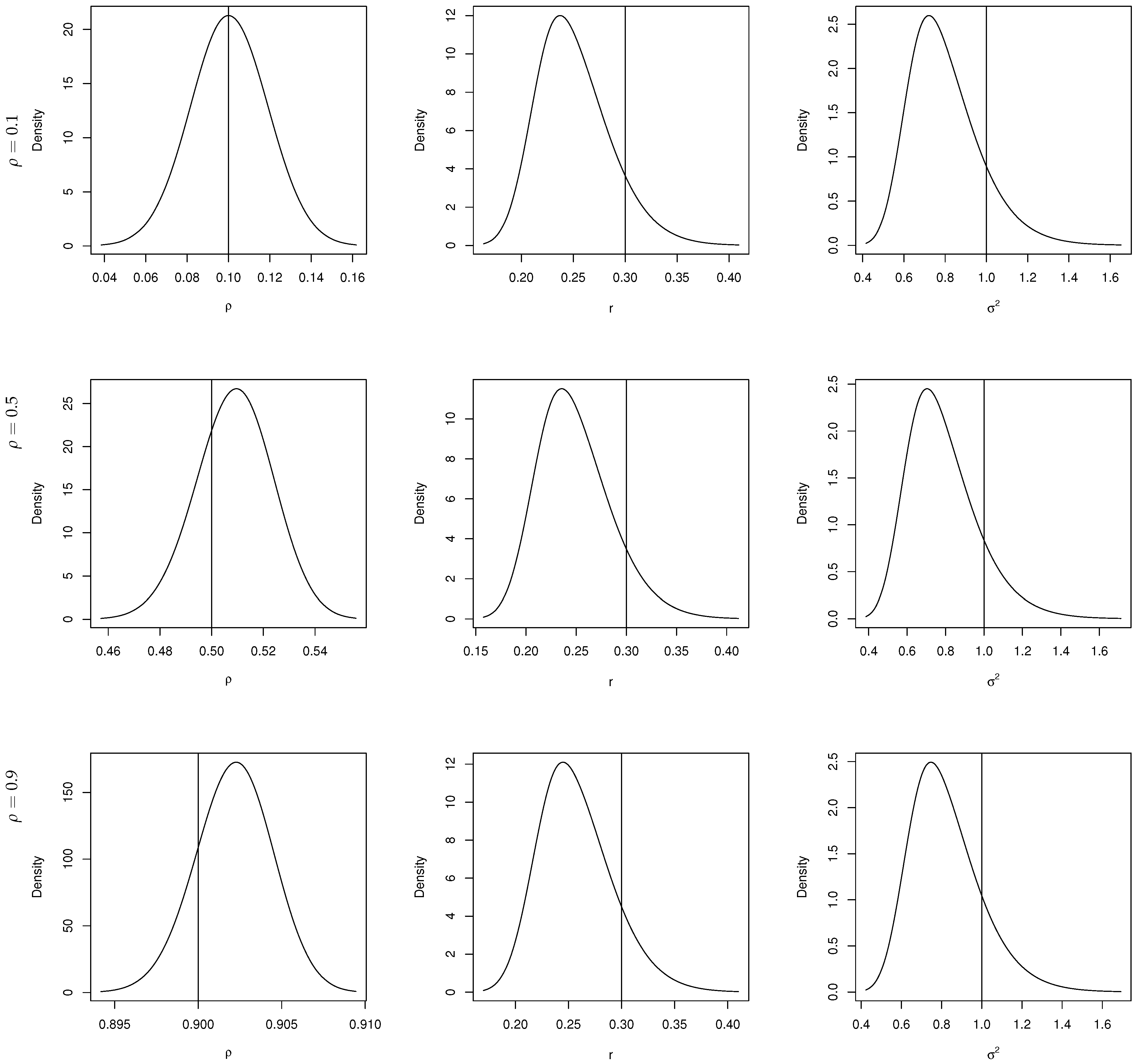
4.2. Simulation Result

Using INLA-SPDE to fit model (11) and (12) under different arithmetic cases separately, the results of the simulations are shown in

Table 1. Parameter estimation results in model (11)’s simulation.

n	$\widehat{{\mathit{\beta }}_1}$	$\widehat{{\mathit{\beta }}_2}$	r	${\mathit{\sigma }}^2$
30	3.2183 (2.9396, 3.4864)	5.0233 (4.8207, 5.2440)	0.4674 (0.2174, 0.7750)	1.5645 (0.5607, 2.8764)
300	3.0095 (2.9851, 3.0326)	5.0157 (4.9936, 5.0373)	0.2430 (0.1812, 0.3116)	0.7739 (0.4879, 1.1050)

,

Table 2. The fixed parameter estimation results in model (12)’s simulation.

n	$\mathit{\rho }$	$\widehat{\mathit{\rho }}$	r	${\mathit{\sigma }}^2$
30	−0.9	−0.8972 (−1.1348, −0.6604)	0.5180 (0.2153, 0.9279)	1.6117 (0.5110, 3.1908)
	−0.5	−0.4866 (−0.7331, −0.2472)	0.5275 (0.1578, 1.0433)	1.5465 (0.4604, 3.0258)
	−0.1	−0.0898 (−0.3238, 0.1326)	0.4904 (0.2254, 0.8168)	1.5305 (0.5246, 2.8692)
	0.1	0.1041 (−0.1156, 0.3052)	0.5035 (0.2324, 0.8561)	1.5775 (0.5622, 2.9340)
	0.5	0.5695 (0.2080, 1.0405)	0.5524 (0.1977, 0.9976)	1.5628 (0.3258, 3.4612)
	0.9	0.9009 (0.8906, 0.9116)	0.5692 (0.2339, 0.9661)	1.6231 (0.5154, 3.1612)
300	−0.9	−0.9012 (−0.9320, −0.8700)	0.2412 (0.1699, 0.3288)	0.7366 (0.4445, 1.1038)
	−0.5	−0.5013 (−0.5372, −0.4661)	0.2200 (0.1745, 0.2687)	0.6624 (0.4725, 0.8729)
	−0.1	−0.1011 (−0.1386, −0.0641)	0.2509 (0.1872, 0.3231)	0.7952 (0.4979, 1.1445)
	0.1	0.1004 (0.0638, 0.1369)	0.2508 (0.1868, 0.3230)	0.7987 (0.4999, 1.1492)
	0.5	0.5087 (0.4788, 0.5372)	0.2486 (0.1820, 0.3232)	0.7869 (0.4697, 1.1598)
	0.9	0.9021 (0.8975, 0.9065)	0.2573 (0.1938, 0.3281)	0.8233 (0.5124, 1.1841)

and

Table 3. The covariate effects coefficient estimation results in model (12)’s simulation.

n	$\mathit{\rho }$	$\widehat{{\mathit{\beta }}_1}$	$\widehat{{\mathit{\beta }}_2}$
30	−0.9	3.1819 (2.9021, 3.4626)	5.0792 (4.8317, 5.3333)
	−0.5	3.1970 (2.9155, 3.4783)	5.0607 (4.8181, 5.3127)
	−0.1	3.2031 (2.9185, 3.4852)	5.0454 (4.8073, 5.2903)
	0.1	3.1963 (2.8958, 3.4909)	5.0657 (4.8071, 5.3361)
	0.5	3.1805 (2.8550, 3.4989)	5.1152 (4.8340, 5.4198)
	0.9	3.1595 (2.8432, 3.4702)	5.1337 (4.8548, 5.4265)
300	−0.9	3.0031 (2.9762, 3.0296)	5.0096 (4.9759, 5.0436)
	−0.5	3.0049 (2.9784, 3.0307)	5.0109 (4.9791, 5.0427)
	−0.1	3.0057 (2.9786, 3.0319)	5.0128 (4.9799, 5.0458)
	0.1	3.0068 (2.9800, 3.0325)	5.0147 (4.9829, 5.0465)
	0.5	3.0084 (2.9819, 3.0339)	5.0205 (4.9919, 5.0486)
	0.9	3.0071 (2.9810, 3.0317)	5.0176 (4.9936, 5.0410)

.

According to the parameter estimation results in these tables, we can find that the models (11) and (12) fit better in the large sample case and fit with a slight error in the small sample case. In the small samples of model (12), where spatial autocorrelation is weak, the estimates of the spatial autocorrelation parameter even appear to be insignificant, this is not a positive result. These results may be because the INLA-SPDE algorithm was designed to solve the ‘big n’ problem, so we think the proposed model is more suitable for solving the large sample problem. By comparing the simulation results of these two models with large samples, it can be found that, as the spatial autocorrelation increases, more information can be captured, and the estimation of the separation distance r and marginal variance ${\sigma }^2$ between observations in the spatial random effect by model (12) is also closer to the set value compared with model (11). In summary, our model has accurate parameter estimates for autoregressive effects of varying strengths in the large sample case, with higher precision especially when spatial correlation is strong.

The fit of model (12) to the autocorrelation parameter $\rho$, separation distance r, and marginal variance ${\sigma }^2$ for a large sample with different positive spatial autocorrelation parameters is presented as a demonstration in Figure 1. The black solid curve is the fitted value of the parameter and the black solid line perpendicular to the x-axis is the setting value of the parameter.

4.3. Fitting Effect Evaluation

In this section, we test and compare different models for the model (11) with a large sample of n = 300 and model (12) with different autocorrelation parameters. The Mean Square Error (MSE) [29], the Deviant Information Criterion (DIC) [30,31], the Widely Applicable Information Xriterion (WAIC) [32,33] and the sum of the log of Conditional Predictive Ordinates (CPO) [34] values are used as model evaluation indicators to test the effect of model parameter estimation and model fitting accuracy. Here, we use ${\mathrm{CPO}}_m$ to represent the sum of the log of CPO. MSE can reflect the difference between the estimation of parameters and its true value; the smaller the value of MSE, the higher the accuracy of the estimation of parameters. The DIC, WAIC and the summary of CPO values can indicate the accuracy of model fitting; the smaller the value of DIC and WAIC, and the higher the value of ${\mathrm{CPO}}_m$, the better the model fit. However, it should be noted that when fitting model (12), we set the variance of Gaussian likelihood to a fixed tiny value by setting the log accuracy to 15, because this error term will not appear in the fitting of SLM, but this setting will cause the value of DIC, WAIC and CPO to remain unchanged no matter how the spatial autocorrelation effect changes. The results are shown in

Table 4. Comparison of model (11)’s and (12)’s simulation effect.

Model	$\mathit{\rho }$	${\mathbf{MSE}}_{{\mathit{y}}_{\mathit{i}}}$	${\mathbf{MSE}}_{{\mathit{\beta }}_1}$	${\mathbf{MSE}}_{{\mathit{\beta }}_2}$	${\mathbf{MSE}}_{\mathit{\rho }}$	${\mathbf{MSE}}_{\mathit{r}}$	${\mathbf{MSE}}_{{\mathit{\sigma }}^2}$	DIC	WAIC	CPOm
Model (11)	∖	$6.92\times {10}^{-3}$	$9.23\times {10}^{-5}$	$2.50\times {10}^{-4}$	∖	$4.35\times {10}^{-3}$	$7.60\times {10}^{-2}$	−461.15	−521.87	−11.67
Model (12)	−0.9	$1.32\times {10}^{-12}$	$9.92\times {10}^{-6}$	$9.36\times {10}^{-5}$	$2.52\times {10}^{-4}$	$5.31\times {10}^{-3}$	$1.02\times {10}^{-1}$	−3348.64	−3440.69	1450.59
	−0.5	$1.58\times {10}^{-12}$	$2.49\times {10}^{-5}$	$1.18\times {10}^{-4}$	$3.31\times {10}^{-4}$	$6.99\times {10}^{-3}$	$1.25\times {10}^{-1}$
	−0.1	$1.76\times {10}^{-12}$	$3.29\times {10}^{-5}$	$1.66\times {10}^{-4}$	$3.64\times {10}^{-4}$	$3.67\times {10}^{-3}$	$7.08\times {10}^{-2}$
	0.1	$1.87\times {10}^{-12}$	$4.67\times {10}^{-5}$	$2.18\times {10}^{-4}$	$3.48\times {10}^{-4}$	$3.69\times {10}^{-3}$	$7.05\times {10}^{-2}$
	0.5	$1.98\times {10}^{-12}$	$7.15\times {10}^{-5}$	$4.21\times {10}^{-4}$	$2.98\times {10}^{-4}$	$4.01\times {10}^{-3}$	$7.95\times {10}^{-2}$
	0.9	$2.29\times {10}^{-12}$	$5.05\times {10}^{-5}$	$3.11\times {10}^{-4}$	$9.90\times {10}^{-6}$	$3.06\times {10}^{-3}$	$6.31\times {10}^{-2}$

.

It can be visually seen that the MSE values of the response variable $y_i,i=1,2$ and the other parameters in the new latent model are very small for different settings, and the same findings are true for DIC and WAIC. Similarly, model (12) has a higher value of ${\mathrm{CPO}}_m$ than model (11). According to these results, we can conclude that the model proposed in this paper fits well under the INLA-SPDE algorithm. The conclusion further strengthens the restrictive conditions for model adaptation given in Section 4.2.

5. Empirical Analysis of Tuberculosis Incidence Data

5.1. Data Sources and Pre-Processing

Tuberculosis (TB) is an infectious disease that threatens the safety of human beings and places a great burden on people’s lives. Mainland China is a region with a high incidence of TB, and even now, with advances in medical care, there is still a need to strengthen the prevention and control of the incidence and spread of tuberculosis.

A number of studies have demonstrated that TB is affected by a variety of factors [35,36]. In this paper, temperature, precipitation as an indicator of meteorological factors, particulate matter concentration as an indicator of environmental factors, and thirteen indicators of socio-economic factors such as per capita disposable income as socio-economic factors are selected to analyze the incidence of TB in mainland China from 2015 to 2019. By collecting meteorological data from the ERA5-Land dataset released by the European Center for Medium-Range Weather Forecasts (ECMWF, https://cds.climate.copernicus.eu/cdsapp#!/dataset/reanalysis-era5-land-monthly-means?tab=overview, accessed on 31 December 2022) and based on the original month-by-month raster data and the raster data of thirty-one provinces in China, the year-by-year average meteorological data of each province can be calculated. The TB incidence data are from the Public Health Science Data Center (http://www.phsciencedata.cn, accessed on 31 December 2019), and the environmental and socio-economic data are from the China Statistical Yearbook (http://www.stats.gov.cn, accessed on 31 December 2021). The data selected in this paper are the average of the data from 31 regions, and the provincial capital cities are selected as grid points, which can be regarded as point data. The interpretation of the specific indicators and the corresponding variables for each indicator are shown in

Table 5. Interpretation of socio-economic indicators and corresponding variables.

Variables	Indicators	Description
Economy	Per capita disposable income by region	Refers to the sum of final consumption expenditure and other expenditures and savings available per capita
	Gross regional product	Refers to the final results of productive activities of all resident units in the area over a certain period of time
	Per capita consumption expenditure by region	Refers to all expenditures to meet the household’s daily consumption
Medical care	Number of healthcare institutions by region	Refers to the number of legally established health institutions engaged in disease diagnosis and treatment activities in each region
	Number of beds in healthcare institutions by region	Refers to the number of beds in legally established health institutions in each region
	Number of consultations by region	Refers to the total number of persons treated in healthcare institutions in each reigon
Transportation	Public transportation passenger volume	Refers to passenger traffic on all modes of transport that are open to the public and provide transportation services
	Passenger turnover	Refers to the number of passengers actually transported in a given period of time
	Railroad mileage	Refers to the total length of the railroad line for passenger and freight transportation within a certain period of time.
	Highway mileage	Refers to a certain period of time to actually achieve the “highway engineering [WTBZ] technical standards JTJ01-88” the provisions of the grade of highway
Modernization	Percentage of urban population	Refers to the population living permanently within the city limits and closely associated with urban activities.
	Urban area	Refers to a dense combination of people and housing covering a certain area in an easily accessible environment.
	International tourism income	Refers to tourism expenditures incurred by inbound foreigners, overseas Chinese, Hong Kong, Macao and Taiwan people in the course of their travels in mainland China

.

Because of the large number of indicators of socio-economic factors and the large difference in the magnitude and correlation of each indicator, this paper first de-quantifies and standardizes the data before the formal analysis and extracts the principal component eigenvectors of the four socio-economic indicators, namely, economy, medical care, transportation, and modernization, using the principal component analysis method, so as to avoid the problems that may be encountered with the dimensionality of the data when analyzing the model.

Then, the location coordinates are transformed by projection in order to reduce the model fitting time and ensure computational accuracy. The key code of the projection is as follows:

$$\begin{array}{c}ssd<-function\left(x\right)\{minVal=min(x);maxVal=max(x);\\ x=(x-minVal)/(maxVal-minVal)\}\\ coords[,1]=ssd\left(coords\right[,1\left]\right)\\ coords[,2]=ssd\left(coords\right[,2\left]\right).\end{array}$$

Finally, we conduct the Moran’s I [37] on the prevalence of TB in China and obtain the result of 0.5445, which demonstrates that spatial autocorrelation is positive and strong.

5.2. Model Building

It is known from Rue et al. (2009) [2] that for the latent Gaussian Model, it is enough that the distribution of the response belongs to the exponential family. Still, the distribution of the latent variable, which includes random effects, must be Gaussian. So we assume the number of TB-positive patients $y_i$ follows the binomial distribution giving the population $N_i$ of different provinces at the end of the year:

$$y_i\mid P\left(l_i\right)\sim Binomial(N_i,P\left(l_i\right)),$$

(13)

where $l_i$ is the data points and $P\left(l_i\right)$ represents the prevalence of TB on each $l_i$. In order to better characterize the model proposed in this paper, we build the following two models:

$$logit\left(P\left(l_i\right)\right)=X\beta +S\left(l\right),$$

(14)

$$logit\left(P\left(l_i\right)\right)={(I_n-\rho W)}^{-1}(X\beta +e)+S\left(l\right).$$

(15)

Here $X=(x_1,x_2,x_3,x_4,x_5,x_6,x_7)$ is the design matrix, $\beta$ is a vector of covariate coefficients corresponding to X, covariates $x_j,j=1,2,\dots ,7$ denote precipitation, temperature, economy, medical care, transportation, modernization and particulate matter, respectively, and ${(I_n-\rho W)}^{-1}(X\beta +e)$ is the latent class. Model (14) is a Bayesian spatial model that only considers spatial random effects; on this basis, the spatial dependence is further considered in model (15).

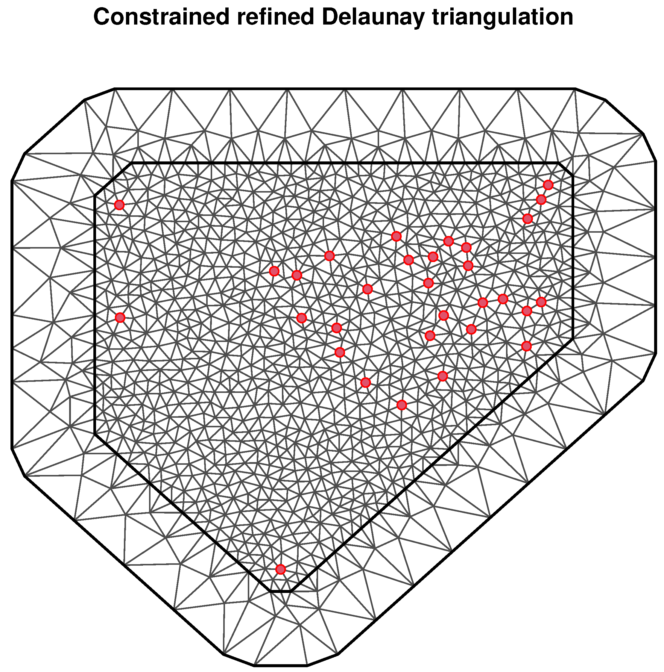
5.3. Implementation of INLA-SPDE

Using INLA-SPDE to fit the model (15), we first need to triangulate mainland China. The function $inla.mesh.2d\left(\right)$ is used for triangulation, where the initial mesh vertex value is the location coordinates after the projection (red dots in the figure), the meshing effect is shown in Figure 2. Then, we use the function $inla.spde2.matern\left(\right)$ to construct the SPDE model and function $inla.spde.make.index\left(\right)$ to create the index set, in order to link the random effects to the observations. Now, we need to use the $inla.spde.make.A\left(\right)$ function to construct a projection matrix A for projecting spatially continuous Gaussian random fields from observations to grid nodes.

After doing these preparations, we can use the function $inla.stack\left(\right)$ to build a stack for uniting the data, effects and projection matrix. The key code is as follows:

$$\begin{array}{c}stack.est<-inla.stack(tag=“est”,data=\dots ,A=\dots ,\\ effects=\dots ,indexs,ID.slm=\dots ).\end{array}$$

It is important to note that $data$ in the code is the response variable, A is the list of the projection matrix. The list of data in $effect$ includes fixed and other random effects, $ID.slm$ is the index of spatial adjacency matrix W.

In order to build the model fitting formulation, we first apply the equation $f1$ consisting of patients with TB and covariate data to construct the spatial lag matrix $mmatrix$. Then, in equation $f2$, only the random effect term is retained, and the matrix parameter X in the $slm$ model is set to the $mmatrix$ established above. The key code for this process is as follows:

$$\begin{array}{c}f1<-y-1+x_1+\dots +x_7\\ mmatrix<-model.matrix(f1,data)\\ f2<-y\sim -1+f(s,model=spde)+\\ f(ID.slm,model=‘slm’,args.slm=list(X=mmatrix,\dots ),hyper=\dots ).\end{array}$$

Finally, the model is fitted by calling the function $inla\left(\right)$ and using the default prior in R-INLA.

5.4. Model Selection

The comparison results of the obtained DIC and WAIC values are shown in

Table 6. Comparison of model evaluation metrics for models (14) and (15).

Model	DIC	WAIC
Model (14)	13,522.22	30,495.35
Model (15)	2117.16	2070.45

.

It can be found out that the DIC value (2117.16) as well as the WAIC value (2070.45) of model (15) is smaller than model (14), indicating that model (15) has better model fitting effect and can fully capture the spatial effects on response variables.

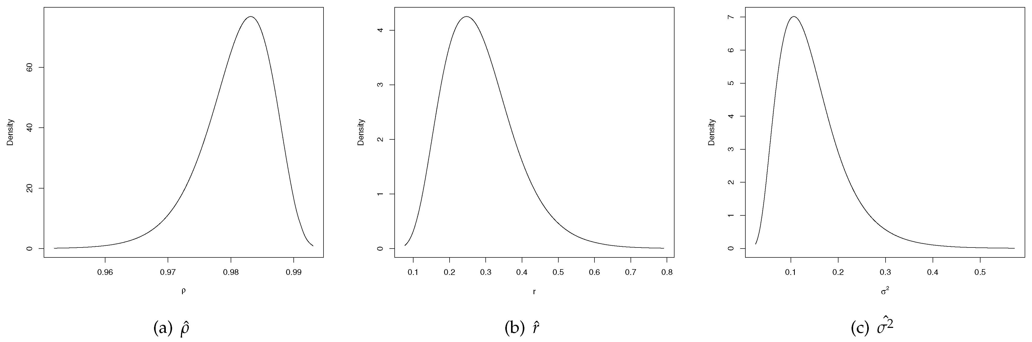
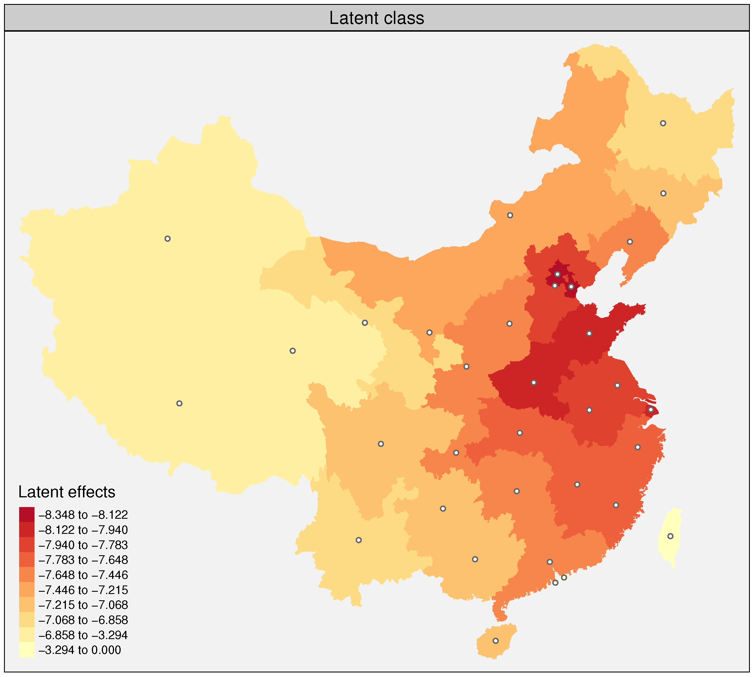
5.5. Model Fitting Results

Using INLA-SPDE to fit model (14) and model (15), the posterior estimations of the fixed effect coefficients are presented in

Table 7. Posterior estimates of the fixed effects coefficients.

Model	Covariates	Mean	SD	0.025 Quantile	0.975 Quantile
Model 14	Precipitation	0.0320	0.0020	0.0280	0.0360
	Temperature	−0.0820	0.0020	−0.0860	−0.0780
	Economy	0.0840	0.0130	0.0600	0.1090
	Medical care	−0.0810	0.0160	−0.1130	−0.0500
	Transportation	−0.1340	0.0090	−0.1510	−0.1180
	Modernization	0.0420	0.0010	0.0400	0.0430
	Particulate Matter	0.0120	0.0030	0.0060	0.0180
Model 15	Precipitation	0.0778	0.0217	0.0351	0.1202
	Temperature	−0.0137	0.0019	−0.0180	−0.0088
	Economy	−0.0191	0.0871	−0.1881	0.1542
	Medical care	−0.1319	0.0539	−0.2398	−0.0273
	Transportation	−0.0366	0.0386	−0.1134	0.0383
	Modernization	−0.0595	0.0375	−0.1330	0.0142
	Particulate Matter	0.0396	0.0113	0.0174	0.0618

.

From Table 7, in the results of model (14), it can be found that the posterior 95% credible intervals for the fixed effects do not contain 0, indicating that they all have a significant effect on the prevalence of TB of different regions. The posterior mean of precipitation, economy, modernization and particulate matter are 0.0320, 0.0840, 0.0420 and 0.0120, respectively, indicating that these factors have significant positive effects on the prevalence of TB. The posterior mean of temperature, medical care and transportation are −0.0820, −0.0810 and −0.1340, respectively, indicating that these three factors have significant negative effects on the prevalence of TB.

However, as model (15) estimated by INLA-SPDE, the spatial autocorrelation parameter of it is $\rho$ = 0.9808 (95%CI:0.9674 0.9897), which indicates that there is a significant spatial dependence between the prevalence of TB of neighboring provinces. The fitting results for model (15) show that the 95% credible intervals of economy, transportation and modernization contain 0, indicating that the effect of these factors is not significant. This may be due to the fact that under the influence of the prevalence of TB in the surrounding areas, the prevalence of TB should have declined significantly as a result of continuous socio-economic and social modernization development and better access to transportation, leading to the improvement of medical standards. However, in reality, the deterioration of the urban environment and the increasing concentration of particulate matter in the air will lead to a further increase in the prevalence of TB. Therefore, we believe that the economy, modernization and transportation should have a differentiated rather than a linear effect on the prevalence of TB.

Fitting curves for parameter $\rho$, r and ${\sigma }^2$, the latent effect for the latent class and the projection of spatial random effect mean and standard deviation are shown in Figure 3, Figure 4 and Figure 5.

For the spatial random effects, the left panel in Figure 5 shows that there is a spatial random effect on the prevalence of TB in China, but it is uneven, which indicates that the covariates in model (15) do not fully account for the spatial effects of TB prevalence; therefore, we may need to add more influences to it for further analysis. The right panel shows the spatial random effects standard deviation; the values of it are related to the distance between different locations, and for locations with large standard deviation values, we can use more data for accurate analysis.

6. Disscussion

When processing and analyzing geostatistic data or other spatial problems, the effects of spatial dependence and spatial heterogeneity cannot be ignored. In this paper, a new latent Bayesian spatial model is proposed to better take into account the spatial dependence of subjects and spatial random effects. We simulate the proposed model under different arithmetic cases separately and have the applicability and limitation that our proposed model is fitted with high precision parameter estimatimation in large samples and significant spatial autocorrelation problems. Then, we applied our model to the TB incidence data in China under INLA-SPDE, and found that the prevalence of TB has strong spatial dependence and non-uniform spatial random effects in mainland China.

Since this paper focuses on the effects of spatial dependence of subjects and heterogeneity of space itself on the response terms, the non-significant covariate effects in the results are not further investigated, while the spatial lag of the covariates themselves and the spatial autocorrelation of the error terms are not extensively considered in more detail. In the future, researchers can continue to build on this study by exploring how INLA-SPDE can be used to incorporate smoothing covariate effects in the latent classes within a Bayesian framework to further analyze the non-significant effects in the results that are already available, as well as investigating the model’s relationship with any other autocorrelation effects.

Finally, one limitation of our study is that the model used in our analysis only includes the spatial structure of the data and does not consider the temporal structure of the data. Data with a spatio-temporal structure would allow the application of INLA-SPDE to spatio-temporal modeling, which would include covariates that may vary in space and time, as well as modeling the random effects of spatio-temporal variation residuals random effects. This would allow us to obtain the effects of spatio-temporal mixed effects on diseases such as TB. However, it is also important to note that spatio-temporal econometric modeling is also a complex problem that requires further investigation.

References

1. Gilks, W.R.; Richardson, S.; Spiegelhalter, D. Markov Chain Monte Carlo in Practice; CRC Press: Boca Raton, FL, USA, 1995. [Google Scholar]
2. Rue, H.; Martino, S.; Chopin, N. Approximate Bayesian inference for latent Gaussian models by using integrated nested Laplace approximations. J. R. Stat. Soc. Ser. B Stat. Methodol. 2009, 71, 319–392. [Google Scholar] [CrossRef]
3. Congdon, P. Bayesian model choice based on Monte Carlo estimates of posterior model probabilities. Comput. Stat. Data Anal. 2006, 50, 346–357. [Google Scholar] [CrossRef]
4. Green, P.J.; Łatuszyński, K.; Pereyra, M.; Robert, C.P. Bayesian computation: A summary of the current state, and samples backwards and forwards. Stat. Comput. 2015, 25, 835–862. [Google Scholar] [CrossRef]
5. Llorente, F.; Martino, L.; Delgado, D.; López-Santiago, J. On the computation of marginal likelihood via MCMC for model selection and hypothesis testing. In Proceedings of the 2020 28th European Signal Processing Conference (EUSIPCO), Amsterdam, The Netherlands, 18–21 January 2021; pp. 2373–2377. [Google Scholar]
6. Llorente, F.; Martino, L.; Delgado, D.; Lopez-Santiago, J. Marginal likelihood computation for model selection and hypothesis testing: An extensive review. SIAM Rev. 2023, 65, 3–58. [Google Scholar] [CrossRef]
7. Lindgren, F.; Rue, H.; Lindström, J. An explicit link between Gaussian fields and Gaussian Markov random fields: The stochastic partial differential equation approach. J. R. Stat. Soc. Ser. B Stat. Methodol. 2011, 73, 423–498. [Google Scholar] [CrossRef]
8. Matérn, B. Spatial Variation; Springer: New York, NY, USA, 1960. [Google Scholar]
9. Rue, H.; Held, L. Gaussian Markov Random Fields: Theory and Applications; CRC Press: Boca Raton, FL, USA, 2005. [Google Scholar]
10. Cameletti, M.; Lindgren, F.; Simpson, D.; Rue, H. Spatio-temporal modeling of particulate matter concentration through the SPDE approach. AStA Adv. Stat. Anal. 2013, 97, 109–131. [Google Scholar] [CrossRef]
11. Moraga, P.; Dean, C.; Inoue, J.; Morawiecki, P.; Noureen, S.R.; Wang, F. Bayesian spatial modelling of geostatistical data using INLA and SPDE methods: A case study predicting malaria risk in Mozambique. Spat.-Spatio-Temporal Epidemiol. 2021, 39, 100440. [Google Scholar] [CrossRef] [PubMed]
12. Moraga, P. Species Distribution Modeling using Spatial Point Processes: A Case Study of Sloth Occurrence in Costa Rica. R J. 2021, 12, 293–310. [Google Scholar] [CrossRef]
13. Zhang, Z.; Krainski, E.; Zhong, P.; Rue, H.; Huser, R. Joint modeling and prediction of massive spatio-temporal wildfire count and burnt area data with the INLA-SPDE approach. Extremes 2023, 26, 339–351. [Google Scholar] [CrossRef]
14. Wilson, B. Evaluating the INLA-SPDE approach for Bayesian modeling of earthquake damages from geolocated cluster data. arXiv 2020. [Google Scholar] [CrossRef]
15. Lindgren, F.; Rue, H. Bayesian spatial modelling with R-INLA. J. Stat. Softw. 2015, 63, 1–25. [Google Scholar] [CrossRef]
16. Krainski, E.T.; Gómez-Rubio, V.; Bakka, H.; Lenzi, A.; Castro-Camilo, D.; Simpson, D.; Lindgren, F.; Rue, H. Advanced Spatial Modeling with Stochastic Partial Differential Equations Using R and INLA; CRC Press: Boca Raton, FL, USA, 2018. [Google Scholar]
17. Anselin, L. Spatial Econometrics: Methods and Models; Springer Science & Business Media: Berlin/Heidelberg, Germany, 1988; Volume 4. [Google Scholar]
18. LeSage, J.; Pace, R.K. Introduction to Spatial Econometrics; CRC Press: Boca Raton, FL, USA, 2009. [Google Scholar]
19. Bivand, R.S.; Gómez-Rubio, V.; Rue, H. Approximate Bayesian inference for spatial econometrics models. Spat. Stat. 2014, 9, 146–165. [Google Scholar] [CrossRef]
20. Bivand, R.; Gómez-Rubio, V.; Rue, H. Spatial data analysis with R-INLA with some extensions. J. Stat. Softw. 2015, 63, 1–31. [Google Scholar] [CrossRef]
21. Hoeting, J.A.; Madigan, D.; Raftery, A.E.; Volinsky, C.T. Bayesian model averaging: A tutorial (with comments by M. Clyde, David Draper and EI George, and a rejoinder by the authors. Stat. Sci. 1999, 14, 382–417. [Google Scholar] [CrossRef]
22. Gómez-Rubio, V.; Palmí-Perales, F. Multivariate posterior inference for spatial models with the integrated nested Laplace approximation. J. R. Stat. Soc. Ser. C Appl. Stat. 2019, 68, 199–215. [Google Scholar] [CrossRef]
23. Gómez-Rubio, V.; Bivand, R.S.; Rue, H. Bayesian model averaging with the integrated nested laplace approximation. Econometrics 2020, 8, 23. [Google Scholar] [CrossRef]
24. Teng, J.; Ding, S.; Shi, X.; Zhang, H.; Hu, X. MCMCINLA Estimation of Missing Data and Its Application to Public Health Development in China in the Post-Epidemic Era. Entropy 2022, 24, 916. [Google Scholar] [CrossRef]
25. Gómez-Rubio, V.; Bivand, R.S.; Rue, H. Estimating spatial econometrics models with integrated nested Laplace approximation. Mathematics 2021, 9, 2044. [Google Scholar] [CrossRef]
26. Basile, R.; Durbán, M.; Mínguez, R.; Montero, J.M.; Mur, J. Modeling regional economic dynamics: Spatial dependence, spatial heterogeneity and nonlinearities. J. Econ. Dyn. Control 2014, 48, 229–245. [Google Scholar] [CrossRef]
27. Blangiardo, M.; Cameletti, M. Spatial and spatio-temporal Bayesian models with R-INLA; John Wiley & Sons: Hoboken, NJ, USA, 2015. [Google Scholar]
28. Hart, P. The condensed nearest neighbor rule (Corresp.). IEEE Trans. Inf. Theory 1968, 14, 515–516. [Google Scholar] [CrossRef]
29. Smirnov, N.V. On the estimation of the discrepancy between empirical curves of distribution for two independent samples. Bull. Math. Univ. Moscou 1939, 2, 3–14. [Google Scholar]
30. Meyer, R. Deviance Information Criterion (DIC). In Wiley StatsRef: Statistics Reference Online; Wiley: Hoboken, NJ, USA, 2016. [Google Scholar]
31. Spiegelhalter, D.J.; Best, N.G.; Carlin, B.P.; Van Der Linde, A. Bayesian measures of model complexity and fit. J. R. Stat. Soc. Ser. b Stat. Methodol. 2002, 64, 583–639. [Google Scholar] [CrossRef]
32. Watanabe, S.; Opper, M. Asymptotic equivalence of Bayes cross validation and widely applicable information criterion in singular learning theory. J. Mach. Learn. Res. 2010, 11, 3571–3594. [Google Scholar]
33. Gelman, A.; Hwang, J.; Vehtari, A. Understanding predictive information criteria for Bayesian models. Stat. Comput. 2014, 24, 997–1016. [Google Scholar] [CrossRef]
34. Roos, M.; Held, L. Sensitivity analysis in Bayesian generalized linear mixed models for binary data. Bayesian Anal. 2011, 6, 259–278. [Google Scholar] [CrossRef]
35. Li, X.X.; Wang, L.X.; Zhang, J.; Liu, Y.X.; Zhang, H.; Jiang, S.W.; Chen, J.X.; Zhou, X.N. Exploration of ecological factors related to the spatial heterogeneity of tuberculosis prevalence in PR China. Glob. Health Action 2014, 7, 23620. [Google Scholar] [CrossRef] [PubMed]
36. Sun, W.; Gong, J.; Zhou, J.; Zhao, Y.; Tan, J.; Ibrahim, A.N.; Zhou, Y. A spatial, social and environmental study of tuberculosis in China using statistical and GIS technology. Int. J. Environ. Res. Public Health 2015, 12, 1425–1448. [Google Scholar] [CrossRef] [PubMed]
37. Moran, P.A. Notes on continuous stochastic phenomena. Biometrika 1950, 37, 17–23. [Google Scholar] [CrossRef]
Figure 1. The fitted plots of ρ , r, σ 2 for n = 300 with different positive autocorrelations.
Mathematics 11 04193 g001
Figure 2. Map of mainland China triangulated grid schematic.
Mathematics 11 04193 g002
Figure 3. The fitted plots of ρ , r and σ 2 in estimation. (a) Posterior marginal of the spatial autocorrelation parameter ρ . (b) Posterior marginal of the separation distance r. (c) Posterior marginal of the marginal variance σ 2 .
Mathematics 11 04193 g003
Figure 4. Posterior means of the latent effect for the latent class.
Mathematics 11 04193 g004
Figure 5. The projection of spatial random effect mean and standard deviation.
Mathematics 11 04193 g005