Order Book Dynamics with Liquidity Fluctuations: Asymptotic Analysis of Highly Competitive Regime

Abstract

We introduce a class of Markov models to describe the bid–ask price dynamics in the presence of liquidity fluctuations. In a highly competitive regime, the spread evolution belongs to a class of Markov processes known as a population process with uniform catastrophes. Our mathematical analysis focuses on establishing the law of large numbers, the central limit theorem, and large deviations for this catastrophe-based model. Large deviation theory allows us to illustrate how huge deviations in the spread and prices can occur in the model. Moreover, our research highlights how these local trends and volatility are influenced by the typical values of the bid–ask spread. We calibrated the model parameters using available high-frequency data and conducted Monte Carlo numerical simulations to demonstrate its ability to reasonably replicate key phenomena in the presence of liquidity fluctuations.

1. Introduction

The “order book” (OB) refers to an electronic list used to describe the evolution of bid and ask prices and sizes in high-frequency electronic markets, such as NYSE-ARCA, LSE, or NASDAQ. The evolution of the OB results from the interaction of buy and sell orders through a rather complex dynamic process. Order book dynamics has been extensively studied in the market microstructure and econophysics literature ([1,2,3]). More recently, based on empirical characteristics presented in these studies, several models for the evolution of the OB have been proposed, as seen in [4,5,6,7]. These models, which are Markovian queueing systems, primarily focus on the direction of the next price movement and provide good results, offering a more or less clear understanding of price dynamics in conditions of uninterrupted high liquidity, i.e., they assume an abundant availability of limited orders in the OB. In this high liquidity context, the prices are relatively stable with small temporary fluctuations, and the bid and ask sizes at the top of the OB provide valuable information on these short-term price fluctuations.

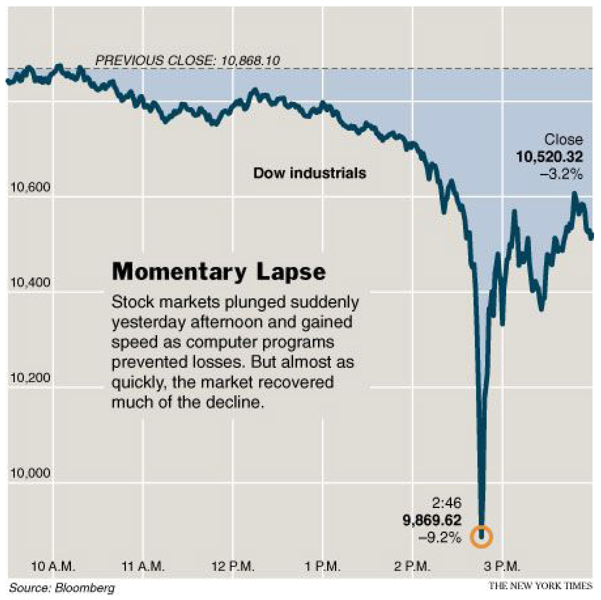
Conversely, in various markets, prices are not as stable; they exhibit significant changes and, in some cases, local downtrends, often caused by liquidity wells in the OB. Events such as the 6 May 2010 “flash crash” (see Figure 1), which was a sudden and severe drop in stock prices in a very short time, have raised concerns about the stability of the OB and its suitability as the primary mechanism for trading. Additionally, occurrences of mini flash crashes—rapid and significantly large directional movements in asset prices—have become increasingly common (see [8]). These events lead to temporary liquidity crises, resulting in larger spreads. Consequently, it is both practically and theoretically important to gain a better understanding of how price dynamics depend on the structure and fundamental parameters of the OB (see [9,10,11]).

Figure 1. A graph of the S&P500 futures on the day of the flash crash of 6 May 2010 at 2:45 p.m.

In the present paper, we are interested in understanding how severe intermittencies in liquidity affect the order book dynamics. The contexts in which there are significant and intermittent decreases in the OB’s ability to absorb market orders are what we call “liquidity fluctuations”. We propose a simple model for price dynamics in an OB with the presence of liquidity fluctuations, our model explains in a simple way how large price fluctuations occur, fluctuations such as those observed in flash crashes. Furthermore, it shows us how these local trends and volatility are determined by the typical values of the bid–ask spread. From our price model, a model for the dynamics of the spread is implicitly derived, we use this model to analyze large deviations in the spread and its impact on prices, we present these large deviations in the form of “optimal trajectories” that give us relevant information about their occurrence. Finally, we present Monte Carlo simulations to corroborate that our model reproduces relevant empirical characteristics observed in our data as well as documented in the literature, such as the famous bid–ask bounce; see [12].

We were initially motivated by the local and seemingly patternless price trends observed in various markets. Our goal was to understand the connection between these long-term trends and the short-term micro-jumps in prices, as shown in Figure 2. Our initial conjecture motivating this work was the existence of a close relationship between the spread, price trends, volatility around these trends, and liquidity fluctuations. Consequently, we needed to jointly model spread and price dynamics. Figure 2 illustrates that the local trend is shared by both bid and ask prices. This observation suggested that our model should not only capture long-term price trends but also incorporate the asymptotically stationary behavior of the spread. Large spread and price changes are typically attributed to liquidity changes ([13]). Our curiosity about this phenomenon grew, leading us to investigate how significant fluctuations in spread and prices, such as those seen in flash crashes, are related to liquidity fluctuations.

Figure 2. Intraday evolution of the ask (red) and bid (green) prices, Apple Inc. (Cupertino, CA, USA) AAPL stock, 4 March 2011. Left: short-term, 1 min. Right: long-term, 15 min. Figures created by H.Rojas.

Our paper is organized as follows. In Section 2, we elucidate key empirical characteristics within an order book exhibiting liquidity fluctuations. We also introduce a general class of continuous-time Markov processes to model bid–ask price dynamics. Section 3 outlines a comprehensive Markovian model for an order book with high liquidity fluctuations. Here, we present the fundamental mathematical statements concerning stability (invariant measure), the law of large numbers, the central limit theorem, and large deviations. In Section 4, we present our numerical results. Section 5 delves into extensions and proposes models for two additional liquidity regimes: non-competitive and low liquidity. Our conclusions are presented in Section 6. The appendix, our final section, contains auxiliary results and proofs of the main statements presented in Section 3.

2. Markov Model and Regimes in Liquidity Fluctuations

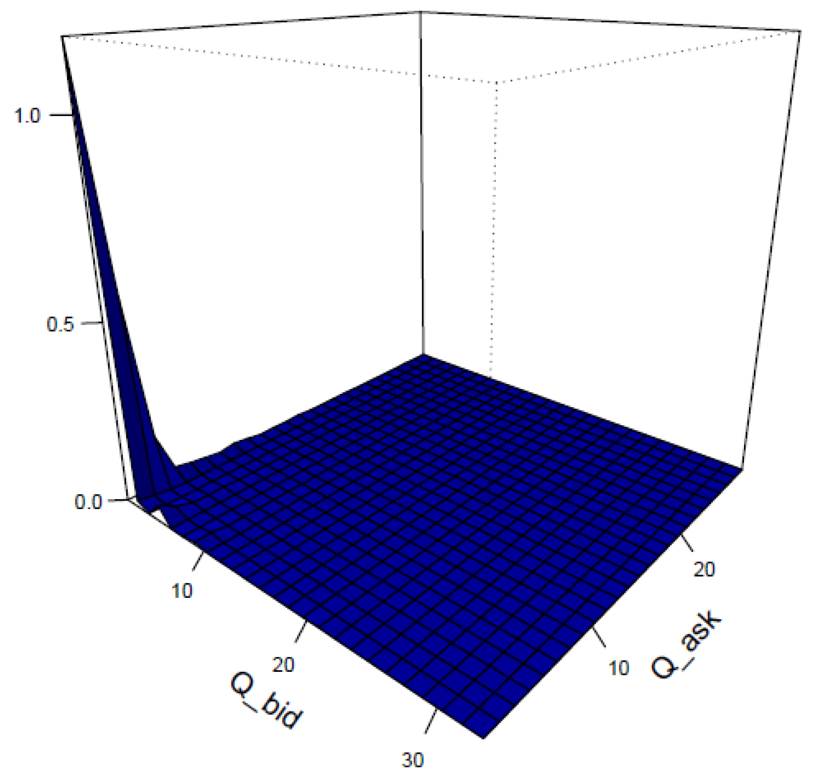
A very important empirical characteristic observed in markets with liquidity fluctuations is the low availability of orders in the OB; the queue sizes at the top of the OB are small most of the time; see, e.g., Figure 3. In this context, the queue sizes of the best bid and ask prices are no longer the determining factors in the dynamics of prices; for more details see [13]. If the liquidity intermittency is severe, even “gaps” are formed in the OB (blocks of adjacent price levels that do not contain quotes). In these cases, the distribution of price changes is mainly determined by the distribution of the gap sizes in the OB. Taking these facts into account, if our interest is to explain the observed long-term price trends, we can focus only on micro-jumps in prices and disregard the size of the queues.

Figure 3. Joint empirical distribution of bid and ask queue sizes at the top of the order book; Apple Inc. stock, 4 March 2011. Figure created by H.Rojas.

In these liquidity regimes, the spread exhibits a quite flexible dynamic behavior, reaching values much larger than those observed in high liquidity conditions; see, e.g., Figure 4. Based on our empirical experiences, the OB slowly digests liquidity fluctuations and we can characterize that process in two stages. In the first stage, the spread begins to increase persistently. In the later stage, the spread is reduced; the reduction can be drastic or gradual. The closing type of the spread in the second stage depends on the intensity of the liquidity fluctuation.

Figure 4. Empirical distribution of the bid–ask spread, Apple Inc. stock, 4 March 2011, corresponding to 15 min of observation (blue). The invariant distribution is calculated by Formula (6) (red). Figure created by H.Rojas.

Our empirical observations about the reversing process of the bid–ask spread to its typical values, before and after liquidity shocks, have been theoretically corroborated through equilibrium models; see [14]. In this paper, we consider different types of reversing processes of the spread, i.e., we consider three low-liquidity regimes: highly competitive, non-competitive, and low liquidity with gaps. These three regimes correspond to low-liquidity regimes but differ in the closing type of the spread and in the gaps present in the OB.

The Markov Model: A General View

Building upon our discussions in the preceding sections, we propose a simplified model for an order book (OB) with liquidity fluctuations. Let $P_b\left(t\right)$ represent the (best) bid price and $P_a\left(t\right)$ denote the (best) ask price. The state of the OB is characterized by a continuous-time process $X\left(t\right)=\left(P_b\left(t\right),P_a\left(t\right)\right)$, taking values in the discrete state space $\tau \mathbb{Z}\times \tau \mathbb{Z}$ (a two-dimensional lattice). Here, $\tau$ represents the “tick size”, and, as usual, $\mathbb{Z}$ denotes the set of integers.

Here, we aim to elaborate on our choice of employing the set of integers $\mathbb{Z}$ as opposed to restricting ourselves to the set of positive integers. This decision is motivated by several factors. One primary reason is the inherent simplicity that arises from utilizing $\mathbb{Z}$ in terms of mathematical description and subsequent analysis. Introducing boundary conditions, such as reflections, can significantly complicate the analytical process.

Furthermore, an additional rationale behind our choice lies in our focus on analyzing systems characterized by constant parameters. In situations where the price tends towards zero, it is possible that this behavior is driven by changes in the underlying system’s parameters (due to a crisis, for example). In contrast, it might not necessarily be an outcome of the dynamics within a model governed by the same parameters. This consideration underscores our approach to employ $\mathbb{Z}$ for its greater flexibility and relevance to the specific context of our analysis.

For the sake of simplicity, we consider $\mathbb{Z}\times \mathbb{Z}$ as the state space of $X\left(t\right)$, interpreting each state as a multiple of $\tau$. The price process $X\left(t\right)$ manifests piecewise constant sample paths, with transitions corresponding to order book events that trigger price fluctuations (as illustrated in Figure 2). Our objective is to describe the asymptotic behavior of the price process $X\left(t\right)$ arising from numerous micro-jumps.

Based on this simplified representation, consider a continuous-time Markov chain $X\left(t\right)=\left(P_b\left(t\right),P_a\left(t\right)\right)$ with state space $\mathbb{X}\subset \mathbb{Z}\times \mathbb{Z}$

$$\mathbb{X}=\left\{\right(b,a)\in \mathbb{Z}\times \mathbb{Z}:\mathrm{such} \mathrm{that}b<a\}.$$

Here, $P_b\left(t\right)$ represents the bid price, $P_a\left(t\right)$ represents the ask price, and $S\left(t\right)=P_a\left(t\right)-P_b\left(t\right)$ is the bid–ask spread. In general, the transitions of the chain $X\left(t\right)$ are defined by the following transition rates: given a state $(b,a)$, then

$$\begin{array}{cc}\hfill & (b,a)\to (b,a+\Delta )\mathrm{with}\mathrm{rate}{\alpha }_{+}(\Delta ),\hfill \\ \hfill & (b,a)\to (b,a-\Delta )\mathrm{with}\mathrm{rate}{\alpha }_{-}(\Delta ),\mathrm{where}0<\Delta <a-b,\hfill \\ \hfill & (b,a)\to (b-\Delta ,a)\mathrm{with}\mathrm{rate}{\beta }_{-}(\Delta ),\hfill \\ \hfill & (b,a)\to (b+\Delta ,a)\mathrm{with}\mathrm{rate}{\beta }_{+}(\Delta ),\mathrm{where}0<\Delta <a-b,\hfill \end{array}$$

(1)

in all cases, the increment $\Delta$ is a positive integer number. The function ${\alpha }_{+}(·)$ (resp. ${\beta }_{-}(·)$) is the rate at which increases (resp. decreases) in the ask (resp. bid) price occur as a result of the execution of market buy (resp. sell) orders or cancellations of limited sell (resp. buy) orders, as well as, that the function ${\alpha }_{-}(·)$ (resp. ${\beta }_{+}(·)$) is the rate at which the decreases (resp. increases) in the ask (resp. bid) price occur as a result of a limited sell (resp. buy) order placed within the spread.

We study the asymptotic behavior of $X\left(t\right)$ as t goes to infinity. To facilitate this analysis, it is convenient to consider an equivalent process, denoted as $Y\left(t\right)=\left(P_b\left(t\right),S\left(t\right)\right)$ with state space $\mathbb{Y}=\mathbb{Z}\times \mathbb{N}$. Although both $X\left(t\right)$ and $Y\left(t\right)$ contain the same information, the latter representation offers better control for our asymptotic examination. The transitions of the chain $Y\left(t\right)$ are defined by the following transition rates: given a state $(b,s)$ of the Markov chain, then

$$\begin{array}{cccc}\hfill & (b,s)\to (b,s+\Delta )\hfill & \hfill \mathrm{with}\mathrm{rate}& {\alpha }_{+}(\Delta ),\hfill \\ \hfill & (b,s)\to (b,s-\Delta )\hfill & \hfill \mathrm{with}\mathrm{rate}& {\alpha }_{-}(\Delta ),\hfill \\ \hfill & (b,s)\to (b-\Delta ,s+\Delta )\hfill & \hfill \mathrm{with}\mathrm{rate}& {\beta }_{-}(\Delta ),\hfill \\ \hfill & (b,s)\to (b+\Delta ,s-\Delta )\hfill & \hfill \mathrm{with}\mathrm{rate}& {\beta }_{+}(\Delta ).\hfill \end{array}$$

(2)

Since the transition rates of $Y\left(t\right)$ depend only on the second coordinate, the spread, we see that $S\left(t\right)$ alone is the continuous-time Markov process and has the following transition rates. Suppose that at some moment the spread is $k\in \mathbb{N}$, then

$$\begin{array}{cccc}\hfill k& \to k+\Delta \hfill & \hfill \mathrm{with} \mathrm{rate}& {\gamma }_{+}(\Delta ):={\alpha }_{+}(\Delta )+{\beta }_{-}(\Delta ),\hfill \\ \hfill k& \to k-\Delta \hfill & \hfill \mathrm{with} \mathrm{rate}& {\gamma }_{-}(\Delta ):={\alpha }_{-}(\Delta )+{\beta }_{+}(\Delta ).\hfill \end{array}$$

(3)

Based on the model (1) and its alternative representation (2) and (3), it is possible to define three low-liquidity regimes: highly competitive, non-competitive, and low liquidity with gaps. Any regime is defined by how the rates depend on the increment $\Delta$ which is usually determined by the intensity of the liquidity fluctuations.

In this paper, our focus is primarily on the first regime, namely, the highly competitive regime, while the other two regimes are outlined briefly. The findings presented here can be generalized for the other two regimes, but we believe that there will be no significant qualitative difference in the results.

3. The Markov Model: Closing the Spread Uniformly (Highly Competitive Regime)

The highly competitive regime (HC regime) is characterized by very small opening steps of the spread and a rapid decrease in it. This regime is consistent with a rapid reversing process of the spread and the absence of gaps in the order book (OB). The rapid decrease in the spread is caused by the competitive behavior of impatient agents who place quotes within the spread, prioritizing the execution of their placed limit orders. In the considered model (1), we define the rates in such a way that the spread can increase by only one unit. For a given spread length, denoted as k, the next length of the spread is chosen uniformly from the set $I_k=\{1,\cdots ,k-1\}$.

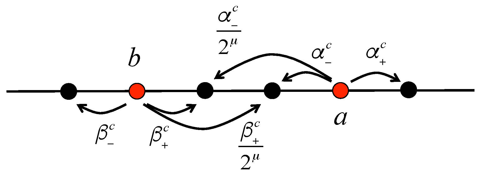
In order to define the rates for the highly competitive regime, we make use of our notation and fix the parameters ${\alpha }_{+}$, ${\alpha }_{-}$, ${\beta }_{+}$, and ${\beta }_{-}$, which are strictly positive real numbers. Furthermore, the terms ${\alpha }_{\pm }$ and ${\beta }_{\pm }$ are employed solely as parameters of the model and not as functions. The transition rates for the Markov chain $X\left(t\right)$ are defined as follows: given that the chain is in a state $(b,a)\in \mathbb{X}$ at a certain moment, then

$$\begin{array}{c}\hfill {\alpha }_{+}(\Delta )=\left\{\begin{array}{cc}\hfill {\alpha }_{+},& \mathrm{if} \Delta =1;\hfill \\ \hfill 0,& \mathrm{otherwise};\hfill \end{array}\right.{\alpha }_{-}(\Delta )=\left\{\begin{array}{cc}\hfill \frac{{\alpha }_{-}}{ a-b-1},& \mathrm{if} a-b>1 \mathrm{for} \mathrm{any} \Delta \in I_{a-b};\hfill \\ \hfill 0,& \mathrm{otherwise};\hfill \end{array}\right.\\ \hfill {\beta }_{-}(\Delta )=\left\{\begin{array}{cc}\hfill {\beta }_{-},& \mathrm{if} \Delta =1;\hfill \\ \hfill 0,& \mathrm{otherwise};\hfill \end{array}\right.{\beta }_{+}(\Delta )=\left\{\begin{array}{cc}\hfill \frac{{\beta }_{+}}{a-b-1},& \mathrm{if} a-b>1 \mathrm{for} \mathrm{any} \Delta \in I_{a-b};\hfill \\ \hfill 0,& \mathrm{otherwise}.\hfill \end{array}\right.\end{array}$$

(4)

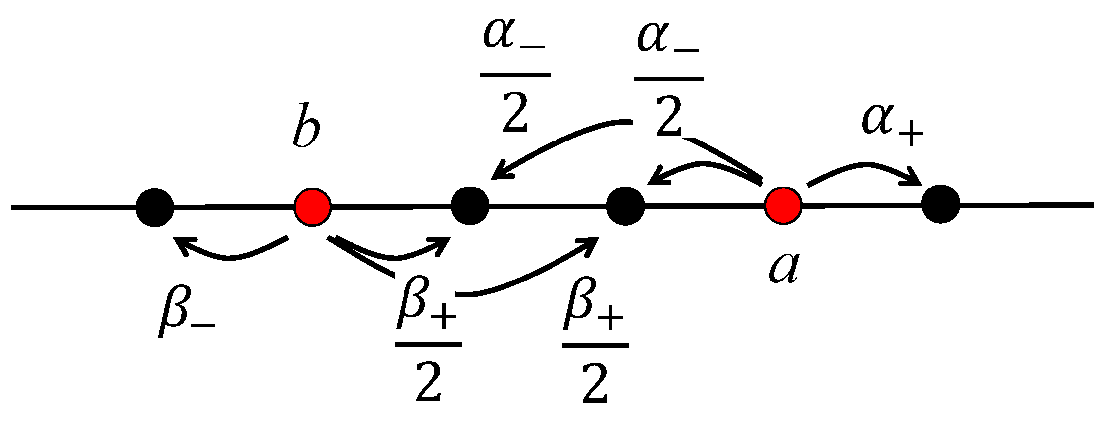
For an illustration, see Figure 5 in the case when $a-b=3$.

Figure 5. The rates for the highly competitive model. An illustrative example of the case when $a-b=3$. Figure created by A.Yambartsev.

In this regime, the transition rates of $S\left(t\right)$, see (3), are the following: suppose that at some moment the spread is $k\in \mathbb{N}$, and let ${\gamma }_{+}:={\beta }_{-}+{\alpha }_{+}$ and ${\gamma }_{-}:={\beta }_{+}+{\alpha }_{-}$, then

$$\begin{array}{cccc}\hfill k& \to k+1\hfill & \hfill \mathrm{with} \mathrm{rate}& {\gamma }_{+},\hfill \\ \hfill k& \to k-\Delta \hfill & \hfill \mathrm{with} \mathrm{rate}& \frac{{\gamma }_{-}}{k-1} \mathrm{for} \Delta \in I_k.\hfill \end{array}$$

(5)

Note that $S\left(t\right)$ is an irreducible Markov chain in this regime.

3.1. Ergodicity and Invariant Measure for $S\left(t\right)$

We begin by analyzing the stability of the spread $S\left(t\right)$. The following theorem establishes ergodicity, representing one of the rare instances where we are able to determine the invariant measure for the process.

Theorem 1.

In a highly competitive regime model, for any positive values of parameters ${\alpha }_{+},{\alpha }_{-},{\beta }_{+},$${\beta }_{-}$ the spread $S\left(t\right)$ is a positive recurrent Markov process with an invariant measure denoted as $\mu =\left(\mu \left(k\right),k\in \mathbb{N}\right)$ given by the following formula: let $\gamma :={\gamma }_{+}+{\gamma }_{-}$

$$\mu \left(k\right)=\frac{k!{\left({\gamma }_{+}\right)}^{k-1}}{{\prod }_{i=1}^{k-1}({\gamma }_{-}+i\gamma )}{\left(1+\sum _{k\ge 2}\frac{k!{\left({\gamma }_{+}\right)}^{k-1}}{{\prod }_{i=1}^{k-1}({\gamma }_{-}+i\gamma )}\right)}^{-1}.$$

(6)

These findings regarding the stationary asymptotic behavior of the spread process $S\left(t\right)$ are in line with the empirical observations illustrated in Figure 4.

We conclude this section with the following observation: the process $S\left(t\right)$ falls within the category of processes referred to as population processes with uniform catastrophes. An extension to processes with almost uniform catastrophes (as defined in Section 5.1) was explored in [15]. In that work, the following result was established for the maximum of the process: for any fixed $b\in (0,1)$

$$\mathbb{P}\left(\underset{T\to \infty }{lim}\underset{t\in [0,1]}{sup}\frac{S\left(tT\right)}{T^b}>\epsilon \right)=0.$$

3.2. Local Drift (LLN for the Prices)

The following theorem addresses the law of large numbers (LLN) as applied to prices. This theorem will illuminate the local trends (local drift) exhibited by the prices.

Theorem 2.

With probability one scaled by the time the bid price converges to a constant

$$\frac{P_b\left(t\right)}{t}\to D\mathrm{a}.\mathrm{s}.t\to \infty ,$$

(7)

where

$$D=-{\beta }_{-}-\mu \left(1\right)\gamma \left(\frac{{\beta }_{-}{\gamma }_{-}}{{\gamma }_{+}}+\frac{{\beta }_{+}}{2}\right)+\frac{{\beta }_{+}\gamma }{2}\sum _{k\ge 1}k\mu \left(k\right).$$

This result validates our conjecture regarding the impact of the spread on the local trend of prices. From a practical standpoint, given the jump rates of the bid and ask prices, we can easily compute the price trend.

3.3. Price Volatility (CLT for the Prices)

In this section, our focus is on examining the connection between price volatility and price jump rates. Specifically, we establish a central limit theorem (CLT) for the price process. We articulate the volatility of price fluctuations around local drift in relation to the jump rates of the ask and bid prices. In other words, the central limit theorem holds for the process depicted by (A3).

Once more, we begin by demonstrating the central limit theorem (CLT) for the embedded discrete-time dynamics $p_n$ of the price (Lemma 1), followed by establishing the CLT for the continuous-time chain $P_b\left(t\right)$ (Theorem 3). We have included the proofs in the Appendix A.

Lemma 1.

Let $n\to \infty$, then

$$\frac{p_n-nv}{\sqrt{n\mathbb{V}a{r}_{\widehat{\pi }}\left(F\left({\widehat{s}}_n\right)\right)}}\to N(0,1)$$

in distribution, where

$$\mathbb{V}a{r}_{\widehat{\pi }}\left(F\left({\widehat{s}}_n\right)\right)=\frac{{\beta }_{-}}{\gamma }+\frac{\mu \left(1\right)}{\gamma }\left(\frac{{\beta }_{-}{\gamma }_{-}}{{\gamma }_{+}}-\frac{{\beta }_{+}}{6}\right)+\frac{{\beta }_{+}}{\gamma }\frac{1}{6}\sum _{s=1}^{\infty }s(2s-1)\pi \left(s\right)-{\left[{\mathbb{E}}_{\widehat{\pi }}\left(F\left({\widehat{s}}_n\right)\right)\right]}^2$$

Lemma 1 establishes a connection between the “coarse-grained” volatility of intraday returns at lower frequencies and the high-frequency jump rates of prices. In simpler terms, it asserts that prices exhibit a diffusive behavior around a local drift over time, with a diffusion coefficient of $\mathbb{V}a{r}_{\widehat{\pi }}\left(F\left({\widehat{s}}_n\right)\right)$. Consequently, price volatility, as determined by the number of micro-jumps in prices, is given by

$${\sigma }_n=\sqrt{n\mathbb{V}a{r}_{\widehat{\pi }}\left(F\left({\widehat{s}}_n\right)\right)}$$

(8)

Here, n represents the total count of high-frequency price jumps. Equation (8) presents a means to estimate price volatility without requiring long-term price observations. Optionally, the parameter ${\sigma }_n$ can be interpreted as the intraday realized volatility of the asset. Thus, relation (8) establishes a link between the realized volatility and the high-frequency parameters of the order book.

Based on Lemma 1, we established Theorem 3; see proof in Appendix A.4. Note that the proof of the law of large numbers provides the following representation for local drift D in continuous time $D=v\gamma$, where v is the local drift for an embedded chain provided by Lemma A1 (see Appendix A.2).

Theorem 3.

Let $t\to \infty$, then there exists ${\sigma }^2>0$ such that

$$\begin{array}{c}\hfill \sqrt{t}\left(\frac{P_b\left(t\right)}{t}-D\right)\to N\left(0,({\sigma }^2+v^2)\gamma \right),\end{array}$$

in distribution.

3.4. Large Deviations for the Spread $S\left(t\right)$

It is known that in the context of liquidity fluctuations, even a small order can trigger a substantial price change, thereby leading to a significant increase in the spread ([3,13]). Consequently, our interest lies in comprehending the mechanisms behind substantial spread changes without altering the model’s parameters. We believe that such analyses can contribute to evaluating the order book’s resilience against severe liquidity fluctuations.

In this section, we present an application of the large deviations theory to the Markov process that describes the dynamics of the spread. Specifically, we investigate the asymptotics of large deviations for the spread process. Our goal is to identify the most probable trajectory associated with a specific state of the spread, particularly when it becomes very large, over a given time interval.

The topic of large deviations for Poisson processes with uniform (or almost uniform) catastrophes has been explored in [15,16]. Large deviation analysis serves as a culminating step within a sequence of limit theorems for such processes. While the theory of large deviations is well-developed, the processes examined here do not satisfy the “classical” conditions. Consequently, the proof of large deviations remains quite technical.

In order to provide the large deviations, we need some increasing scaling parameter. Let T be the length of the time interval $[0,T]$ over which we observe our process. We consider the following scaled process:

$$S_T\left(t\right)=\frac{S\left(tT\right)}{T},t\in [0,1].$$

We say that the family of the random variable $S_T\left(1\right)$ satisfies the large deviation principle (LDP) on $\mathbb{R}$ with the rate function $I=I\left(x\right):\mathbb{R}\to [0,\infty ]$ if for any $c\ge 0$ the set $\{x\in \mathbb{R}:I(x)\le c\}$ is compact and for any set $B\in \mathcal{B}\left(\mathbb{R}\right)$ the following inequalities hold:

$$\underset{T\to \infty }{lim\; sup}\frac{1}{T}ln\mathbb{P}(S_T\left(1\right)\in B)\le -\underset{x\in \left[B\right]}{inf}I\left(x\right)\mathrm{and}\underset{T\to \infty }{lim\; inf}\frac{1}{T}ln\mathbb{P}(S_T\left(1\right)\in B)\ge -\underset{x\in \left(B\right)}{inf}I\left(x\right),$$

where $\mathcal{B}\left(\mathbb{R}\right)$ is the Borel $\sigma$-algebra on $\mathbb{R}$ and $\left[B\right],\left(B\right)$ are the closure and open interior of the set B, respectively. This principle was established in [16], in which the logarithmic asymptotic for the probability $\mathbb{P}(S_T\left(1\right)>x)$ was calculated. Note that the principle was proved for the state x of the spread at the time T, it is not the principle on the functional space. The principle on the functional (trajectory) space provides us the possibility to find the (unique) optimal trajectory—the trajectory which shows how such deviation (a rare event) occurs taking into account the evolution of the spread.

An initial approach to proving the principle in the functional space is to establish the local large deviation, which involves studying the asymptotic behavior of the probability of the process remaining within a small neighborhood of a given continuous function. We say that the family of the processes $S_T(·)$ satisfies the local large deviation principle (LLDP) on the set $G\subset \mathbb{D}[0,1]$ with rate function $I=I\left(f\right):\mathbb{D}[0,1]\to [0,\infty ]$ if for any function $f\in G$ the following inequalities hold:

$$\underset{\epsilon \to 0}{lim}\underset{T\to \infty }{lim\; sup}\frac{1}{T}ln\mathbb{P}(S_T(·)\in U_{\epsilon }\left(f\right))=\underset{\epsilon \to 0}{lim}\underset{T\to \infty }{lim\; inf}\frac{1}{T}ln\mathbb{P}(S_T(·)\in U_{\epsilon }\left(f\right))=-I\left(f\right),$$

where $\mathbb{D}[0,1]$ is the space of càdlàg functions, i.e., the functions that are continuous from the right, and have a limit from the left; and where $U_{\epsilon }\left(f\right):=\{g\in \mathbb{D}[0,1]:{sup}_{t\in [0,1]}|f\left(t\right)-g\left(t\right)|\le \epsilon \}$.

The LLDP was proved in [15] for the compound Poisson process with almost uniform catastrophes. We note only here that the process $S(·)$ is the special case of the processes considered in [15]. Let G be a set of absolutely continuous functions that are positive on the interval (0, 1]. In order to write the corresponding rate function, we need to remember that any function with a finite variation can be uniquely represented as a difference of two non-decreasing functions $f^{+}$ and $f^{-}$ such that $\mathrm{Var}{f}_{[0,1]}=\mathrm{Var}{f}_{[0,1]}^{+}+\mathrm{Var}{f}_{[0,1]}^{-}$. The functions $f^{+}$ and $f^{-}$ are called the positive and negative variations in the function f, respectively. Now, the rate function for $S_T(·)$ can be represented for $f\in G$ as follows:

$$I\left(f\right)={\gamma }_{-}+{\int }_0^1\left({\dot{f}}^{+}\left(t\right)ln\left(\frac{{\dot{f}}^{+}\left(t\right)}{{\gamma }_{+}}\right)-{\gamma }_{+}\left(\frac{{\dot{f}}^{+}\left(t\right)}{{\gamma }_{+}}-1\right)\right)\mathbf{I}\left({\dot{f}}^{+}\left(t\right)>{\gamma }_{+}\right)dt,$$

(9)

where $\dot{f}$ stands for the derivative of function f and $\mathbf{I}$ is the indicator function.

We note that the large deviation principle and local large deviation have the same normalization factor for the probabilities, $1/T$. This provides the existence of an optimal trajectory for the large deviations. The existence of the optimal trajectories of large deviations $S_T\left(1\right)>x$ was established in [16]. If $x<{\gamma }_{+}$, then there exists the moment $t_x=1-\frac{x}{{\gamma }_{+}}\in (0,1)$ such that the spread process $S_T(·)$ stays near zero up to the time $t_x$ and after that $S_T\left(t\right)$, $t\ge t_x$ increases according to the straight line which starts at point $(t_x,0)$ and grows up to the point $(1,x)$ with the slope ${\gamma }_{+}$; see function $f_2$ in Figure 6A. If $x\ge {\gamma }_{+}$, then the process grows together with the straight line starting from the origin up to the point $(1,x)$, i.e., its slope is x; see function $f_1$ in Figure 6A. For illustrative purposes of comparison, in Figure 6 we represent the optimal trajectories that provide large fluctuations for the Poisson process with rate ${\gamma }_{+}$ and the process $S_T$, that is, the Poisson process (of rate ${\gamma }_{+}$) with uniform catastrophes (of rate ${\gamma }_{-}$).

Figure 6. The optimal trajectories for (A) spread process, which is a Poisson process (of rate ${\gamma }_{+}$) with uniform catastrophes (of rate ${\gamma }_{-}$), and (B) Poisson process with rate ${\gamma }_{+}$. If $x<{\gamma }_{+}$, then the large deviation occurs according to the functions $f_2$. If $x\ge {\gamma }_{+}$, then the large deviation trajectory is in the neighborhood of the straight line $f_1$. Figures created by A.Yambartsev.

3.5. Large Deviations for the Prices $(P_b\left(t\right),P_a\left(t\right))$

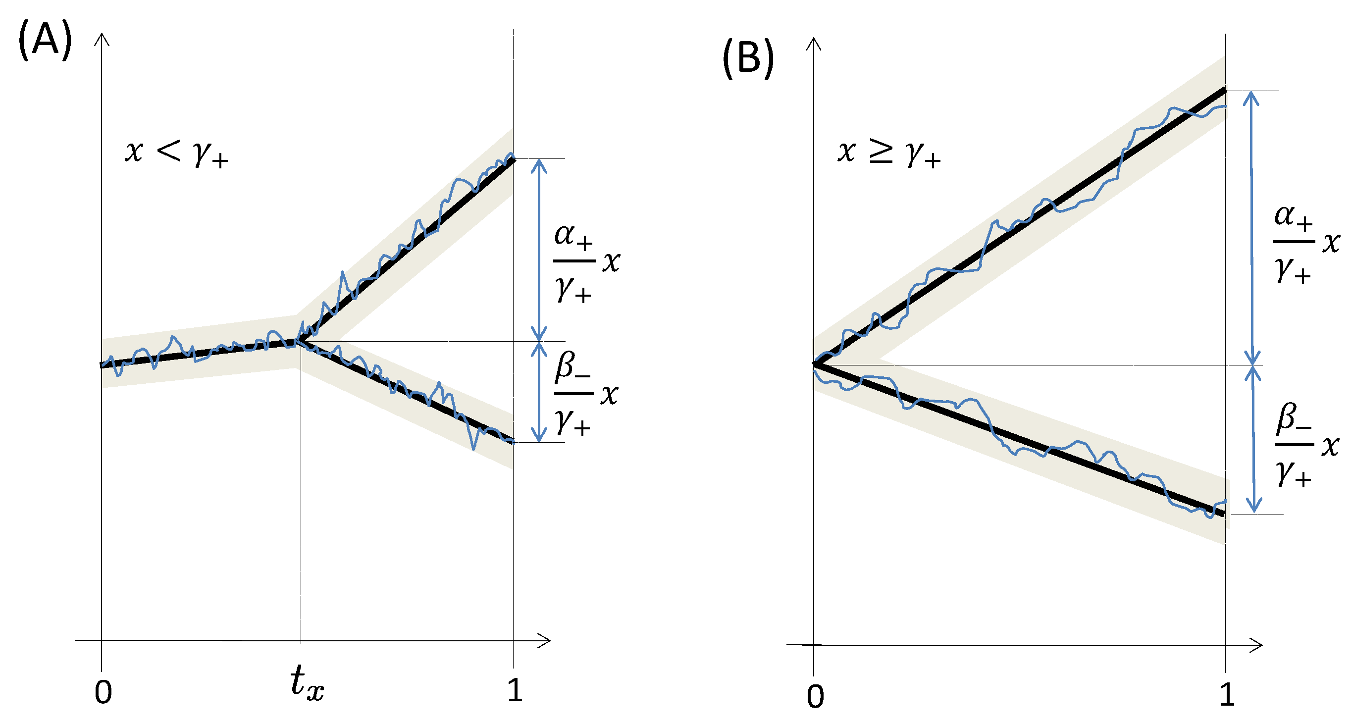
The large deviation result for the spread suggests the question about the behavior of prices under a large spread. The rate function corresponding to the large deviation is essentially the rate function of a Poisson process with rate ${\gamma }_{+}$, which consists of the rates ${\alpha }_{+}$ and ${\beta }_{-}$. Here, we provide some qualitative behavior of optimal price trajectories without proof. The qualitative picture is represented in Figure 7.

Figure 7. The optimal trajectories for prices $(P_b\left(t\right),P_a\left(t\right))$ under a large deviation of the spread when (A) the scaled spread x is less than ${\gamma }_{+}$, which consists of the rates ${\beta }_{-},{\alpha }_{+}$, i.e., ${\gamma }_{+}={\beta }_{-}+{\alpha }_{+}$; and (B) the scaled spread $x\ge {\gamma }_{+}$. Figures created by A.Yambartsev.

The main difference between the behavior of the optimal trajectories of Poisson processes and our process lies in the inclusion of the indicator function within the rate function, as seen in (9). This indicator function imposes a constraint on the possible values of the line slope—it cannot be lower than the rate of the Poisson process. Consequently, when the scaled spread is less than ${\gamma }_{+}$, a “bifurcation” point $t_x$ emerges. After this point, the upper line has a slope of ${\alpha }_{+}$ and the lower line has a slope of $-{\beta }_{+}$. As the scaled spread surpasses ${\gamma }_{+}$, the slopes change, but the relationship between the contributions of rates ${\alpha }_{+}$ and $-{\beta }_{+}$ remains constant.

4. Numerical Simulations and Applications

This section provides a detailed description of the data and the empirical facts relevant to them. We also present computational simulations used to calibrate the model parameters, using the data to validate some qualitative model outcomes. Additionally, we demonstrate a practical application that confirms our model’s short-term predictive capabilities.

4.1. HFT Data

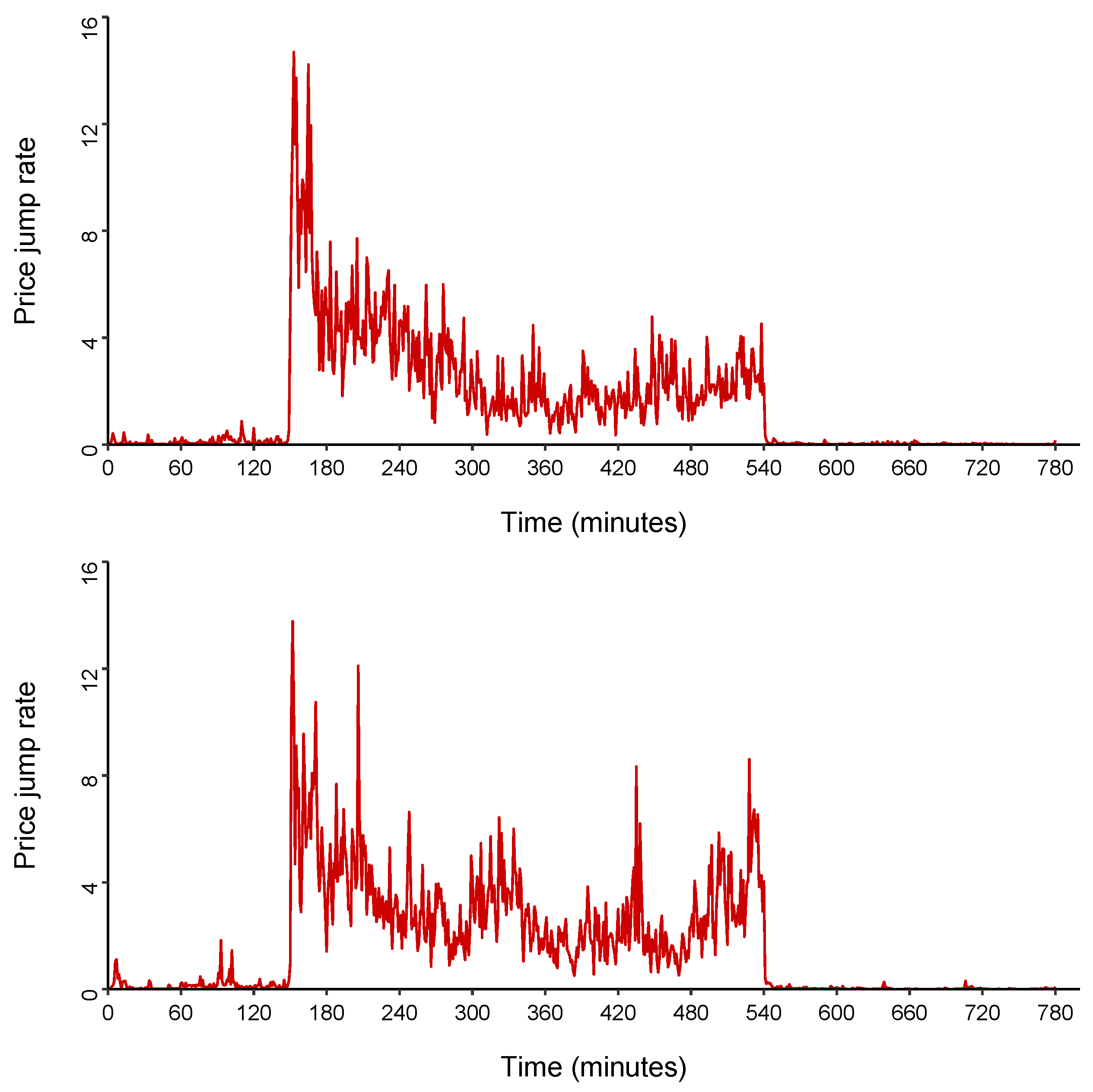
The dataset consists of NASDAQ high-frequency trading (HFT) data for Apple Inc., collected through the Bloomberg stock trading platform. High-frequency data are collected within the day (intraday), and recorded tick by tick. The dataset covers 12 h of trading activity each day, specifically, the entire trading population for 3 and 4 March 2011. During the first 12 h of market operation, the order book quotes, measured by the frequency of price jumps, remain stable for periods ranging from 180 to 540 min after the market opens, as shown in Figure 8. Consequently, for both trading days, we will analyze data from within these time intervals. It is noteworthy that during these intervals there are approximately 305 thousand price jumps per day, a characteristic that typically persists on a daily basis.

Figure 8. Intensity of price jumps: average number of micro-jumps per minute. Upper graph: 3 March 2011. Lower graph: 4 March 2011. Figures created by H.Rojas.

4.2. Empirical and Qualitative Facts

In this section, based on the available data presented above, we present some empirical and qualitative characteristics that are typically observed in high-frequency trading markets. The objective of this section is to corroborate whether the assumptions underlying our model align with these recurring qualitative features commonly found in most markets.

As previously mentioned, our model’s key assumption is that in conditions of low liquidity, characterized by a high intensity of price jumps, the sizes of the bid and ask orders diminish in significance as the primary factors influencing the price dynamics. In contrast, under these conditions, the bid–ask spread becomes the determining factor in predicting price dynamics.

In order to empirically validate this assumption, we will label the observed price variations into two categories: up variations for upward variations, and down variations for downward variations. After binarizing the price jumps, we use them as binary labels (target variable) to classify jumps based on the bid–ask spread and the sizes of the bid and ask orders as predictors.

The idea is that the greater the predictive power, the greater the influence on price dynamics. It is worth mentioning that to measure the predictive power of order sizes, the imbalance was considered, which corresponds to the fraction of the ask size and the sum of total orders, that is, the bid size divided by the sum of the bid and ask sizes.

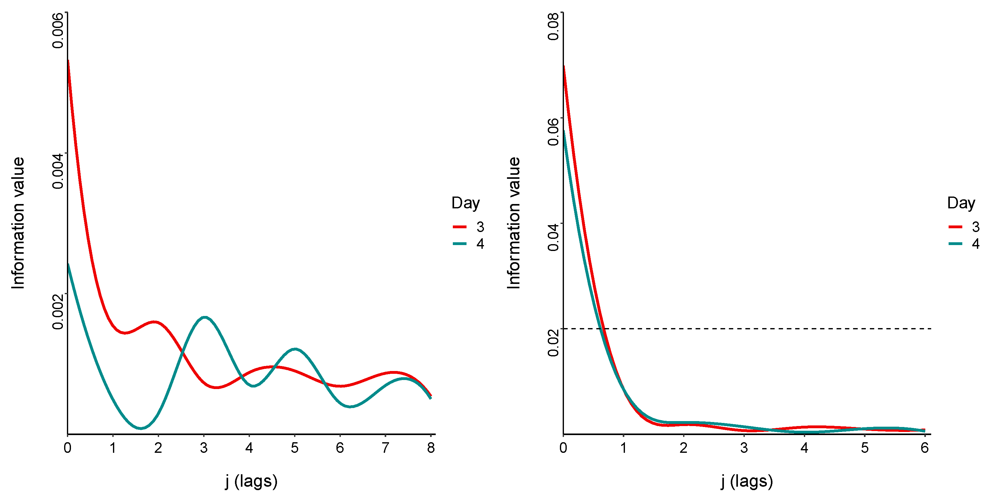
There are various dissimilarity metrics, known as divergence measures in information theory, that we can use to assess the predictive power of the bid–ask spread and the imbalance. Due to its simplicity and wide use in classification problems, we will employ the Jeffreys divergence, also known as the information value (IV); see, for example, reference [17].

Based on the information value (IV) (see Figure 9) we corroborate that the bid–ask spread has a persistent and relevant influence on the price dynamics. On the other hand, the imbalance, and consequently the size of the orders, has an influence that disappears quickly over time. Therefore, our main assumption of the model, the prevailing influence of the spread on price dynamics, is empirically validated in our data. It is worth noting that the influence of the bid–ask spread fluctuates, and our model implicitly accounts for this empirical observation.

Figure 9. The vertical axis corresponds to the information value (IV). The horizontal axis corresponds to the time lag (lags) taken into account for the calculation of the divergence, that is, contiguous periods where price jumps occur. The graph on the left corresponds to the spread bid–ask predictor. The graph on the right corresponds to the imbalance predictor. Figures created by H.Rojas.

4.3. Parameter Estimation and Monte Carlo Experiments

In this section, we explore the steady-state properties of our proposed model using Monte Carlo simulations. We compare the empirically observed long-term behavior (unconditional properties) of the OB to simulations of the fitted model. The goal of these simulations is to indicate how well the model reproduces the average properties of the OB. The transition rates of $X\left(t\right)$ can be estimated by

$${\widehat{\alpha }}_{+}=\frac{N_{{\alpha }_{+}}}{T},{\widehat{\alpha }}_{-}=\frac{N_{{\alpha }_{-}}}{T},{\widehat{\beta }}_{+}=\frac{N_{{\beta }_{+}}}{T},{\widehat{\beta }}_{-}=\frac{N_{{\beta }_{-}}}{T},$$

(10)

where T is the length of our sample (in seconds), $N_{{\alpha }_{+}}$ ($N_{{\alpha }_{-}}$) is the total number of jumps where the ask price increases (decreases), and $N_{{\beta }_{+}}$ ($N_{{\beta }_{-}}$) is the total number of jumps where the bid price increases (decreases).

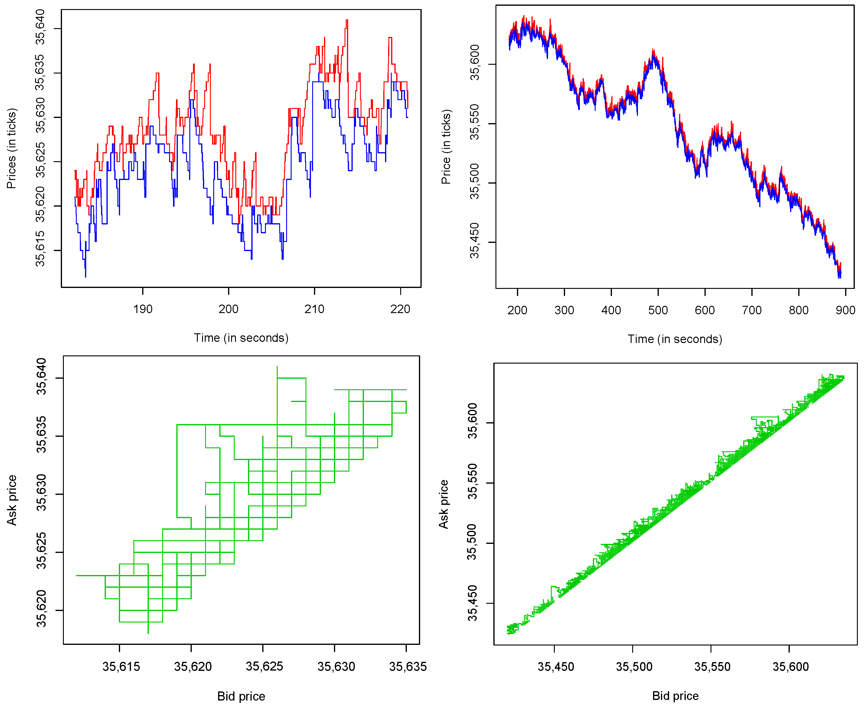
From the Apple stock data, since our model (4) only allows spread openings in one tick, we selected approximately 15 continuous minutes of trading for which spread openings only occurred in one tick, which corresponds to the interval of 365 to 380 min after the market opens. In this sub-sample, using (10), we obtain the following: $T=900$ s, ${\widehat{\alpha }}_{+}=3.756$, ${\widehat{\alpha }}_{-}=0.765$, ${\widehat{\beta }}_{+}=0.848$, and ${\widehat{\beta }}_{-}=4.907$. Based on the estimation of the parameters $({\widehat{\alpha }}_{+},{\widehat{\alpha }}_{-},{\widehat{\beta }}_{+},{\widehat{\beta }}_{-})$, we simulate the price process $X\left(t\right)$ over a long horizon of 900 s, which corresponds to what was empirically observed, and observe the evolution of prices in two time windows. The results are displayed in Figure 10. The results of our simulations illustrate that our model reproduces realistic characteristics for both the short- and long-term price behavior, which were presented for the empirical data in Figure 2.

Figure 10. Simulation of the order book with parameters ${\widehat{\alpha }}_{+}=3.756$, ${\widehat{\alpha }}_{-}=0.765$, ${\widehat{\beta }}_{+}=0.848$, and ${\widehat{\beta }}_{-}=4.907$. Upper left: Short-term evolution of bid (blue) and ask (red) prices, 1 min sample. Upper right: Long-term evolution of the prices, 15 min sample. Bottom left: short-term path of the price process $X\left(t\right)$, 1 min sample. Bottom right: long-term path of the price process, 15 min sample. Figures created by H.Rojas.

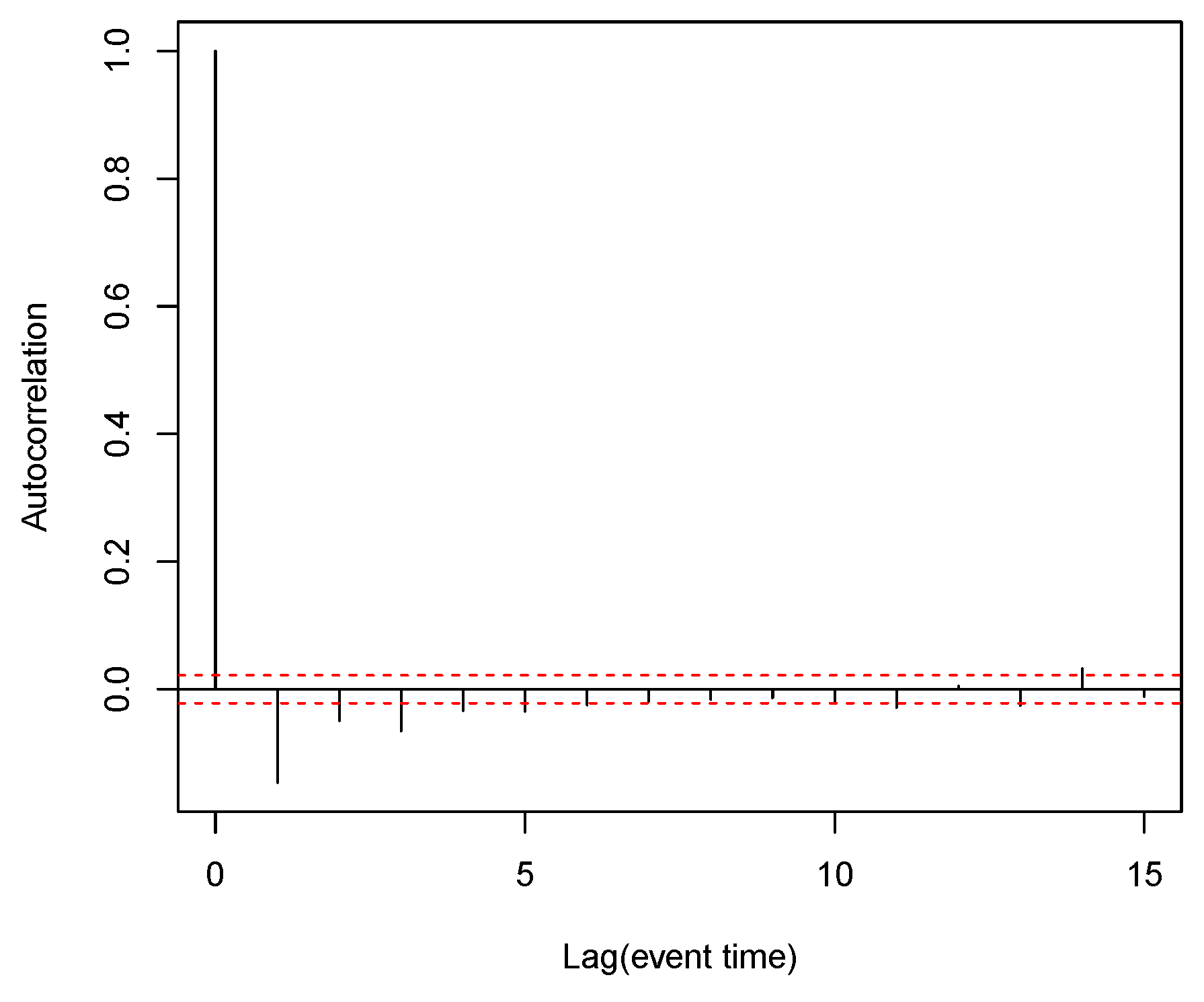
The simulation results demonstrate that our model also accurately captures realistic characteristics of the (steady-state) average behavior of the order book (OB) profile. Notably, the model successfully replicates the negative autocorrelation of price changes at the first lag. Empirical observations indicate that there is a pronounced negative autocorrelation at the first lag in the autocorrelation function of the transaction price returns. This negative autocorrelation is significant at the first lag and rapidly diminishes thereafter, as depicted in Figure 11.

Figure 11. Autocorrelation function of price return based on our simulations of the order book. The red dashed line represents the 95% confidence interval. Figure created by H.Rojas.

This phenomenon is commonly referred to as the bid–ask bounce [12], largely arising from having distinct trading prices for buyer-initiated and seller-initiated transactions. While this negative autocorrelation vanishes when considering aggregate returns, it is a noteworthy microstructural effect that must be considered in an order book model. Our model successfully replicates this empirical characteristic. Therefore, we conclude that we have sufficient evidence to argue that our model reproduces qualitative characteristics that are realistic and relevant.

4.4. Application: Prediction of Next Price Jump Direction

In this section, we present a direct application of our model that corresponds to the short-term forecast of price movement; that is, we use the proposed model to calculate the probability that the price will increase in the next jump, this probability is conditional on the observed state of the OB. This amount is particularly important in financial trading as it is used in the design of high-frequency trading strategies. From the transition rates of the price process $X\left(t\right)$ in (4), the probability that the price will increase in the next jump conditional to the observed state of the OB is given by

$$p(b,a):=\mathbb{P}\left\{\Delta P>0\left|X\right(t)=(b,a)\right\}=\left\{\begin{array}{cc}\frac{{\alpha }_{+}}{{\alpha }_{+}+{\beta }_{-}},& \mathrm{if}a-b=1,\hfill \\ & \\ \frac{{\alpha }_{+}+{\beta }_{+}}{{\gamma }_{+}+{\gamma }_{-}},& \mathrm{if}a-b>1,\hfill \end{array}\right.$$

(11)

where $\Delta P$ is the change in the mid-price. To increase the precision of the forecasts, we suggest calculating the theoretical probabilities $p(b,a)$ taking into account the different fixed values of the imbalance and the spread, that is,

$$\mathrm{Imbalance}=\frac{V\left(a\right)}{V\left(a\right)+V\left(b\right)}\mathrm{and}\mathrm{Spread}=a-b,$$

where $V\left(a\right)$ is the numbers of ask orders and $V\left(b\right)$ the numbers of bid orders. In other words, we will use (11) for buckets or bins generated by combinations of spread bid–ask and imbalance values.

As for the calculation of the IV, for the purposes of empirical contrast of the theoretical quantities $p(b,a)$, the observed variations in the mid-price were classified into two categories. Variations with mid-price increases were categorized as up variations. On the other hand, downward variations were categorized as down variations. Once the variations in mid-prices were dichotomized, the total set of 305 thousand observations was divided into two sub-samples.

The first sub-sample, which we call the training sample, corresponded to 70% of the total observations and was used to estimate the model parameters. The second sub-sample, called the test sample, corresponding to 30% of the total observations, was used to validate the performance of the model forecasts.

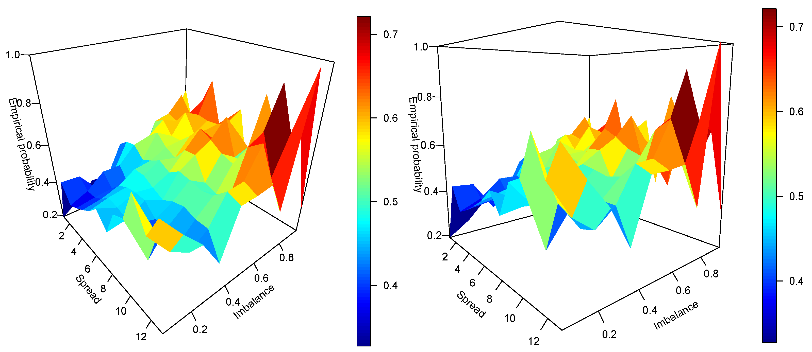
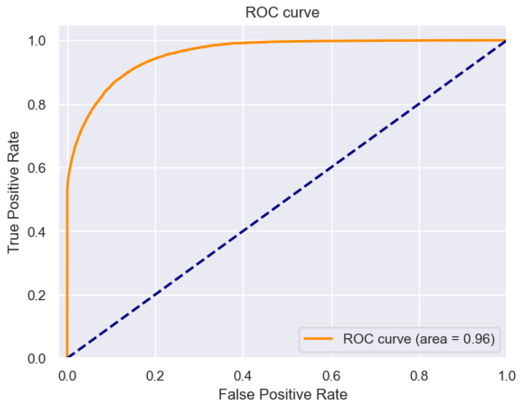
With the estimated parameters, we calculate the empirical probabilities $\widehat{p}(b,a)$ using the test sample. Additionally, using the (11), we calculate the theoretical predicted probabilities $p(b,a)$ for the same dataset. For comparison purposes, in Figure 12, we present the results for both quantities. The figure confirms the good precision of the model to predict variations in the mid-price. Furthermore, to numerically confirm the precision of our forecasts, we present in Figure 13 the ROC curve, which corroborates, with a score of 96%, the predictive power of the model to events of up variations in the mid-price.

Figure 12. Empirical probabilities $\widehat{p}(b,a)$ versus theoretical probabilities $p(b,a)$. Figures created by H.Rojas.

Figure 13. Accuracy in classifying variations up; the event of interest (target variable) is the variation up. Figure created by H.Rojas.

5. Discussion: Other Regimes

In this section, we outline the formulations for the remaining two regimes that can be encompassed within our general model. As previously indicated, the primary findings of this article have the potential for generalization to these alternative regimes. However, our belief is that, in qualitative terms, there will be minimal disparities between the outcomes. We anticipate that these subsequent formulations will serve as incentives for future research endeavors aimed at extending and broadening the scope of our results.

5.1. Almost Uniform Catastrophes

As we mentioned before, the large deviations were proved for the so-called almost uniform catastrophes. Recall that in order to close the spread of length k (with probability $\frac{{\gamma }_{-}}{\gamma }$), we choose the next state for the spread with the same probability (uniformly) from the set $I_k=\{1,\cdots ,k-1\}$ and denote these probabilities as $Q_i\left(k\right),i\in I_k$, and here $Q_i\left(k\right)=\frac{1}{k-1}$. The almost uniform distribution is defined by the following form of probabilities $Q_i\left(k\right),1\le i\le k-1$: there exists a constant $c>1$ such that for all $k\in \mathbb{N}$

$$\frac{1}{c(k-1)}\le Q_i\left(k\right)\le \frac{c}{k-1},$$

for all $i\in I_k$. It extends the class of models for highly competitive regimes. For example, for any length k of the spread, it can be divided into some parts, say two parts, and we say that with probability $0.7$, we choose one part, and then uniformly the state from this part is chosen; with probability $0.3$, the second part is chosen and the corresponding state is chosen uniformly.

All the proofs above can be slightly modified.

5.2. Non-Competitive Regime

The main features of the non-competitive regime (NC regime) are small openings of the spread, similar to the HC regime. However, in the NC regime, there is a slow decrease (following a power law) in the spread. This slow decrease occurs because agents placing limit orders within the spread prioritize achieving an optimal price in their quotes. Compared to the HC regime the agents are less impatient. With some constant rate, the spread opens by one tick. For the closing spread, let $k>1$ be the spread size, and the variation in the prices $\Delta$ is chosen from $I_k=\{1,\cdots ,k-1\}$ according to the rate which is proportional to ${\Delta }^{-\mu }$, where $\mu$ is a fixed positive number. The parameter $\mu$ can be interpreted as a behavioral measure for agents to obtain a more favorable price in their negotiations.

Model: Closing the Spread Polynomially

In order to define the rates for the NC regime, let us again fix parameters ${\alpha }_{+}^c,{\alpha }_{-}^c,{\beta }_{+}^c,{\beta }_{-}^c,$ which are strictly positive real numbers. Suppose that at some moment the chain is at some state $(b,a)\in \mathbb{X}$, then the transition rates for the Markov chain $X\left(t\right)$ in this regime are defined in the following way:

$$\begin{array}{c}\hfill {\alpha }_{+}(\Delta )=\left\{\begin{array}{cc}\hfill {\alpha }_{+}^c,& \mathrm{if} \Delta =1;\hfill \\ \hfill 0,& \mathrm{otherwise};\hfill \end{array}\right.{\alpha }_{-}(\Delta )=\left\{\begin{array}{cc}\hfill \frac{{\alpha }_{-}^c}{{\Delta }^{\mu }},& \mathrm{if} a-b>1 \mathrm{for} \mathrm{any} \Delta \in I_{a-b};\hfill \\ \hfill 0,& \mathrm{otherwise};\hfill \end{array}\right.\\ \hfill {\beta }_{-}(\Delta )=\left\{\begin{array}{cc}\hfill {\beta }_{-}^c,& \mathrm{if} \Delta =1;\hfill \\ \hfill 0,& \mathrm{otherwise};\hfill \end{array}\right.{\beta }_{+}(\Delta )=\left\{\begin{array}{cc}\hfill \frac{{\beta }_{+}^c}{{\Delta }^{\mu }},& \mathrm{if} a-b>1 \mathrm{for} \mathrm{any} \Delta \in I_{a-b};\hfill \\ \hfill 0,& \mathrm{otherwise}.\hfill \end{array}\right.\end{array}$$

(12)

For illustration, see Figure 14 in the case when $a-b=3$.

Figure 14. The rates for the non-competitive model. An illustrative example for the case when $a-b=3$. Figure created by A.Yambartsev.

Again, as before, first, we study the Markov chain $S\left(t\right)$. Suppose that at some moment t the chain is at some state $k\in \mathbb{N}$, and let ${\gamma }_{+}^c:={\beta }_{-}^c+{\alpha }_{+}^c$ and ${\gamma }_{-}^c:={\beta }_{+}^c+{\alpha }_{-}^c$, then

$$\begin{array}{cccc}\hfill k& \to k+1\hfill & \hfill \mathrm{with} \mathrm{rate}& {\gamma }_{+}^c,\hfill \\ \hfill k& \to k-\Delta \hfill & \hfill \mathrm{with} \mathrm{rate}& \frac{{\gamma }_{-}^c}{{\Delta }^{\mu }} \mathrm{for} \Delta \in I_k.\hfill \end{array}$$

(13)

These transitions suggest that the spread dynamics have a slow reversal process to their typical values, this is because each liquidity provider competes with the others to spread closing.

5.3. Low Liquidity with Gaps Regime

The main feature of low liquidity with gaps regime (LLG regime) is that the spread can open by more than one tick, this is due to the existence of gaps in the OB. The spread decreases similarly to the NC regime.

Model

Let us fix parameters ${\alpha }_{+}^l,{\alpha }_{-}^l,{\beta }_{+}^l,{\beta }_{-}^l,{\kappa }_a,{\kappa }_b$ and $\theta \in (0,1)$, which are strictly positive real numbers. Suppose that at some moment the chain is at some state $(b,a)\in \mathbb{X}$, then the transition rates for the Markov chain $X\left(t\right)$ for this regime are defined as follows.

$$\begin{array}{cc}\hfill {\alpha }_{+}(\Delta )& =\left\{\begin{array}{cc}\frac{{\alpha }_{+}^l}{{(a-b)}^{{\kappa }_a}}·\theta {(1-\theta )}^{\Delta -1},& \mathrm{for} \Delta \in \mathbb{N};\hfill \\ 0,& \mathrm{otherwise};\hfill \end{array}\right.\hfill \\ \hfill {\alpha }_{-}(\Delta )& =\left\{\begin{array}{cc}\frac{{\alpha }_{-}^l}{{(a-b)}^{{\kappa }_a}}·\frac{\theta {(1-\theta )}^{\Delta -1}}{1-{(1-\theta )}^{a-b-1}},& \mathrm{if} a-b>1\mathrm{for} \Delta \in I_{a-b};\hfill \\ 0,& \mathrm{otherwise};\hfill \end{array}\right.\hfill \\ \hfill {\beta }_{-}(\Delta )& =\left\{\begin{array}{cc}\frac{{\beta }_{-}^l}{{(a-b)}^{{\kappa }_b}}·\theta {(1-\theta )}^{\Delta -1},& \mathrm{for} \Delta \in \mathbb{N};\hfill \\ 0,& \mathrm{otherwise};\hfill \end{array}\right.\hfill \\ \hfill {\beta }_{+}(\Delta )& =\left\{\begin{array}{cc}\frac{{\beta }_{-}^l}{{(a-b)}^{{\kappa }_b}}·\frac{\theta {(1-\theta )}^{\Delta -1}}{1-{(1-\theta )}^{a-b-1}},& \mathrm{if} a-b>1\mathrm{for} \Delta \in I_{a-b};\hfill \\ 0,& \mathrm{otherwise}.\hfill \end{array}\right.\hfill \end{array}$$

(14)

For illustration, see Figure 15 in the case when $a-b=3$.

Figure 15. The rates for the low-liquidity model. An illustrative example for the case when $a-b=3$. Figure created by A.Yambartsev.

This Markov chain can be described more easily informally in the following way: for a given state $(b,a)$

• with the rate $\frac{{\alpha }_{+}^l}{{(a-b)}^{{\kappa }_a}}$, the chain decides to increase the ask price, and it chooses the increment according to the geometric distribution with parameter $\theta$;
• with the rate $\frac{{\alpha }_{-}^l}{{(a-b)}^{{\kappa }_a}}$, the chain decides to decrease the ask price, and it chooses the increment according to the truncated geometric distribution with parameter $\theta$ and values $I_{a-b}=\{1,\cdots ,a-b-1\}$;
• with the rate $\frac{{\beta }_{-}^l}{{(a-b)}^{{\kappa }_b}}$, the chain decides to decrease the bid price, and it chooses the increment according to the geometric distribution with parameter $\theta$;
• with the rate $\frac{{\beta }_{+}^l}{{(a-b)}^{{\kappa }_b}}$, the chain decides to increase the bid price, and it chooses the increment according to the truncated geometric distribution with parameter $\theta$ and values $I_{a-b}=\{1,\cdots ,a-b-1\}$.

Once more, following the same approach, we initiate our analysis by studying the Markov chain $S\left(t\right)$. Let us consider a particular time instance t when the chain is situated at state $k\in \mathbb{N}$, then the following transitions occur:

$$\begin{array}{cccc}\hfill k& \to k+\Delta \hfill & \hfill \mathrm{with} \mathrm{rate}& \left(\frac{{\alpha }_{+}^l}{k^{{\kappa }_a}}+\frac{{\beta }_{-}^l}{k^{{\kappa }_b}}\right)·\theta {(1-\theta )}^{\Delta -1}, \mathrm{for} \Delta \in \mathbb{N},\hfill \\ \hfill k& \to k-\Delta \hfill & \hfill \mathrm{with} \mathrm{rate}& \left(\frac{{\alpha }_{-}^l}{k^{{\kappa }_a}}+\frac{{\beta }_{+}^l}{k^{{\kappa }_b}}\right)·\frac{\theta {(1-\theta )}^{\Delta -1}}{1-{(1-\theta )}^{k-1}}, \mathrm{for} \Delta \in I_k.\hfill \end{array}$$

(15)

6. Conclusions

We propose a straightforward model for price dynamics in an OB with liquidity fluctuations. Unlike [9], our model does not explicitly capture liquidity fluctuations but still offers a reasonable approximation for empirical observations. The continuous-time Markov process describing spread dynamics falls into the category of Poisson processes with uniform catastrophes, where the eliminated fraction of the population follows a uniform distribution. Large deviation results for such processes have been studied in [15,16].

When the spread closure (catastrophe) follows a uniform distribution, it accurately represents a scenario of complete uncertainty in the decisions of bidders. In such a case, any change in the spread is equally probable, indicating an exceptionally unusual situation often associated with extremely high volatility. By examining such scenarios, it is conceivable, to a significant extent, to devise a decision-making algorithm with a substantial degree of reliability. Alternatively, if one seeks to hedge against substantial fluctuations in the spread, our model may offer insights into calculating the appropriate insurance premiums needed to ensure that the risk of financial collapse remains below a predetermined threshold.

We examined the asymptotic behavior of the model, which involved determining the invariant measure (a rare case where it can be derived explicitly), and establishing results such as the law of large numbers, the central limit theorem, and large deviations. These theoretical findings were utilized in Monte Carlo simulations to validate that our model reproduces relevant empirical characteristics.

We conclude our paper by discussing potential future research directions, including the exploration of other liquidity regimes and model extensions for various applications.

Appendix A.1. Ergodicity and Invariant Measure for S(t): Proof of Theorem 1

To establish positive recurrence, we introduce a Lyapunov function based on the criteria for continuous-time Markov chains as outlined in [18], Theorem 1.7. Positive recurrence can be inferred from the existence of a non-negative function f (Lyapunov function) across the set of states, a small positive value $\epsilon$, and a finite set of states F. Specifically, by applying the process generator $\Gamma$ to function f, we ensure that $\Gamma f\left(x\right)<-\epsilon$ holds true for all states x not within the set F.

Recall that the generator $\Gamma$ for a discrete-state Markov process is represented by the matrix $\Gamma =\left({\Gamma }_{xy}\right)$, where ${\Gamma }_{xy}$ for $x\ne y$ corresponds to the transition rate from state x to state y, and ${\Gamma }_{xx}=-{\sum }_{y\ne x}{\Gamma }_{xy}$. Applying the generator for the identity function $f\left(x\right)=x$, we obtain

$$\Gamma f\left(k\right)={\gamma }_{+}(k+1)+\sum _{x\in I_k}\frac{{\gamma }_{+}}{k-1}x-({\gamma }_{+}+{\gamma }_{-})k={\gamma }_{+}-\frac{{\gamma }_{-}k}{2}<-1,$$

for all $k:k>2({\gamma }_{+}+1)/{\gamma }_{-}$. The last inequality provides the finite set $F=\{k\le 2({\gamma }_{+}+1)/{\gamma }_{-}\}$ for the criteria above with $\epsilon =1$. Thus, the criterion ensures that the Markov process is positively recurrent.

The formula for the invariant measure can be verified through direct examination using the global balance equations. Beginning with the system of global balance equations, we derive the following.

$$\left\{\begin{array}{cc}\hfill {\gamma }_{+}\mu \left(1\right)& ={\gamma }_{-}\mu \left(2\right)+\frac{{\gamma }_{-}}{2}\mu \left(3\right)+\frac{{\gamma }_{-}}{3}\mu \left(4\right)+\cdots \hfill \\ \hfill ({\gamma }_{+}+{\gamma }_{-})\mu \left(2\right)& ={\gamma }_{+}\mu \left(1\right)+\frac{{\gamma }_{-}}{2}\mu \left(3\right)+\frac{{\gamma }_{-}}{3}\mu \left(4\right)+\cdots \hfill \\ \hfill ({\gamma }_{+}+{\gamma }_{-})\mu \left(3\right)& ={\gamma }_{+}\mu \left(2\right)+\frac{{\gamma }_{-}}{3}\mu \left(4\right)+\frac{{\gamma }_{-}}{4}\mu \left(5\right)+\cdots \hfill \\ \hfill \cdots \\ \hfill ({\gamma }_{+}+{\gamma }_{-})\mu \left(n\right)& ={\gamma }_{+}\mu (n-1)+\frac{{\gamma }_{-}}{n}\mu (n+1)+\cdots \hfill \\ \hfill \cdots \end{array}\right.\iff \left\{\begin{array}{cc}\hfill 2{\gamma }_{+}\mu \left(1\right)& =({\gamma }_{+}+2{\gamma }_{-})\mu \left(2\right)\hfill \\ \hfill (2{\gamma }_{+}+{\gamma }_{-})\mu \left(2\right)& ={\gamma }_{+}\mu \left(1\right)+({\gamma }_{+}+{\gamma }_{-}+\frac{{\gamma }_{-}}{2})\mu \left(3\right)\hfill \\ \hfill (2{\gamma }_{+}+{\gamma }_{-})\mu \left(3\right)& ={\gamma }_{+}\mu \left(2\right)+({\gamma }_{+}+{\gamma }_{-}+\frac{{\gamma }_{-}}{3})\mu \left(4\right)\hfill \\ \hfill \cdots \\ \hfill (2{\gamma }_{+}+{\gamma }_{-})\mu \left(n\right)& ={\gamma }_{+}\mu (n-1)+({\gamma }_{+}+{\gamma }_{-}+\frac{{\gamma }_{-}}{n})\mu (n+1)\hfill \\ \hfill \cdots \end{array}\right.$$

Dividing the left side and right side on ${\gamma }_{+}+{\gamma }_{-}$ and using the notation $p:=\frac{{\gamma }_{+}}{{\gamma }_{+}+{\gamma }_{-}},$$q:=1-p$, we rewrite the last system as

$$\left\{\begin{array}{cc}\hfill \mu \left(2\right)& =\frac{2p}{1+q}\mu \left(1\right)\hfill \\ \hfill \mu \left(3\right)& =\frac{1+p}{1+\frac{q}{2}}\mu \left(2\right)-\frac{p}{1+\frac{q}{2}}\mu \left(1\right)\hfill \\ \hfill \cdots \\ \hfill \mu \left(n\right)& =\frac{1+p}{1+\frac{q}{n-1}}\mu (n-1)-\frac{p}{1+\frac{q}{n-1}}\mu (n-2)\hfill \\ \hfill \cdots \end{array}\right.\iff \left\{\begin{array}{cc}\hfill \mu \left(2\right)& =\frac{2p}{1+q}\mu \left(1\right)\hfill \\ \hfill \mu \left(3\right)& =\frac{3p^2}{(1+q)(1+\frac{q}{2})}\mu \left(1\right)\hfill \\ \hfill \cdots \\ \hfill \mu \left(n\right)& =\frac{n{p}^{n-1}}{{\prod }_{i=1}^{n-1}(1+\frac{q}{i})}\mu \left(1\right)\hfill \\ \hfill \cdots \end{array}\right.$$

After the normalizing of the relation

$$\mu \left(n\right)=\frac{n{p}^{n-1}}{{\prod }_{i=1}^{n-1}(1+\frac{q}{i})}\mu \left(1\right)$$

(A1)

and since $\mu$ is the probability measure, $\sum \mu \left(k\right)=1$, we return the notation ${\gamma }_{\pm }$ and obtain Formula (6).

Appendix A.2. Law of Large Numbers: Proof of Theorem 2

Perhaps the most straightforward method to prove the LLN involves the ergodic theorem for discrete-time Markov chains. Let $s_n$ denote the embedded discrete-time Markov chain on $\mathbb{N}$ derived from $S(·)$, with the following transition probabilities:

$$p(k,l):=\mathbb{P}(s_{n+1}=l\mid s_n=k)=\left\{\begin{array}{cc}\hfill 1,& \mathrm{if} l=2 \mathrm{and} k=1,\hfill \\ \hfill \frac{{\gamma }_{+}}{{\gamma }_{+}+{\gamma }_{-}},& \mathrm{if} l=k+1, \mathrm{when} k>1,\hfill \\ \hfill \frac{{\gamma }_{-}}{{\gamma }_{+}+{\gamma }_{-}}\frac{1}{k-1},& \mathrm{if} l\in I_k \mathrm{and} k>1.\hfill \end{array}\right.$$

Consider the stationary measure $\pi =\left(\pi \right(s),s\in \mathbb{N})$ associated with the chain $s_n$. Evidently, the relation (6) for the stationary measure $\mu$ can be transformed into the following relation for the stationary measure $\pi$:

$$\pi \left(n\right)=\frac{n{p}^{n-2}}{{\prod }_{i=1}^{n-1}(1+\frac{q}{i})}\pi \left(1\right),n\ge 2.$$

(A2)

This transformation can be verified directly using the global balance equations of the discrete-time Markov chain $s_n$.

Denote as $p_n$ the discrete-time embedding chain corresponding to the continuous-time bid-price process $P_b\left(t\right)$. The behavior of $p_n$ can be expressed as a function of the spread dynamics $s_n$ using the following formula.

$$p_n=\sum _{i=0}^{n}F(s_{n-1},s_n,U_n),$$

(A3)

where

$$U_n=(U_n^1,U_n^2)$$

is the sequence of independent and identically distributed random vectors such that

$$\mathbb{P}((U_n^1,U_n^2)=(1,0))=\frac{{\beta }_{-}}{{\gamma }_{+}}\left(1-\frac{{\beta }_{+}}{{\gamma }_{-}}\right),\mathbb{P}((U_n^1,U_n^2)=(1,1))=\frac{{\beta }_{-}}{{\gamma }_{+}}\frac{{\beta }_{+}}{{\gamma }_{-}},$$

$$\mathbb{P}((U_n^1,U_n^2)=(0,0))=\left(1-\frac{{\beta }_{-}}{{\gamma }_{+}}\right)\left(1-\frac{{\beta }_{+}}{{\gamma }_{-}}\right),\mathbb{P}((U_n^1,U_n^2)=(0,1))=\left(1-\frac{{\beta }_{-}}{{\gamma }_{+}}\right)\frac{{\beta }_{+}}{{\gamma }_{-}},$$

and where the function F is

$$F(s_{n-1},s_n,U_n)=\left\{\begin{array}{cc}\hfill -1,& \mathrm{if} s_n=s_{n-1}+1 \mathrm{and} U_n^1=1;\hfill \\ \hfill s_{n-1}-s_n,& \mathrm{if} s_n<s_{n-1} \mathrm{and} U_n^2=1;\hfill \\ \hfill 0,& \mathrm{otherwise}.\hfill \end{array}\right.$$

(A4)

Note that

$${\widehat{s}}_n:=(s_{n-1},s_n,U_n)$$

(A5)

is a Markov chain, and let $\widehat{\pi }$ be its invariant measure. Observe that the discrete part of the invariant measure $\widehat{\pi }$ for the process $(s_{n-1},s_n)$ is the product $\widehat{\pi }(x,y)=\pi \left(x\right)p(x,y)$. By the ergodic theorem, we obtain the LLN for the embedding chain $p_n$.

Lemma A1.

$$\frac{p_n}{n}\to va.s.n\to \infty$$

(A6)

where

$$v=-\frac{{\beta }_{-}}{{\gamma }_{+}+{\gamma }_{-}}-\frac{\pi \left(1\right)}{{\gamma }_{+}+{\gamma }_{-}}\left(\frac{{\beta }_{-}{\gamma }_{-}}{{\gamma }_{+}}+\frac{{\beta }_{+}}{2}\right)+\frac{{\beta }_{+}}{{\gamma }_{+}+{\gamma }_{-}}\frac{1}{2}\sum _{s=1}^{\infty }s\pi \left(s\right).$$

Proof. 

The ergodic theorem states the convergence (A6). Thus, we need only to find the v, which is the expectation over the invariant measure $\widehat{\pi }$ of the increments $F\left({\widehat{s}}_n\right)$:

$$\begin{array}{cc}\hfill {\mathbb{E}}_{\widehat{\pi }}\left(F\left({\widehat{s}}_n\right)\right)=& -\pi \left(1\right)\frac{{\beta }_{-}}{{\gamma }_{+}}-\sum _{s=2}^{\infty }\pi \left(s\right)\frac{{\gamma }_{+}}{{\gamma }_{+}+{\gamma }_{-}}\frac{{\beta }_{-}}{{\gamma }_{+}}+\sum _{s_2=2}^{\infty }\sum _{s_1=1}^{s_2-1}(s_2-s_1)\pi \left(s_2\right)\frac{{\gamma }_{-}}{{\gamma }_{+}+{\gamma }_{-}}\frac{1}{s_2-1}\frac{{\beta }_{+}}{{\gamma }_{-}}\hfill \\ \hfill =& -\frac{{\beta }_{-}}{{\gamma }_{+}+{\gamma }_{-}}-\frac{\pi \left(1\right)}{{\gamma }_{+}+{\gamma }_{-}}\left(\frac{{\beta }_{-}{\gamma }_{-}}{{\gamma }_{+}}+\frac{{\beta }_{+}}{2}\right)+\frac{{\beta }_{+}}{{\gamma }_{+}+{\gamma }_{-}}\frac{1}{2}\sum _{s=1}^{\infty }s\pi \left(s\right),\hfill \end{array}$$

which finishes the proof of the lemma. □

To finish the proof of Theorem 2, we observe

$$\begin{array}{cc}\hfill \underset{t\to \infty }{lim}\frac{P_b\left(t\right)}{t}& =\underset{t\to \infty }{lim}\frac{p_{N_t}}{N_t}\frac{N_t}{t}=v({\gamma }_{+}+{\gamma }_{-})\hfill \\ & =-{\beta }_{-}-\pi \left(1\right)\left(\frac{{\beta }_{-}{\gamma }_{-}}{{\gamma }_{+}}+\frac{{\beta }_{+}}{2}\right)+\frac{{\beta }_{+}}{2}\sum _{s=1}^{\infty }s\pi \left(s\right)=:D,\hfill \end{array}$$

where $N_t$ is the Poisson process with rate ${\gamma }_{+}+{\gamma }_{-}$.

Appendix A.3. CLT for Embedding p_n: Proof of Lemma 1

For instance, one approach to proving this is by demonstrating the geometric ergodicity of the chain ${\widehat{s}}_n$, which indicates a geometric rate of convergence to the invariant measure:

$$\parallel P^n(x,·)-\widehat{\pi }(·)\parallel \le M\left(x\right)q^n, \mathrm{for} \mathrm{some} q<1,$$

(A7)

where $\parallel ·\parallel$ stands for the total variation norm. Subsequently, we can apply the results applicable to geometrically ergodic chains. Formally, this necessitates establishing that the chain ${\widehat{s}}_n$, defined by (A5), is a Harris ergodic Markov chain, which indeed holds true for ${\widehat{s}}_n$. For further details, please refer to [19].

Theorem A1

(Corollary 2, [19]). Let X be a Harris ergodic Markov chain on $\mathbb{X}$ with invariant distribution π and let $f:\mathbb{X}\to \mathbb{R}$ be a Borel function. Assume that X is geometrically ergodic and ${\mathbb{E}}_{\pi }{\left|f\left(x\right)\right|}^{2+\delta }<\infty$ for some $\delta >0$. Then, for any initial distribution, as $n\to \infty$

$$\sqrt{n}({\overline{f}}_n-{\mathbb{E}}_{\pi }f)\to N(0,{\sigma }_f^2)$$

in distribution.

Let us begin by proving the geometric ergodicity of the chain ${\widehat{s}}_n$. General results exist concerning the so-called drift conditions for establishing geometric ergodicity in chains, as detailed in [20]. However, for countable Markov chains, we can utilize the criteria outlined in [21] (refer to Theorem 2):

A countable Markov chain is geometrically ergodic if there exists a finite set $B\subset \mathbb{X}$ and function $g\left(x\right)\ge 0$, $x\in \mathbb{X}$ such that ${\mathbb{E}}_x{e}^{g\left(X_1\right)-g\left(X_0\right)}\le q<1,$ when $x\notin B$ and ${\mathbb{E}}_x{e}^{g\left(X_1\right)-g\left(X_0\right)}<\infty$, if $x\in B$.

Proof. 

Utilizing the criteria, let $V(·)\equiv e^{g(·)}$. To check the conditions we consider the function $V(·)$ for the chain ${\widehat{s}}_n$, defined as follows:

$$V(i,j,u)=e^{ln(i^2+j^2)}=i^2+j^2.$$

For simplicity, let us assume $p_{+}=\frac{{\gamma }_{+}}{{\gamma }_{+}+{\gamma }_{-}}$ and $p_{-}=\frac{{\gamma }_{-}}{{\gamma }_{+}+{\gamma }_{-}}$. Then,

$$\begin{array}{ccc}\hfill \mathbb{E}\left.\left(\frac{V(s_n,s_{n+1},U_{n+1})}{V(s_{n-1},s_n,U_n)}\right|s_{n-1}=y,s_n=x\right)& =& \sum _{k=1}^{x-1}\left(\frac{{(x-k)}^2+x^2}{x^2+y^2}\right)\frac{p_{-}}{x-1}+\left(\frac{{(x+1)}^2+x^2}{y^2+x^2}\right)p_{+}\hfill \\ & =& \frac{x(2x-1)}{6(x^2+y^2)}{p}_{-}+\frac{x^2}{x^2+y^2}{p}_{-}+\frac{{(x+1)}^2+x^2}{y^2+x^2}{p}_{+}.\hfill \end{array}$$

(A8)

Consider two cases. First, we suppose that $x<y$. Then,

$$\left(\mathrm{A}8\right)\le \frac{x(2x-1)}{6(x^2+{(x+1)}^2)}{p}_{-}+\frac{x^2}{x^2+{(x+1)}^2}{p}_{-}+\frac{{(x+1)}^2+x^2}{x^2+{(x+1)}^2}{p}_{+}<\frac{2}{3}{p}_{-}+p_{+}\le q<1.$$

Thus, the condition holds for all $(x,y)$ such that $x<y$. In the second case, $x>y$, we have $y=x-1$:

$$\begin{array}{ccc}\hfill \left(\mathrm{A}8\right)& =& \frac{x(2x-1)}{6(x^2+{(x-1)}^2)}{p}_{-}+\frac{x^2}{x^2+{(x-1)}^2}{p}_{-}+\frac{{(x+1)}^2+x^2}{x^2+{(x-1)}^2}{p}_{+}\hfill \\ & =& \frac{(8x^2-x)p_{-}+24x{p}_{+}}{6(x^2+{(x-1)}^2)}+p_{+}.\hfill \end{array}$$

There is no $q<1$ such that (A8) $\le q$ for all x. But it is easy to see that there exists $q>\frac{2}{3}{p}_{-}+p_{+}$ and $C\equiv C(p_{-},p_{+},q)>0$ such that for all $(x,y)$ under the condition $x\ge C$

$$\left(\mathrm{A}8\right)\le q<1.$$

It is easy to see that

$$\underset{x}{sup}\frac{(8x^2-x)p_{-}+24x{p}_{+}}{6(x^2+{(x-1)}^2)}+p_{+}<\infty .$$

Thus, in this case, we can define the finite set B from the condition as

$$B=\left\{(x,y):x\le C,y\le x,U_n\in \{(0,0),(0,1),(1,0),(1,1)\}\right\}.$$

This completes the proof of the geometrical ergodicity of the chain ${\widehat{s}}_n$. □

For the second condition of the CLT theorem, it is necessary to verify that $E_{\widehat{\pi }}{\left|F\left({\widehat{s}}_n\right)\right|}^{2+\delta }<\infty$ for a certain $\delta >0$, where the function F is defined by (A4). To achieve this, we require insights into the behavior of the invariant measure.

Proof. 

As before, let $\pi$ be the invariant measure for the chain $s_n$. The condition takes the following form:

$$\begin{array}{cc}\hfill {\mathbb{E}}_{\widehat{\pi }}{\left|F\left({\widehat{s}}_n\right)\right|}^{2+\delta }& =\sum _{x=1}^{\infty }\left(\sum _{k=1}^{x-1}{k}^{2+\delta }\widehat{\pi }(x,x-k)\frac{{\beta }_{+}}{{\gamma }_{-}}+\widehat{\pi }(x,x+1)\frac{{\beta }_{-}}{{\gamma }_{+}}\right)\hfill \\ \hfill & =\frac{{\beta }_{-}}{{\gamma }_{+}+{\gamma }_{-}}+\frac{{\beta }_{+}}{{\gamma }_{+}+{\gamma }_{-}}\sum _{x=1}^{\infty }\pi \left(x\right)\sum _{k=2}^{x-1}\frac{k^{2+\delta }}{x-1}\hfill \\ \hfill & <\frac{{\beta }_{-}}{{\gamma }_{+}+{\gamma }_{-}}+\frac{{\beta }_{+}}{{\gamma }_{+}+{\gamma }_{-}}\frac{1}{3+\delta }\sum _{x=1}^{\infty }\pi \left(x\right)\frac{x^{3+\delta }}{x-1}.\hfill \end{array}$$

(A9)

Thus, if we prove that $\pi \left(x\right)$ decreases sufficiently fast, then the last series in (A9) will converge. Indeed, from the relation (A2) we obtain immediately

$$\pi \left(n\right)<n{p}^{n-2}\pi \left(1\right),$$

which provides the convergence of the last series in (A9). This establishes the conditions for the central limit theorem (CLT). □

With that, we conclude the proof of the CLT, as stated in Lemma 1.

Appendix A.4. CLT for Continuous-Time P b (t): Proof of Theorem 3

Based on the result above, let us proceed to establish the central limit theorem for the price process $P_b\left(t\right)$. As previously mentioned, consider $N_t$ to be the Poisson process with rate $\gamma ={\gamma }_{+}+{\gamma }_{-}$, representing the count of jumps for the process $X\left(t\right)=\left(P_b\left(t\right),P_a\left(t\right)\right)$. The subsequent representation holds:

$$\begin{array}{c}\hfill \sqrt{t}\left(\frac{P_b\left(t\right)}{t}-D\right)=\sqrt{N_t}\left(\frac{p_{N_t}}{N_t}-v\right)\sqrt{\frac{N_t}{t}}+\sqrt{t}\left(\frac{N_t}{t}v-D\right)\end{array}$$

According to Lemma 1 and CLT for the Poisson process, we expect that as $t\to \infty$

$$\begin{array}{cc}\hfill \sqrt{N_t}\left(\frac{p_{N_t}}{N_t}-v\right)& \to N(0,{\sigma }^2) \mathrm{in} \mathrm{distribution} \mathrm{for} \mathrm{some} {\sigma }^2\hfill \\ \hfill \sqrt{t}\left(\frac{N_t}{t}-\gamma \right)& \to N(0,\gamma ) \mathrm{in} \mathrm{distribution} \hfill \\ \hfill \frac{N_t}{t}& \to \gamma a.s.\hfill \end{array}$$

(A10)

The second and third convergence are well known when the first one can be proved as follows: let $F_n\left(x\right)$ be the cumulative distribution function of the scaled embedded price Markov chain $p_n$ from Lemma 1, then for any $\delta >0$ there exists $n_{\delta }$ such that for all $n>n_{\delta }$

$$\left|F_n\left(x\right)-{\Phi }_{{\sigma }^2}\left(x\right)\right|<\delta ,$$

where ${\Phi }_{{\sigma }^2}\left(x\right)$ stands for the cumulative normal distribution with zero mean and variance ${\sigma }^2$. Then,

$$\begin{array}{cc}\hfill \mathbb{P}\left(\sqrt{N_t}\left(\frac{p_{N_t}}{N_t}-v\right)\le x\right)& =\mathbb{P}\left.\left(\sqrt{N_t}\left(\frac{p_{N_t}}{N_t}-v\right)\le x\right|N_t\le n_{\delta }\right)\mathbb{P}(N_t\le n_{\delta })\hfill \\ & +\sum _{n=n_{\delta }+1}^{\infty }\mathbb{P}\left.\left(\sqrt{N_t}\left(\frac{p_{N_t}}{N_t}-v\right)\le x\right|N_t=n\right)\mathbb{P}(N_t=n)\hfill \\ & \le \mathbb{P}(N_t\le n_{\delta })+{\Phi }_{{\sigma }^2}\left(x\right)+\delta \hfill \\ & \to {\Phi }_{{\sigma }^2}\left(x\right) \mathrm{as} t\to \infty , \mathrm{and} \mathrm{as} \delta \to 0\hfill \\ \hfill \mathbb{P}\left(\sqrt{N_t}\left(\frac{p_{N_t}}{N_t}-v\right)\le x\right)& \ge \left({\Phi }_{{\sigma }^2}\left(x\right)-\delta \right)\mathbb{P}(N_t>n_{\delta })\hfill \\ & ={\Phi }_{{\sigma }^2}\left(x\right)-\delta +\left({\Phi }_{{\sigma }^2}\left(x\right)-\delta \right)\mathbb{P}(N_t\le n_{\delta })\hfill \\ & \to {\Phi }_{{\sigma }^2}\left(x\right) \mathrm{as} t\to \infty , \mathrm{and} \mathrm{as} \delta \to 0.\hfill \end{array}$$

Observe that two normal variables from (A10) are not independent; however, they are asymptotically uncorrelated and, furthermore, asymptotically independent. To demonstrate this, consider variables

$$\sqrt{N_t}\left(\frac{p_{N_t}}{N_t}-v\right)\mathrm{and}\sqrt{t}\left(\frac{N_t}{t}-\gamma \right).$$

We will show that they are asymptotically independent.

Since the second variable is a measurable function of the $N_t$ it suffices to prove that for all $x\in \mathbb{R}$, all sets $A\subseteq \mathbb{N}$, and all $\epsilon >0$, the following inequality holds:

$$\underset{t\to \infty }{lim}\left|\mathbb{P}\left(\sqrt{N_t}\left(\frac{p_{N_t}}{N_t}-v\right)<x,N_t\in A\right)-{\Phi }_{{\sigma }^2}\left(x\right)\mathbb{P}(N_t\in A)\right|\le \epsilon .$$

(A11)

If the set A is bounded from above, then the inequality holds:

$$0\le \underset{t\to \infty }{lim}\mathbb{P}\left(\sqrt{N_t}\left(\frac{p_{N_t}}{N_t}-v\right)<x,N_t\in A\right)\le \underset{t\to \infty }{lim}\mathbb{P}(N_t\in A)=0.$$

Suppose now that A is not bounded. In this case, for any $\delta >0$ we obtain

$$\begin{array}{cc}& \underset{t\to \infty }{lim}\mathbb{P}\left(\sqrt{N_t}\left(\frac{p_{N_t}}{N_t}-v\right)<x,N_t\in A\right)\hfill \\ & =\underset{t\to \infty }{lim}\mathbb{P}\left(\sqrt{N_t}\left(\frac{p_{N_t}}{N_t}-v\right)<x,N_t\in A\cap [0,n_{\delta }]\right)+\underset{t\to \infty }{lim}\sum _{k=n_{\delta }+1}^{\infty }\mathbb{P}\left(\sqrt{k}\left(\frac{p_k}{k}-v\right)<x,N_t\in A\cap \left\{k\right\}\right)\hfill \\ & =\underset{t\to \infty }{lim}\sum _{k=n_{\delta }+1}^{\infty }\mathbb{P}\left(\sqrt{k}\left(\frac{p_k}{k}-v\right)<x\right)\mathbb{P}(N_t\in A\cap \left\{k\right\}).\hfill \end{array}$$

Thus, for any $\delta >0$ we have

$$\begin{array}{cc}\hfill \underset{t\to \infty }{lim}({\Phi }_{{\sigma }^2}\left(x\right)-\delta )\mathbb{P}(N_t\in A\cap [n_{\delta },\infty ))& \le \underset{t\to \infty }{lim}\mathbf{P}\left(\sqrt{N_t}\left(\frac{p_{N_t}}{N_t}-v\right)<x,N_t\in A\right)\hfill \\ & \le \underset{t\to \infty }{lim}({\Phi }_{{\sigma }^2}\left(x\right)+\delta )\mathbb{P}(N_t\in A\cap [n_{\delta },\infty )),\hfill \end{array}$$

and the following inequality holds

$$\underset{t\to \infty }{lim}\left|\mathbb{P}\left(\sqrt{N_t}\left(\frac{p_{N_t}}{N_t}-v\right)<x,N_t\in A\right)-{\Phi }_{{\sigma }^2}\left(x\right)\mathbb{P}(N_t\in A)\right|\le \delta \underset{t\to \infty }{lim}\mathbb{P}(N_t\in A\cap [n_{\delta },\infty ))<\delta .$$

Choosing $\delta =\epsilon$, we obtain inequality (A11).

References

- Biais, B.; Hillion, P.; Spatt, C. An empirical analysis of the limit order book and the order flow in the Paris Bourse. J. Financ. 1995, 50, 1655–1689. [Google Scholar] [CrossRef]
- Smith, E.; Farmer, J.D.; Gillemot, L.; Krishnamurthy, S. Statistical theory of the continuous double auction. Quant. Financ. 2003, 3, 481–514. [Google Scholar] [CrossRef]
- Bouchaud, J.P.; Farmer, J.D.; Lillo, F. How markets slowly digest changes in supply and demand. In Handbook of Financial Markets: Dynamics and Evolution; Elsevier: Amsterdam, The Netherlands, 2009; pp. 57–160. [Google Scholar]
- Cont, R.; Stoikov, S.; Talreja, R. A stochastic model for order book dynamics. Oper. Res. 2010, 58, 549–563. [Google Scholar] [CrossRef]
- Avellaneda, M.; Reed, J.; Stoikov, S. Forecasting prices from Level-I quotes in the presence of hidden liquidity. Algorithmic Financ. 2011, 1, 35–43. [Google Scholar] [CrossRef]
- Cont, R.; De Larrard, A. Price dynamics in a Markovian limit order market. SIAM J. Financ. Math. 2013, 4, 1–25. [Google Scholar] [CrossRef]
- Cont, R.; Mueller, M.S. A Stochastic Partial Differential Equation Model for Limit Order Book Dynamics. SIAM J. Financ. Math. 2019, 12, 744–787. [Google Scholar] [CrossRef]
- Golub, A.; Keane, J.; Poon, S.H. High frequency trading and mini flash crashes. arXiv 2012, arXiv:1211.6667. [Google Scholar] [CrossRef]
- Dall’Amico, L.; Fosset, A.; Bouchaud, J.P.; Benzaquen, M. How does latent liquidity get revealed in the limit order book? J. Stat. Mech. Theory Exp. 2019, 2019, 013404. [Google Scholar] [CrossRef]
- Lo, D.K.; Hall, A.D. Resiliency of the limit order book. J. Econ. Dyn. Control 2015, 61, 222–244. [Google Scholar] [CrossRef]
- Riccò, R.; Rindi, B.; Seppi, D.J. Information, Liquidity, and Dynamic Limit Order Markets; Bocconi University: Milano, Italy, 2022. [Google Scholar]
- Roll, R. A simple implicit measure of the effective bid-ask spread in an efficient market. J. Financ. 1984, 39, 1127–1139. [Google Scholar]
- Doyne Farmer, J.; Gillemot, L.; Lillo, F.; Mike, S.; Sen, A. What really causes large price changes? Quant. Financ. 2004, 4, 383–397. [Google Scholar] [CrossRef]
- Biais, B.; Weill, P.O. Liquidity Shocks and Order Book Dynamics; Technical Report; National Bureau of Economic Research: Cambridge, MA, USA, 2009. [Google Scholar]
- Logachov, A.; Logachova, O.; Yambartsev, A. The local principle of large deviations for compound Poisson process with catastrophes. Braz. J. Probab. Stat. 2021, 35, 205–223. [Google Scholar] [CrossRef]
- Logachov, A.; Logachova, O.; Yambartsev, A. Large deviations in a population dynamics with catastrophes. Stat. Probab. Lett. 2019, 149, 29–37. [Google Scholar] [CrossRef]
- Rojas, H.; Alvarez, C.; Rojas, N. Statistical Hypothesis Testing for Information Value (IV). arXiv 2023, arXiv:2309.13183. [Google Scholar]
- Menshikov, M.; Petritis, D. Explosion, implosion, and moments of passage times for continuous-time Markov chains: A semimartingale approach. Stoch. Process. Their Appl. 2014, 124, 2388–2414. [Google Scholar] [CrossRef]
- Jones, G.L. On the Markov chain central limit theorem. Probab. Surv. 2004, 1, 299–320. [Google Scholar] [CrossRef]
- Meyn, S.P.; Tweedie, R.L. Markov Chains and Stochastic Stability; Springer Science & Business Media: Berlin/Heidelberg, Germany, 2012. [Google Scholar]
- Popov, N. Geometric ergodicity conditions for countable Markov chains. Dokl. Akad. Nauk. Russ. Acad. Sci. 1977, 234, 316–319. [Google Scholar]
Disclaimer/Publisher’s Note: The statements, opinions and data contained in all publications are solely those of the individual author(s) and contributor(s) and not of MDPI and/or the editor(s). MDPI and/or the editor(s) disclaim responsibility for any injury to people or property resulting from any ideas, methods, instructions or products referred to in the content. |
© 2023 by the authors. Licensee MDPI, Basel, Switzerland. This article is an open access article distributed under the terms and conditions of the Creative Commons Attribution (CC BY) license (https://creativecommons.org/licenses/by/4.0/).