Abstract
Traffic loads are the primary external loads on bridges during their service life. However, an accurate analysis of the long-term effect of the operating traffic load is difficult because of the diversity of traffic flow in terms of vehicle type and intensity. This study established a traffic load simulation method for long-span bridges based on high authenticity traffic monitoring data, and an improved k-means clustering algorithm and Correlated variables Sampling based on Sobol sequence and Copula function (CSSC) sampling method. The monitoring traffic data collected through a weigh-in-motion (WIM) system was processed to generate a multi-lane stochastic traffic flow. The dynamic response of a prototype suspension bridge under a traffic load was analyzed. The results show that the traffic load can be divided into clusters with identical distribution characteristics using a clustering algorithm. Combined with CSSC sampling, the generated traffic flow can effectively represent daily traffic and vehicle characteristics, which improves the accuracy of the assessment of the loads long-term effect. The dynamic response of the bridge to different traffic flows varied significantly. The maximum and minimum vertical displacement of the main girder was 0.404 m and 0.27 m, respectively. The maximum and minimum bending stresses of the short suspender were 50.676 MPa and 28.206 MPa, respectively. The maximum equivalent bending stress and axial stress were 16.068 MPa and 10.542 MPa, respectively, whereas the minimum values were 9.429 MPa and 8.679 MPa, respectively. These differences directly influence the short and long-term evaluation of bridge components. For an accurate evaluation of the bridge operation performance, the traffic flow density must be considered.
Keywords:
traffic load; long-span bridge; clustering algorithm; CSSC sampling method; stochastic traffic flow MSC:
62H20; 62M10; 76A30
1. Introduction
With the rapid development of highway transportation, long-span bridges have been constructed across mountains, valleys, and rivers, owing to their mechanical characteristics and excellent spanning performance. The major external loads a bridge must support when it is in use are wind and traffic loads [1]. Long-span bridges have large loading areas and complex load composition, and the reciprocating action of traffic loads may cause a vibration response. The service life of some vibration-sensitive components was significantly reduced. The longitudinal vibration displacement of structures caused by an external load may lead to fatigue of the expansion joints and other ancillary components. The fluctuation in the stress of the suspender may accelerate fatigue degradation. It has been demonstrated that the component fatigue life is closely related to the stress amplitude and cycle numbers of structural vibrations under traffic flow [2,3]. As the intensity of the traffic load increases, the degradation of bridge components has become a crucial factor affecting bridge safety [4]. Thus, an accurate simulation of traffic load is required for long-term evaluation based on the bridge’s dynamic response.
The analysis under the design load could not accurately reflect the actual operating condition because of the diversity of the traffic flow in terms of vehicle type and intensity. Traffic load has an impact on the dynamic characteristics and vibration response of bridges. The development of weigh-in-motion (WIM) technology has improved the analysis and evaluation of bridge under traffic loads [5]. For long-span bridges, the analysis using the traffic load, which is closer to the actual service condition, should consider the impact of time, region, and other factors. Several studies have been conducted on traffic load simulation methods. Crespo developed a continuous random traffic flow model for bridges, simulated and generated the relevant traffic flow based on the statistical characteristic of measured traffic data, and extrapolated the long-term effect from the short-term results [6]. Chen pointed out that vehicle load excitation has a spatial correlation that affects the response spectrum obtained from spatially uncorrelated white noise excitation. The Poisson distribution can be used to simulate the vehicle flow load [7]. Chen simplified the random traffic load into a moving load column, and analyzed the impact of loading length and vehicle type on the load response of long-span bridges based on cellular automata theory [8]. Jabri considered the randomness of driver selection in the distribution of vehicle headways, ensuring nonnegative traffic flow density, and further improved the cellular automata-based random traffic flow simulation method [9]. After extensive development, the bridge random traffic load was used to simulate the vehicle mass parameters, traffic load characteristics, and driving behavior.
Traffic flow simulation methods primarily use macro and micro traffic flow simulations. Macro traffic flow focuses on the simulation of traffic load characteristics, such as traffic flow parameters, vehicle type, and vehicle weight, which have been proven to follow a random distribution [10]. Micro-traffic flow focuses on microscopic driving behavior simulations, such as lane change and acceleration. Macro traffic flow is used in bridge dynamic analysis when evaluating the long-term load response of long-span bridges. Wang generated random traffic flow data using the Monte Carlo method (MC) based on the vehicle type, vehicle weight, and axial distance and used it for fatigue analysis of bridges [11]. Zong fitted the distribution of vehicle load parameters based on WIM data and calculated the load effect distribution characteristics of the mixed-state vehicle load model [12]. Han adopted the Monte Carlo method, considering vehicle load parameters, to establish a vehicle bridge coupling analysis framework under random vehicle flow [13]. Usually, a bridge in service can be evaluated by adopting measured traffic flow loading or sampling simulation loading. The measured traffic flow data are authentic but cannot fully reflect the statistical characteristics of long-term traffic flow. Parameter simulation integrating the measured data can better reflect the long-term characteristics of traffic flow [14], wherein the most important aspect of random traffic flow simulation is to reproduce the characteristics of the actual traffic load. Existing research has established diverse traffic load simulation methods. However, the integration effects of long-term traffic flow are constrained because the density of traffic flow varies over the course of days and years, and traffic flow with different intensities is typically divided according to the specific limits in the processing of traffic data. Parameters such as the axle load and wheelbase of vehicles have potential correlation laws because of the connecting shaft. Because economic activities differ significantly across China [15], the load effect of high proportion of multi-axle loaded vehicles in heavy industrial zones cannot be ignored. The generated random traffic flow load effect may deviate from the actual situation if these factors are neglected. A precise traffic flow simulation that considers the difference in daily traffic intensity and parameter correlation should be developed to assess accurately the response and degradation of bridge components.
In this study, a traffic load simulation method for long-span bridges based on high- authenticity WIM data was proposed. The k-means clustering algorithm is improved by introducing Critical Importance Through Intercritical Correlation (CRITIC) weight and sample weight and is used to process the WIM traffic data for the acquisition and simulation of traffic flow intensity characteristics. Subsequently, the correlated variables sampling method based on Sobol sequence and Copula theory (CSSC) was established to conduct the sampling simulation of the parameter correlation of vehicle samples. Finally, a refined stochastic traffic flow was used to analyze the long-span bridge response under the traffic flow of different clusters. This study can provide a reference for the evaluation of long-span suspension bridges under traffic loads.
2. Method
The traffic load involves the vehicle mass characteristics, vehicle flow speed, traffic volume, and other parameters, particularly for long-span bridges with long loading intervals. Based on the requirement of evaluating long-span bridges under traffic flow load, a traffic flow simulation method was developed in this study by fusing a clustering algorithm with the improved k-means method. The measured traffic data were used to extract the characteristic parameters that are sensitive to the load effect of long-span bridges. The clustering algorithm is used to intelligently divide the traffic flow and assure the applicability of the classification of complex and high-dimensional traffic flow features.
2.1. Improved k-Means Clustering Algorithm
The basic concept of the clustering algorithm is to divide the data into multiple heaps, each of which has the same clustering center. k-means clustering is arguably the most popular clustering algorithm, and its principle is to initialize the k cluster centers. Then, the class of samples under each cluster is summed in accordance with the computational distance between the sample and cluster center, as the Euclidean distance shown in Equation (1).
where and denote the coordinates of two points in space.
For each sample i, the cluster belongs to what calculate by Equation (2).
where and denote the coordinates of the sample point i and cluster center k.
The cluster center point is updated by the ratio of the sample features to the number of samples, as shown in Equation (3).
where denotes the number of elements in cluster l, 1 < l < k, and denotes the ith element in cluster l.
The entire clustering process iterates until the distortion function converges, that is, the sum of squares of the Euclidean distances from all samples to the center of their clusters satisfies the requirements. The minimum value of objective function is set as the convergence condition, that is, the minimum sum of the squared errors, as shown in Equation (4).
where is the ith sample point, and is the central point of kth cluster.
In multi-dimensional sample clustering, there are differences in the characteristics of each dimension. For samples with high dimensions, there may be potential correlation laws between certain dimensions [16,17]. Using the traffic flow sample as an example, the traffic volume, traffic flow speed, and traffic flow density conform to classical traffic flow, and there is an apparent correlation between them. Discrete sample points, such as special traffic flow conditions caused by accidents and other emergencies, also interfere with clustering results. The traditional k-means algorithm ignores sample point characteristics and dimensional correlation, resulting in the unsatisfactory clustering effect. Therefore, to improve k-means algorithm, dimensional importance through CRITIC weight and sample weight are introduced.
To eliminate the influence of the order of magnitude and dimension in the data on clustering, the data are first standardized such that each feature parameter has the same scale. Average normalization is used, as expressed in Equation (5) [18]:
where is ith normalized value of the jth sample vector, and is ith sample of the jth vector.
The CRITIC weight method determines the weight of indicators through the variability and correlation of sample indicators, and uses correlation coefficients to express the correlation between indicators [19]. For the indicator to be evaluated, the stronger the correlation with other indicators, the less the conflict between the indicator and other indicators, and the more the same information is reflected, such that the weight assigned to this indicator should be reduced. The weight of each dimension is determined using Equation (6).
where is the normalized sample, is the correlation coefficient between evaluation indexes i and j, and m is the dimension of the sample.
To weaken the influence of sample discreteness on the clustering effect, relatively small weights are assigned to discrete sample points. The specific process calculates the distance between each sample point and the surrounding points to reflect the weight of the sample in the entire sample set. The weight of each sample point was calculated using Equation (7).
where is an assumed determination coefficient, which can be determined from reference [20]. is the sample point and is the sample point around .
Then, the dimension and sample point weight are introduced when calculating the distance between the sample points, as shown in Equation (8).
where is the center of the cluster, is the weight of mth dimension, is the weight of the sample point j.
The objective minimum square error of the k-means algorithm improved by the information entropy weight and sample weight is modified as follows:
where is the center of the cluster, is the weight of mth dimension, is the weight of the sample point j.
The detailed process of cluster center establishment is:
(1) For 𝑁 sample points, calculate the total distance between each point and other points, and select the point with the largest result as the first cluster center ;
(2) Calculate the distance from other samples to and select the point farthest from the cluster center as the second cluster center ;
(3) Select the center point of the third initial cluster at the point with the largest distance from the first two points, and repeat this step until k initial cluster centers are selected.
2.2. Correlated Variables Sampling Based on Sobol Sequence and Copula Function
Multi-axle vehicles typically adopt coupling design of axles, of which the distribution of wheelbase and axle load may be relevant. Typically, the sampling simulation is conducted separately based on the statistical characteristics of each axle, which causes a deviation between the generated sample and the actual vehicle model. In addition, the load effect was not sufficiently precise. Therefore, a simulation method of parameter correlation was established to simulate the traffic load accurately.
Various types of correlation coefficients can reflect the correlation between the parameters [21]. The Pearson and Spearman correlation coefficients are used to determine the correlation of the random variables. The scope of application of the two methods is different. The Pearson correlation coefficient was calculated using Equation (10).
where and are the elements of variables X and Y, n is the number of variables.
The Pearson correlation coefficient ρ can accurately reflect the linear correlation between the random variables. Assuming that is the Pearson correlation coefficient matrix of the normal random vector with mean and standard deviation , according to the theory of probability statistics, can be obtained by linear transformation from the standard normal distribution vector as shown in Equation (11). If the standard normal distribution vector which has a correlation coefficient matrix can be obtained, the vector can also be obtained.
where is standard normal distribution random vector with correlation coefficient matrix .
The correlation coefficient matrix is a symmetric positive definite matrix with diagonal element 1. A lower triangular matrix and its transposition matrix can be obtained by Cholesky decomposition, and can be obtained by multiplying a group of mutually independent standard normal distribution vector and matrix , as shown in Equation (12):
where is a lower triangular matrix obtained by the Cholesky decomposition of , is an independent standard normal distribution vector.
Based on the above principles, a sampling simulation of the relevant data can be performed. Each axle load or wheelbase of the vehicle has its own distribution characteristics; therefore, a Copula function is introduced to connect the edge distribution of the axle load [22,23]. According to Sklar theory, if the joint probability distribution function F whose edge distribution satisfies , there must be a Copula function that satisfies Equation (13).
where C is Copula function, FM is the edge distribution of F.
The Copula function C is expressed as Equation (14)
The Copula function usually includes five functions with different characteristics. Based on the existing research [24], the characteristics of symmetric distribution can be considered by normal Copula function. Combined with the correlation coefficient of the edge distribution, the joint distribution function is expressed by Equation (15).
where is the Pearson correlation coefficient matrix of the edge distributions, is the normal Copula function whose correlation coefficient matrix is R, and is the inverse function of the standard normal distribution.
Based on probability integral transformation, the data of a random variable with any given continuous distribution can be converted into a random variable with a standard uniform distribution (see Equation (16)). If X1 and X2 are random variables, U1 and U2 are their cumulative probability distribution functions, and thus, U1 and U2 are subject to a uniform distribution.
Therefore, if the mean, variance, and the Pearson correlation coefficient matrix are known, any set of related normal distribution random variables can be obtained by converting a set of unrelated standard normal distribution random variables. Subsequently, the random number is converted to a random number with uniform distribution on [0, 1], and the correlation coefficient matrix remains unchanged. Finally, through the inverse function of the cumulative distribution function, it can be transformed into a random number sample satisfying the marginal distribution of the original random variable.
The use of the Pearson correlation coefficient has the necessary condition that random variables conform to a continuous normal distribution. However, it is difficult to idealize the actual samples to follow a normal distribution; therefore, the Spearman rank correlation coefficient should be introduced to describe the correlation of samples. The Spearman rank correlation coefficient was calculated using Equation (17).
where is the rank difference between variable X and Y, n is the number of variables.
Because the Spearman rank correlation coefficient always exists and differs from the Pearson correlation coefficient, when applied to the joint normal distribution random vector (X,Y), the Pearson correlation coefficient can be transformed using Equation (18):
Because the random traffic flow simulation process should be sampled based on the characteristics of the parameter distribution, the crucial sampling process is the generation of random numbers. Modern computer-based random number generation algorithms are quasi-random and restricted to a specific cycle. Therefore, when number of cycles is exceeded, it produces repetition and aggregation, resulting in invalid samples. Sobol sequence sampling is a sequence with a uniform distribution than a pseudo-random sequence in a given space, which is characterized by favorable stability [25]. A Sobol sequence with a low difference is a set of sequences formed based on direction number vi. Each direction number is expressed as a decimal value.
where is positive and odd numbers less than 2i.
The generation of vi is based on polynomial Equation (20)
where are the given coefficients.
For i > n, there is a recursive formula Equation (21)
where indicates rounding down, is binary bitwise XOR.
The equivalent recursive formula for m is
Sobol sequence sampling can be expressed as
where is the binary representation of i.
The parameters n, mi, a can be obtained from the generation matrix C = (d, n, a, mi), where d represents the dimension of C. Each dimension of the Sobol sequence has a different generation matrix C. Existing research has found that the generation matrix C has the highest dimension of 21,201 [26].
Figure 1 displays the distribution of the two-dimensional sampling results of Monte Carlo sampling and Sobol sequence sampling. The results illustrate that samples of the Sobol sequence are more evenly distributed in the sample space than those of Monte Carlo sampling.
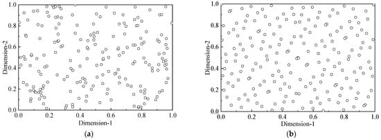
Figure 1.
Distribution of two-dimensional sampling results: (a) Monte Carlo sampling; (b) Sobol sequence sampling.
Therefore, in this study, Sobol sequence sampling is used to generate samples subject to uniform distribution in [0, 1] space and then transformed to a standard normal distribution vector through its inverse function using Equation (24).
where is the inverse function of standard normal distribution.
Through the function of Pearson correlation coefficients, R, samples subjected to the multivariate standard normal distribution function can be obtained. According to Equation (16), they can be converted into random numbers that obey a uniform distribution on [0, 1], without a change in R. The samples obeying the edge distribution of the original random variables are then obtained using the inverse function of the cumulative distribution. The detailed steps are shown in Figure 2.

Figure 2.
CSSC sampling process.
2.3. Multi-Lane Traffic Load Clustering Model
Vehicle parameters, such as vehicle weight, axle weight, and axle base, and their parameter distribution conform to certain statistical regularities [27]. Based on the established clustering and sampling method, random traffic flow can be simulated according to the macro distribution characteristics obtained by the traffic monitoring system. The sampling process for traffic flow is shown in Figure 3. The traffic parameters were clustered using the improved k-means method to achieve traffic volume, traffic speed, and vehicle type proportion. Then, the axle distance and axle weight of each vehicle are generated by the CSSC method, where the proportion of the hourly traffic volume and vehicle type in each lane obtains the number of each vehicle type. Finally, each vehicle is combined with randomly generated parameter samples based on the statistical characteristics, and the sequence of vehicle samples is randomly sorted. Accurate analysis and evaluation of the traffic flow load effect can be achieved based on the proportion of each cluster in the operation period.
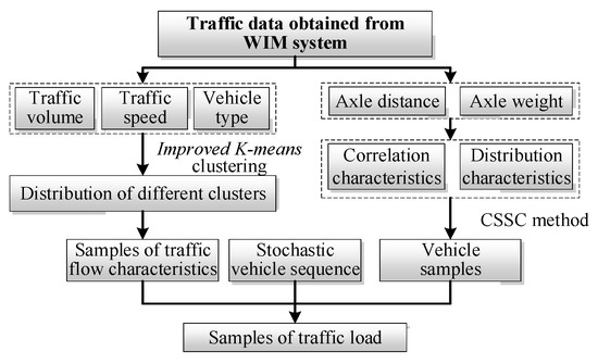
Figure 3.
Simulation process of stochastic traffic flow.
3. Prototype Bridge and Traffic Load
3.1. Bridge Information
A long-span suspension bridge was selected as the research subject to analyze the dynamic response under simulated traffic flow. The bridge was a single-span steel-concrete composite girder suspension bridge. The section layout is shown in Figure 4. The span of the main cable was arranged as (250 + 838 + 215) m, and the sagittal span ratio of the midspan main cable was 1/10. The central transverse spacing of the two main cables in midspan is 26.0 m. Two flexible central buckles are set near both sides of the middle span of each main cable to form a cable–beam connection. The stiffening girder adopted a steel-concrete composite structure wherein the steel beam was attached to the concrete deck using shear nails, as shown in Figure 5. The full width of the stiffening girder is 33.2 m, the center height is 2.8 m, and the center spacing of the longitudinal beam webs on both sides is 26.0 m. The reinforced concrete bridge deck was 25.0 m wide and 0.22 m thick.

Figure 4.
Layout of the prototype bridge.

Figure 5.
Section of stiffening girder section.
A three-girder bridge model was established using ANSYS 18.0 software to simulate the structural characteristics. The BEAM4 element was used to simulate the main stringer, small stringer, and the pylon. The LINK10 element was used to simulate the cable components. The girder, pylon, and cable components have 1836 BEAM4 elements, 82 BEAM4 elements, and 279 LINK10 elements, respectively. Only the mass of bridge deck pavement was considered as it contributed minimally to the stiffness of the stiffening girder. The stress stiffening of the suspenders was conducted in accordance with the measured force.
3.2. Traffic Monitoring Data
Traffic flow on bridges is a complicated and changeable load with different traffic densities, volumes, and speeds. These parameters directly influence the response of bridges. In this study, traffic flow data collected using the WIM system was used to analyze the bridge’s dynamic response under vehicle load. The monitoring data included vehicle data for 31 days. Vehicles were divided into five types according to the number of axles, that is, T-1 to T-6. Figure 6 and Figure 7 show the hourly traffic volume and its distribution in each lane, respectively. Lane 3 is the passing lane occupied by two-axle vehicles, whereas multi-axle vehicles mostly drive in lane 1; the hourly traffic volume in each lane exhibits considerable differences for different traffic speeds. Researchers typically consider traffic density as an indicator to simulate based on long-term overall statistical results [28,29]. Figure 8 displays the distribution of traffic volume, traffic speed, and proportion of V6 in lane 1, all of which obey a multimodal distribution and have different distribution characteristics. Based on long-term statistical features, the load effect of the traffic flow may be simulated in a limited manner because the complex time-varying characteristics of each parameter are concisely considered.
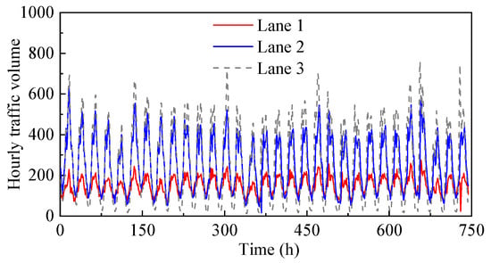
Figure 6.
Hourly traffic volume of WIM data.
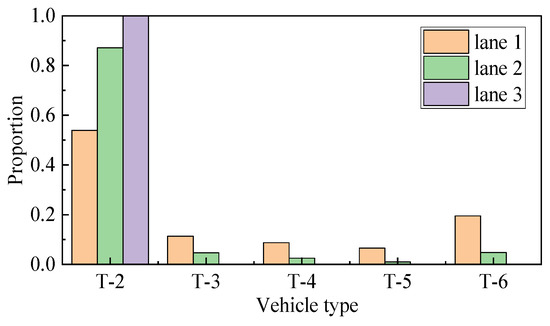
Figure 7.
Proportion of each vehicle type.

Figure 8.
Distribution of traffic parameters of WIM data: (a) traffic volume; (b) traffic speed; (c) proportion of T-6.
Figure 9 shows the scatter distribution of axle weight and distance for six-axle vehicles. It is observed that the axle weight and axle distance of the two rear axles have a noticeable correlation, whereas the correlation between the front axle and the rear axle is weak.
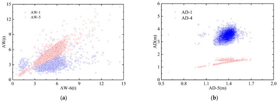
Figure 9.
Distribution of vehicle axle weight and axle distance: (a) axle weight; (b) axle distance.
4. Results and Discussion
4.1. Simulated Traffic Flow
Based on the clustering algorithm, six parameters in the traffic flow data of the three lanes, including traffic volume Q and traffic flow speed V, were selected as cluster analysis parameters. Table 1 lists the correlation coefficient for each parameter, the closer it is to 1, the stronger the correlation is. The weight of each dimension is calculated using Equation (6). The quality of the clustering results was measured using the Davies-Bouldin index [30], which tended to be stable when k reached 5. Figure 10 shows the distribution of the clustering results. Figure 11 displays the distribution of the traffic volume, traffic speed, and vehicle proportion in cluster 1. Although the proportion of vehicle types is not clustered, the distribution of vehicle types affects traffic volume and speed. The distribution of traffic parameters in the cluster showed a unimodal distribution after clustering, indicating the same distribution characteristics.

Table 1.
Pearson correlation coefficient of each parameter.
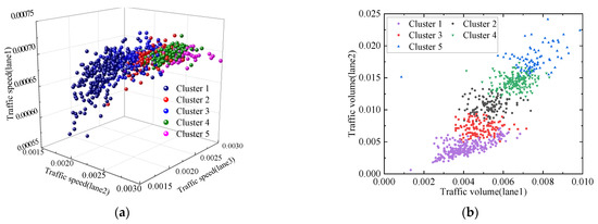
Figure 10.
Cluster processing results: (a) three-dimensional distribution of traffic speed; (b) two-dimensional distribution of traffic volume.

Figure 11.
Distribution of traffic parameters of cluster 1: (a) traffic volume; (b) traffic speed; (c) proportion of T-6.
Following the clustering analysis, distribution fitting was performed for the characteristics of the vehicle flow parameters in each cluster (Table 2). Table 2 lists the characteristic parameters of each cluster, which obey the normal, log-normal, and Weibull distributions. Significant differences were observed in the values of the parameters of each cluster, proving the effectiveness of clustering analysis in dealing with the distribution characteristics of traffic flow. The traffic volume of Cluster 5 was the largest, and that of Cluster 2 was the smallest. The parameter distributions of the clusters differ from each other, especially in terms of traffic volume. It is determined by the composition of vehicle types, wherein the proportion of multi-axle vehicles play a decisive role. In Lane 3, which is the passing lane, the share of two-axle vehicles accounts for more than 99%, and the difference in the proportion of vehicle types is neglected. According to the distribution parameters of each cluster, the multi-lane traffic flow can be simulated and used to analyze the bridge’s response.

Table 2.
Distribution parameters of each cluster.
A clustering algorithm is used to separate the traffic composition into different clusters based on the state parameters to consider the characteristics of the traffic flow. The samples in each cluster have consistent parameter characteristics. Based on the distribution characteristics of traffic flow obtained by cluster analysis, the total number of vehicles, speed of traffic flow, and proportion of vehicle types in each cluster are sampled by the Monte Carlo method, and the distance between vehicles can be obtained by classical traffic flow theory, as shown in Equation (25).
where Q denotes the traffic volume, K denotes the traffic density, and V denotes the traffic speed.
Q = K·V
Figure 12 shows 3000 axle weight and distance samples of six-axle vehicles generated by the CSSC method, which is similar to Figure 9. This demonstrates that the CSSC sampling method can adequately represent the correlation of the original samples.
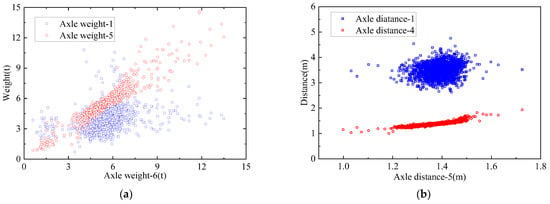
Figure 12.
Samples by CSSC method: (a) samples of axle weight; (b) samples of axle distance.
4.2. Response under Traffic Load
To analyze the vehicle–bridge interaction, the traffic loads of different clusters were generated based on the proposed method. The process is as follows: (1) collect traffic load characteristics using the WIM system and then cluster them; (2) fit the characteristics of traffic flow parameters based on cluster analysis and generate random traffic flow samples using CSSC sampling; and (3) feed traffic flow into the traffic flow bridge coupling analysis system to determine the dynamic response of the bridge. Based on the proposed traffic simulation method, the traffic volumes of different clusters were generated according to their hourly characteristics, and the axle load and wheelbase of vehicles were simulated accordingly. The generated traffic volumes for each cluster were 211, 705, 535, 1071, and 1240. The opposite lane generates a traffic flow to achieve two-way loading. The bridge response under each cluster of traffic flow can be determined by the established vehicle–bridge coupling analysis system, wherein the principle and vehicle parameter dynamic model parameters can be observed in the published literature [31]. Road surface roughness is described by a power spectral density function, that can be generated through Fourier inversion [32].
Figure 13 and Figure 14 show the response of the girder bending moment and vertical displacement at the midspan. To demonstrate the response difference under different cluster traffic flows more intuitively, responses under Clusters 1, 2, and 5 were selected from low to high traffic volumes. The differences in the responses under different clusters can be observed; the girder bending moment under Cluster 2 is the greatest and reaches 28,937.6 . The maximum vertical displacement of the main beam reached 0.404 m, in Cluster 3. Figure 15 shows the longitudinal displacement response of the girder end. As the amplitude of the longitudinal reciprocating motion of the main beam is small, the difference in the time-history curve is not apparent, and the cumulative displacement is shown in Figure 15b. The growth rate of the cumulative displacement in Cluster 5 was significantly higher than that of the other clusters. This difference may directly influence the fatigue life of bridge components, such as expansion joints.

Figure 13.
Girder bending moment under different clusters: (a) time history response; (b) extreme value.

Figure 14.
Vertical girder displacement under different clusters: (a) time history response; (b) extreme value.

Figure 15.
Longitudinal girder displacement under different clusters: (a) time history response; (b) cumulative displacement.
Figure 16 and Figure 17 show the time history response of axial and bending stress variation of a short suspender at midspan. As the bending stress cannot be extracted by the Link 10 element, it was calculated according to the Wyatt formula and experimental results [33,34]. The stress has differences such that peak values appear in different clusters. The maximum bending stress reached 50.676 MPa in Cluster 5, whereas the minimum value of 28.206 MPa appears in Cluster 4. The maximum axial stress reached 67.115 MPa in Cluster 1, which has the smallest traffic volume. It is primarily due to the large dead weight of long-span suspension bridges and the small spacing of suspenders. The axial force on a suspender is primarily affected by the weight of a single vehicle. The bending stress is affected by the traffic load effect.
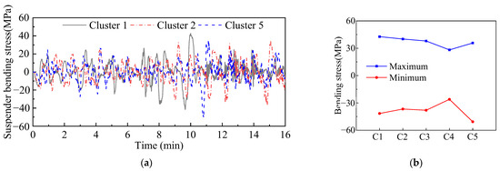
Figure 16.
Suspender bending stress under different clusters: (a) time history response; (b) extreme value.

Figure 17.
Suspender axial stress under different clusters: (a) time history response; (b) extreme value.
These results show an extreme response under different traffic flows. To explain the difference in long-term effects under different traffic flows, the variable-amplitude stress was transformed into an equivalent stress. Figure 18 shows the suspender stress under Cluster 1, processed using the rain-flow counting method. When the stress ranges and number of cycles is obtained, the equivalent stress range can be calculated based on the Paris criterion, as in Equation (26).
where and are the stress range and the corresponding number of cycles, m is the coefficient of Paris law, and has the value 3.
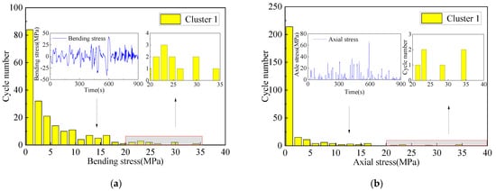
Figure 18.
Stress distribution of rain flow counting: (a) time history response; (b) extreme value.
The equivalent stresses of suspender bending and axial stresses are listed in Table 3. The maximum equivalent bending stress and axial stress were 16.068 MPa and 10.542 MPa, whereas the minimum values were 9.429 MPa and 8.679 MPa, respectively. The maximum equivalent stress appears in Cluster 3, and is not consistent with the peak values. Because the stress response is closely related to the fatigue life of suspenders, the response under different traffic flows must be considered in the fatigue analysis of suspenders because of the noticeable difference. The established traffic flow simulation method can consider traffic flow effects at different intensities, which is beneficial for achieving an accurate evaluation in the long-term evaluation of bridge component performance.

Table 3.
Equivalent stress and maximum value of suspender (MPa).
5. Conclusions
In this study, a random traffic load simulation method for long-span bridges is established based on monitoring traffic data. To analyze the load level composition during service, an improved k-means clustering algorithm was established to process traffic characteristics. Consequently, a CSSC sampling method that considers parameter correlation was established based on Sobol sequence sampling. Finally, the generated stochastic traffic flow was used to analyze the dynamic response of a long-span suspension bridge under the traffic flow of different clusters. The following conclusions were drawn:
1. An improved k-means clustering algorithm was constructed by introducing the CRITIC weight and sample weight to reduce the correlation between sample dimensions and the interference of discrete points. Based on the clustering algorithm, the traffic flow can be separated into clusters with different traffic volumes and speeds. The key parameters of traffic flow and the proportion of vehicle types in each cluster subject to specific distribution characteristics, which are optimized from the multi-peak distribution to the single-peak distribution.
2. The CSSC sampling method was established based on the Sobol sequence and Copula joint function theory. Based on the correlation coefficient matrix of the original sample, the simulation of the vehicle axle load and axle distance considering parameter correlation can be achieved by CSSC. Combined with the clustering results, a refined stochastic traffic flow simulation method is established and used to reconstruct the traffic load. The loading traffic flow can effectively avoid the simple division of traffic intensity and consider the daily traffic characteristics.
3. There are evident differences in the bridge responses under different clusters of traffic flow. Typical indicators, such as the girder bending moment, girder displacement, and suspender stress, show noticeable differences in extreme values under different clusters. The equivalent stresses exhibit clear differences, and the maximum equivalent stress appears in different clusters from that of the peak values. These differences directly influenced the long-term evaluation of these components. The traffic flow density must be considered to achieve an accurate evaluation in the long-term evaluation of bridge component performance.
The multi-lane traffic load model has the capability to model long-term traffic variation trends and characteristic parameters. However, if the bridge is extremely long, aerodynamic forces should be considered. The interaction between traffic loading and aerodynamic loading could further compromise the safety of a bridge; further research and relevant investigations are required in the analysis and evaluation of bridge responses under external loads.
Author Contributions
Conceptualization, Y.Z. (Yue Zhao) and Y.Z. (Yiyun Zhu); methodology, Y.Z. (Yiyun Zhu); software, X.G.; validation, X.G. and B.S.; formal analysis, X.G.; investigation, Y.S.; resources, Y.Z. (Yue Zhao); data curation, X.G.; writing—original draft preparation, Y.Z. (Yue Zhao); writing—review and editing, X.G.; visualization, B.S.; supervision, Y.Z. (Yiyun Zhu); project administration, Y.Z. (Yue Zhao); funding acquisition, Y.Z. (Yue Zhao). All authors have read and agreed to the published version of the manuscript.
Funding
This research was funded by the Natural Science Basic Research Program of Shaanxi (Program No. 2022JQ-336); the open fund of Shaanxi Provincial Key Laboratory (Chang’an University) of Highway Bridges and Tunnels (Program No. 300102212509); the Foundation of Xi’an University of Technology (Grant no. 256082109).
Data Availability Statement
Some or all data, models, or codes that support the findings of this study are available from the corresponding author upon reasonable request.
Conflicts of Interest
The authors declare no conflict of interest.
References
- Zhou, R.; Ge, Y.J.; Yang, Y.X.; Du, Y.L.; Zhang, L.H. Wind-induced nonlinear behaviors of twin-box girder bridges with various aerodynamic shapes. Nonlinear Dyn. 2018, 94, 1095–1115. [Google Scholar] [CrossRef]
- Guo, T.; Liu, J.; Zhang, Y.; Pan, S. Displacement monitoring and analysis of expansion joints of long-span steel bridges with viscous dampers. J. Bridge Eng. 2015, 20, 4014099. [Google Scholar] [CrossRef]
- Liu, Z.X.; Guo, T.; Huang, L.Y.; Pan, Z.H. Fatigue life evaluation on short suspenders of long-span suspension bridge with central clamps. ASCE’s J. Bridge Eng. 2017, 22, 04017074. [Google Scholar] [CrossRef]
- Yuan, A.M.; Yang, T.; Xia, Y.F.; Qian, L.F. Replacement Technology of Long Suspenders of Runyang Suspension Bridge. China J. Highw. Transp. 2021, 34, 289–297. [Google Scholar]
- Kafle, B.; Zhang, L.; Mendis, P.; Herath, N.; Maizuar, M.; Duffield, C.; Thompson, R. Monitoring the dynamic behavior of the merlynston creek bridge using interferometric radar sensors and finite element modeling. Int. J. Appl. Mech. 2017, 9, 1750003. [Google Scholar] [CrossRef]
- César, C.M.; Juan, R.C. A Comprehensive Traffic Load Model for Bridge Safety Checking. Struct. Saf. 1997, 19, 339–359. [Google Scholar]
- Chen, Y.B.; Feng, M.Q.; Tan, C.A. Modeling of Traffic Excitation for System Identification of Bridge Structures. Comput.-Aided Civ. Infrastruct. Eng. 2010, 21, 57–66. [Google Scholar] [CrossRef]
- Chen, S.R.; Wu, J. Modeling Stochastic Live Load for Long-span Bridge Based on Microscopic Traffic Flow Simulation. Comput. Struct. 2011, 89, 813–824. [Google Scholar] [CrossRef]
- Jabari, S.E.; Liu, H.X. A Stochastic Model of Traffic Flow: Theoretical Foundations. Transp. Res. Part B 2012, 46, 156–174. [Google Scholar] [CrossRef]
- Han, W.; Liu, X.; Gao, G.; Xie, Q.; Yuan, Y. Site-specific extra-heavy truck load characteristics and bridge safety assessment. J. Aerosp. Eng. 2018, 31, 04018098. [Google Scholar] [CrossRef]
- Wang, C.S.; Chen, H.Z.; Chen, A.R.; Lei, X. 3D finite-element model simulation and remaining fatigue life assessment of existing steel bridges. J. Chang‘an Univ. (Nat. Sci. Ed.) 2004, 24, 43–47. [Google Scholar]
- Zong, Z.H.; Li, F.F.; Xia, Y.F.; Yuan, W.W. Study of vehicle load models for Xinyi River Bridge Based on WIM data. Bridge Constr. 2013, 43, 29–36. [Google Scholar]
- Han, W.S.; Chen, A.R. Three-dimensional coupling vibration of wind-vehicle-bridge systems under random traffic flow. China Civ. Eng. J. 2008, 9, 97–102+2. [Google Scholar]
- Bernard, E.; O’Brien, E. Monte carlo simulation of extreme traffic loading on short and medium span bridges. Struct. Infrastruct. Eng. 2013, 9, 1267–1282. [Google Scholar]
- Cheng, J.; Xie, Y.; Zhang, J. Industry structure optimization via the complex network of industry space: A case study of Jiangxi Province in China. J. Clean. Prod. 2022, 338, 1306024. [Google Scholar] [CrossRef]
- Cheng, J. Analysis of the factors influencing industrial land leasing in Beijing of China based on the district-level data. Land Use Policy 2022, 122, 106389. [Google Scholar] [CrossRef]
- Cheng, J.; Luo, X.W. Analyzing the land leasing behavior of the government of Beijing, China, via the multinomial logit model. Land 2022, 11, 376. [Google Scholar] [CrossRef]
- Lantz, B. Machine Learning with R; Packt Publishing: Birmingham, UK, 2013. [Google Scholar]
- Yang, Z.T.; Huang, X.F.; Fang, G.H.; Ye, J.; Lu, C.X. Benefit evaluation of East Route Project of South to North Water Transfer based on trapezoid cloud model. Agric. Water Manag. 2021, 254, 106960. [Google Scholar] [CrossRef]
- Chiu, S.; Cheng, J.J. Automatic Generation of Fuzzy Rulebase for Robot Arm Posture Selection. In Proceedings of the First International Joint Conference of The North American Fuzzy Information Processing Society Biannual Conference, San Antonio, TX, USA, 18–21 December 1994; pp. 436–440. [Google Scholar]
- Cheng, J.; Yin, P. Analysis of the complex network of the urban function under the lockdown of COVID-19: Evidence from Shenzhen in China. Mathematics 2022, 10, 2412. [Google Scholar] [CrossRef]
- Tan, G.; Kong, Q.; Wang, L.; Wang, X.; Liu, H. Reliability evaluation of hinged slab bridge considering hinge joints damage and member failure credibility. Appl. Sci. 2020, 10, 4824. [Google Scholar] [CrossRef]
- Papaefthymiou, G.; Kurowicka, D. Using Copula for modeling stochastic dependence in power system uncertainly analysis. IEEE Trans Power Syst. 2009, 24, 40–49. [Google Scholar] [CrossRef]
- Li, M.; Liu, Y.; Yang, X.S. Random Vehicle Flow Load Effect Considering Axle Load. J. Zhejiang University. Eng. Sci. 2019, 53, 78–88. [Google Scholar]
- Dimov, I.; Georgieva, R.; Ostromsky, T.; Zlatev, Z. Advanced algorithms for multidimensional sensitivity studies of large-scale air pollution models based on sobol sequences. Comput. Math. Appl. 2013, 65, 338–351. [Google Scholar] [CrossRef]
- Joe, S.; Kuo, F.Y. Constructing Sobol’ sequences with better two-dimensional projections. SIAM J. Sci. Comput. 2008, 30, 2635–2654. [Google Scholar] [CrossRef]
- Han, W.S.; Li, Y.W.; Qiao, L. Moving Load Identification Based on Vehicle-bridge Coupling Vibration Theory. China J. Highw. Transp. 2013, 26, 74–86. [Google Scholar]
- Wang, F.Y.; Xu, Y.L. Traffic Load Simulation for Long-Span Suspension Bridges. J. Bridge Eng. 2019, 24, 05019005. [Google Scholar] [CrossRef]
- Liang, Y.Z.; Xiong, F. Multi-parameter Dynamic Traffic Flow Simulation and Vehicle Load Effect Analysis based on Probability and Random Theory. KSCE J. Civ. Eng. 2019, 23, 3581–3591. [Google Scholar] [CrossRef]
- Wang, C.; Gao, Y.H. Dynamic Reconfiguration of Distribution Network Based on Optimal Fuzzy C-means Clustering and Improved Chemical Reaction Optimization. Proc. CSEE 2014, 34, 1682–1691. [Google Scholar]
- Zhao, Y.; Huang, P.M.; Long, G.X.; Yuan, Y.G.; Sun, Y. Influence of Fluid Viscous Damper on the Dynamic Response of Suspension Bridge under Random Traffic Load. Adv. Civ. Eng. 2020, 2020, 1857378. [Google Scholar] [CrossRef]
- ISO-8608; KS Association. Mechanical Vibration-Road Surface Profiles-Reporting of Measured Data. International Organization for Standardization (ISO): Geneva, Switzerland, 1995.
- Wyatt, T.A. Secondary Stress in Parallel Wire Suspension Cables. J. Struct. Div. 1960, 86, 37–59. [Google Scholar] [CrossRef]
- Kondoh, M.; Okuda, M.; Kawaguchi, K.; Yamazaki, T. Design Method of A Hanger System for Long-Span Suspension Bridge. J. Bridge Eng. 2001, 6, 176–182. [Google Scholar] [CrossRef]
Disclaimer/Publisher’s Note: The statements, opinions and data contained in all publications are solely those of the individual author(s) and contributor(s) and not of MDPI and/or the editor(s). MDPI and/or the editor(s) disclaim responsibility for any injury to people or property resulting from any ideas, methods, instructions or products referred to in the content. |
© 2023 by the authors. Licensee MDPI, Basel, Switzerland. This article is an open access article distributed under the terms and conditions of the Creative Commons Attribution (CC BY) license (https://creativecommons.org/licenses/by/4.0/).