ML-k’sNN: Label Dependent k Values for Multi-Label k-Nearest Neighbor Rule

Abstract

Multi-label classification as a data mining task has recently attracted increasing interest from researchers. Many current data mining applications address problems with instances that belong to more than one category. These problems require the development of new, efficient methods. Multi-label k-nearest neighbors rule, ML-kNN, is among the best-performing methods for multi-label problems. Current methods use a unique k value for all labels, as in the single-label method. However, the distributions of the labels are frequently very different. In such scenarios, a unique k value for the labels might be suboptimal. In this paper, we propose a novel approach in which each label is predicted with a different value of k. Obtaining the best k for each label is stated as an optimization problem. Three different algorithms are proposed for this task, depending on which multi-label metric is the target of our optimization process. In a large set of 40 real-world multi-label problems, our approach improves the results of two different tested ML-kNN implementations.

1. Introduction

Many modern applications involve vast amounts of data that need to be classified into increasingly complex categorization schemes in which one data instance may simultaneously belong to several topics. This task is typically termed multi-label learning [1,2]. In contrast with single label classification, where each instance is associated with only one class, multi-label classification is concerned with learning from instances in which each instance can be associated with multiple labels. Many multi-label learning algorithms have been developed and applied to diverse problems: text categorization [3,4], the automatic annotation of multimedia contents [5], web mining [6], rule mining [7], cheminformatics [8], bioinformatics [9], information retrieval [10] and scientific applications [11] among others.

Examples of multi-label problems appear in almost any application field. For instance, in extracting the aspects of restaurant reviews from social network comments. In this context, the author of the text may mention none or all aspects of a preset list, such as, service, food, anecdotes, price, and ambiance. When classifying text by the topics included any text can contain one or several topics. In predicting subcellular localization of proteins [12] each protein can be localized in more than one part of the cell. In sentiment analysis a text can be classified as containing more than one sentiment at the same time [13].

The key challenge of multi-label learning is taking advantage of the correlations among labels to address the exponential growth of the label space as the number of distinct labels increases; when the number of distinct labels is q, the label space is $2^q$. One of the best-performing methods in multi-label learning is the adaptation of the k-nearest neighbors for multi-label datasets, the Multi-Label k-Nearest Neighbors (ML-kNN) [14] method. There are other adaptations of k-NN based on a binary relevant approach where the base classifier is a k-NN rule [15]. Any advance in the ML-kNN method is relevant as it is able to achieve very good performance, improving the results of much more complex algorithms [16].

ML-kNN uses the k nearest neighbors of every instance to predict the a posteriori probability of each label. However, the distribution of the labels across a particular dataset are very different for each label [17]. The algorithm is less accurate when the number of labels in the training set is not balanced and when the training instances are unevenly distributed in space [18]. In those cases, using the same value of k for all labels might be a suboptimal approach. The multi-label nature of ML-kNN does not depend on using the same k for all labels, so we propose the use of a different k for each label. We name this method “Multi-Label k’s-Nearest Neighbors” (ML-k’sNN).

In ML-k’sNN, instead of using a single k value for all labels, we use a vector $\mathbf{k}=(k_1,k_2,\dots ,k_q)$. A method for obtaining $\mathbf{k}$ must be devised to derive a useful approach. We state the problem as an optimization task and propose three different algorithms. The contribution of our paper is two-fold. Firstly, we have devised a new definition of ML-kNN adapted to the use of different values of k depending on each label. Secondly, we have developed a method for obtaining the optimal value of each k for every label. In a large set of 40 problems, we compare our method with two different implementations of standard ML-kNN and achieve a significant improvement. A further experiment is carried out to compare our proposal with ten different variants of ML-kNN. We have also carried out different studies on the behavior of our proposal depending on characteristics of the datasets such as number of features, number of labels and label diversity.

Furthermore, we have combined ML-k’sNN with instance selection and showed how our proposal is able to achieve better results than standard ML-kNN with a reduction ability above 95%. Finally, we have also shown the ability of our method to be adapted to other instance-based multi-label methods, such as LAML-kNN, with very good results.

The remainder of this paper is organized as follows: Section 2 describes the existing related work; Section 3 describes our proposal in depth; Section 4 explains the experimental setup; Section 5 presents and discusses the experimental results and, finally, Section 6 summarizes the conclusions of our work.

2. Related Work

Since ML-kNN was first developed [14], several modifications and improvements have been proposed. Xu [19] proposed and adaptive method based on quadratic programming to weight the votes of the different neighbors. Wang et al. [20] proposed a locally adaptive multi-label k-nearest neighbor (LAML-kNN) method where the instances are first clustered into different groups and then each cluster is separately processed to obtain the a posteriori probabilities. Jiang et al. [18] developed a weighted modification of ML-kNN where different weights are assigned to each label according to the proportion of labels and the mutual information regarding the spatial distribution of unseen instances to training instances. The author states that this method can reduce the probability of misjudging the unseen instance’s label set. This method can easily adapted to our proposal using a different value of k for each label together with the corresponding label weight. Wang et al. [21] proposed a multi-label classification algorithm based on k-nearest neighbors and random walk. This method constructs the set of vertices from a random walk graph for k-nearest neighbor training of samples of certain test data and the edge set of correlations among the labels of the training samples. Although this method can also be adapted to our philosophy its computational cost would be too high as the original method has serious scalability problems.

Other methods have been developed to improve ML-kNN. Younes et al. [22] proposed a dependent multi-label k-nearest neighbors (DMLk-NN) algorithm to take label association into account. While predicting the relevance of a label ${\lambda }_l$ for ${\mathbf{x}}_t$, along with the label ${\lambda }_l$, DML-kNN utilises all the other labels ${\lambda }_q\in \mathcal{L}-\left\{{\lambda }_l\right\}$ of the datapoints in the neighbor of the new datapoint ${\mathbf{x}}_t$. As for the previous two methods, DML-kNN can be adapted to use label dependent k values with almost no modifications. Pakrashi and Mac Namee [23] proposed Stacked-MLkNN, which follows the stacking methodology [24].

Using a fuzzy approach, Lin and Chen [25] developed Mr.KNN (Soft Relevance for Multi-label Classification) which combines a fuzzy c-means algorithm with a voting mechanism based on the k-nearest neighbors of every sample. The method voting stage can also be adapted to our label dependent approach. Vluymans et al. [26] developed a fuzzy rough multi-label classifier, FRONEC (fuzzy rough neighborhood consensus).

On a different task, the concept of label specificity has been also applied for feature selection for multi-label datasets. Hang and Zhang [27] developed a method called Collaborative Learning of label semantIcs and deep label-specific Features (CLIF) for multi-label classification.

As showed above, one of the advantages of our proposal is that, as it modifies the basic definition of the standard ML-kNN method, it can be applied to any other implementation of the method, such as those cited above. In the experiments, we will compare standard ML-kNN and LAML-kNN. Although it could applied to other Ml-kNN methods we restrict ourselves to two implementations to avoid too repetitive experiments.

3. Multi-Label $\mathit{k}$’s-Nearest Neighbors (ML-k’sNN)

Formally, we define a multi-label problem as follows [2]: Let T be a multi-label evaluation dataset consisting of p multi-label instances ${\mathbf{x}}_i$ and their associated label set $y_i$, where $T=\left\{({\mathbf{x}}_i,y_i)\right\},1\le i\le p$, $({\mathbf{x}}_i\in X,y_i\in \mathcal{Y}={\{0,1\}}^q)$ with a label set L, where $\left|L\right|=q$. Let h be a multi-label classifier and $h\left({\mathbf{x}}_i\right)={\{0,1\}}^q$ be the set of labels predicted by h for the instance ${\mathbf{x}}_i$. Let $f({\mathbf{x}}_i,y_i)$, ${\mathbf{x}}_i\in X$, $y_i\in \mathcal{Y}$ be a real-valued function $f:X\times \mathcal{Y}\to R$. A successful learning system would tend to output larger values from function f for the labels in $y_i$ versus those not in $y_i$. The real-valued function f can be easily transformed to a ranking function, $ran{k}_f({\mathbf{x}}_i,y_i)$, where $ran{k}_f$ is the predicted rank of label $y_i$ for instance ${\mathbf{x}}_i$. For example, if f represents the probability of every instance of being relevant, which is the case for many multi-label classifiers, $ran{k}_f({\mathbf{x}}_i,y_i)$ can be obtained assigning to $y_i$ its position within the sorted values of f. $h\left({\mathbf{x}}_i\right)$ can be obtained from $f\left({\mathbf{x}}_i\right)$ when an appropriate threshold is set.

As an example if we have a problem with $q=5$, and instance $\mathbf{x},\mathbf{y}$ is composed for a sample $\mathbf{x}$ of a certain dimension d, $\mathbf{x}\in {\mathcal{R}}^d$ and $\mathbf{y}={\{0,1\}}^5$. $\mathbf{y}=\left(01100\right)$ means that labels 2 and 3 are relevant for instance $\mathbf{x}$ and labels 1, 4 and 5 are not relevant.

Our method is based on two different ideas. First, we modify ML-kNN to use a different $k_l$ value for the prediction of l-th label. We must mention that the use of multiple values for the number of neighbors k, one per label, does not modify the computational cost of the method at testing stage as both methods, ML-kNN and ML-k’sNN, must obtain the distance of the query instance to all the prototypes. The second idea describes a way to obtain the $k_l$ values for each label $l\in \mathcal{Y}$. The first idea is rather straightforward, the modification affects only the number of neighbors considered when obtaining the different probabilities for each label. Algorithm 1 depicts the proposed approach. Thus, once the vector of $\mathbf{k}$ values is obtained, the algorithm is similar to ML-kNN. We termed our method Multi-Label k’s-Nearest Neighbors (ML-k’sNN) as it uses a variety of k values instead of just one. In this way, we will never have a ML-4’sNN in the same sense that a ML-4NN, as the number of different k’s will depend on the number of labels.

As in the standard ML-kNN algorithm, $P\left(H_1^l\right)$ $\left(P\right(H_O^l\left)\right)$ is the prior probability of label l being relevant (irrelevant) and $P\left(E_j^l\right|H_1^j)$ ($P\left(E_j^l\right|H_0^j)$) is the posterior probability of label l being relevant (irrelevant), $N_j\left({\mathbf{x}}_i\right)$ is the set of neighbors of ${\mathbf{x}}_i$ for label j.

Algorithm 1: ML-k’sNN: Multi-label k’s nearest neighbors algorithm.

Once we have defined the new algorithm, we must establish how $\mathbf{k}$ is obtained. In the standard ML-kNN, k is either arbitrarily fixed or obtained using cross-validation. It is evident that letting the expert to fix an a priori value of $k=(k_1,k_2,\dots ,k_q)$ for every label is unreasonable as there is not way of knowing optimal values for every label. Thus, we must design a method that establishes the best values for $k_i,i\in \{1,\dots ,q\}$. We define this task as an optimization problem.

This optimization problem is defined in the following way: first, we set an interval from which the values of $\mathbf{k}$ will be chosen $[k_{\min },k_{\max }]$. Then, a certain metric, m (for multi-label performance metrics refer to Zhang and Zhou [2]), is chosen to evaluate each vector of $k^{\prime }$s. Our algorithm must optimize m over all the possible values of $\mathbf{k}$. As a base algorithm, we first define a single-label approach to the problem. In this algorithm, we obtain $k_i$ as the optimum value for a standard single-label k-NN algorithm used to classify only label $Y_i$. This single-label approach is named ML-k’sNN.SL (shown in Algorithm 2). However, we must bear in mind that this algorithm does not optimize the value of metric m, as it is based on a single-label approach.   

Algorithm 2: ML-k’sNN.SL: Multi-label k’s nearest neighbors algorithm single-label approach.

Thus, we must devise a multi-label approach. However, when the optimization problem is addressed as a multi-label problem, the method for obtaining the vector of $k^{\prime }$s depends on the metric. For multi-label classification metrics, the prediction of whether a certain label $Y_l$ is relevant to a given instance depends only on the value of $k_l$. Thus, we can optimize the value of every $k_l$ independently and that guarantees the optimal value. However, for label ranking, the position of a label $y_l$ for an instance ${\mathbf{x}}_t$ depends on all the values of ${\mathbf{r}}_t$. In that case, we cannot obtain optimal values of $\mathbf{k}$ by independently searching over each label.

When we plan as optimization target a classification metric we must bear in mind is that for every instance ${\mathbf{x}}_t$, we will use the classification given by ${\mathbf{y}}_t$ as defined in Algorithm 1. The result of the testing stage of the algorithm is the prediction of relevant and irrelevant labels for a test label ${\mathbf{x}}_t$, ${\mathbf{y}}_t$, and the ranking function for the query instance, ${\mathbf{h}}_t$, as defined above. This algorithm shows that ${\mathbf{y}}_t\left(l\right)$ depends only on $k_l$ to predict whether label l is relevant, while ${\mathbf{y}}_t\left(l\right)=arg{max}_{b\in \{0,1\}}P\left(H_b^l\right)P\left(E_{{\mathbf{C}}_t\left(l\right)}^l\right|H_b^l)$ does not depend on $k_l$. This observation means that any classification metric used for multi-label problems can be optimized by obtaining the optimal value for every $k_l$ independently. Thus, a simple way to optimize the given metric is to carry out a search for every $k_l$ separately. This method is fast and has the additional advantage of easy parallelization. The method is outlined in Algorithm 3. This method is named ML-k’sNN.ML, where ML stands for multi-label. This additional calculation of the optimal k for every label has a computational cost comparable with obtaining the optimal k for standard ML-kNN using cross-validation.   

Algorithm 3: ML-k’sNN.ML: Multi-label k’s nearest neighbors algorithm multi-label approach.

In several cases the performance of different values for k achieves the same value for the metric used. In such cases, we select, from among the equally best k’s, the nearest one to the best value for ML-kNN, obtained by 10-fold cross-validation.

However, if our optimization target is, or contains, a ranking metric, this procedure cannot be used. Although the prediction of every label is independent from the prediction of the rest of the labels in ML-kNN, the ranking of the labels does depend on all the obtained values. In such a case, an independent search for each $k_l$ cannot be performed. We must search for the optimal vector of k values $\mathbf{k}$. In this case, we must optimize metric m for all possible vectors of k’s, $\mathbf{k}$, with $k_i\in \{k_{\min },k_{\max }\}$. Due to the size of the search space, an exhaustive search such as the one used in ML-k’sNN.ML is not feasible.

In such complex optimization processes, evolutionary computation has proven to be a very efficient tool. We propose a simple evolutionary algorithm where each solution is codified as a vector of integer values. The fitness of every individual is obtained using the method shown in Algorithm 1. New individuals were generated using BLX-$\alpha$ [28] crossover and no mutation was applied. We intentionally use a very simple evolutionary method to avoid obscuring the results of our approach with the use of a very complex optimization process. This method is named ML-k’sNN.EC, where EC stands for evolutionary computation.

4. Experimental Setup

To produce a fair comparison between the standard ML-kNN algorithm and our proposal, we considered 40 datasets whose characteristics are shown in

Table 1. Description of the datasets.

	Dataset	Instances	Features	Labels	Cardinality	Density	Diversity	Proportion of Distinct Labels	MeanIR	CVIR	Source
1	bibtex	7395	1836	159	2.40	0.0151	1654	0.2237	12.50	0.4051	[29]
2	birds	645	271	19	1.86	0.0981	132	0.3761	5.41	0.8169	[29]
3	CAL500	502	68	174	26.04	0.1497	495	0.9861	20.58	1.0871	[29]
4	corel16k005	13,847	500	160	2.86	0.0179	1784	0.1288	34.94	0.7282	[29]
5	Corel5k	5000	499	373	3.52	0.0094	1453	0.2906	189.57	1.5266	[29]
6	enron	1702	1001	53	3.38	0.0637	753	0.4424	73.95	1.9596	[29]
7	EukaryoteGO	7766	12,689	22	1.15	0.0521	112	0.0144	45.01	1.4070	[30]
8	EukaryotePseAAC	7766	440	22	1.15	0.0521	112	0.0144	45.01	1.4070	[30]
9	genbase	662	1185	27	1.25	0.0464	32	0.0483	37.31	1.4494	[29]
10	HumanGO	3106	9844	14	1.19	0.0847	85	0.0274	15.29	1.0850	[30]
11	HumanPseAAC	3106	440	14	1.19	0.0847	85	0.0274	15.29	1.0850	[30]
12	LLOG-F	1460	1003	75	1.38	0.0183	278	0.2219	39.27	1.3106	[31]
13	medical	978	1449	45	1.25	0.0277	94	0.0961	89.50	1.1476	[31]
14	OHSUMED-F	13,929	1002	23	1.66	0.0723	1147	0.0823	7.87	0.8920	[31]
15	rcv1subset1	6000	47,236	101	2.88	0.0285	837	0.1395	54.49	2.0806	[29]
16	rcv1subset2	6000	47,236	101	2.63	0.0261	800	0.1333	45.51	1.7148	[29]
17	rcv1subset3	6000	47,236	101	2.61	0.0259	783	0.1305	68.33	2.9901	[29]
18	rcv1subset4	6000	47,236	101	2.48	0.0246	698	0.1163	89.37	2.3336	[29]
19	rcv1subset5	6000	47,236	101	2.64	0.0262	782	0.1303	69.68	2.6979	[29]
20	REUTERS-K500-EX2	6000	500	103	1.46	0.0142	618	0.1030	51.98	1.9707	[31]
21	SLASHDOT-F	3782	1079	22	1.18	0.0537	156	0.0412	17.69	2.4155	[31]
22	Stackex_chemistry	6861	540	175	2.11	0.0121	1452	0.2088	56.88	0.8964	[32]
23	Stackex_chess	1675	585	227	2.42	0.0106	508	0.3038	85.79	0.8167	[32]
24	Stackex_coffee	225	1763	123	1.99	0.0162	149	0.6622	27.24	0.5715	[32]
25	Stackex_cooking	10,491	577	400	2.25	0.0056	1712	0.1653	37.86	0.6513	[32]
26	Stackex_cs	9270	635	274	2.57	0.0094	1489	0.1613	85.00	0.7596	[32]
27	Stackex_philosophy	3971	842	233	2.28	0.0098	1072	0.2708	68.75	0.7989	[32]
28	Water-quality	1060	16	14	5.10	0.3644	824	0.7818	1.77	0.3016	[33]
29	Yahoo_Arts	7484	23,146	26	1.65	0.0636	599	0.0800	94.74	3.8059	[29]
30	Yahoo_Business	11,214	21,924	30	1.60	0.0533	233	0.0208	880.18	2.8112	[29]
31	Yahoo_Computers	12,444	34,096	33	1.51	0.0457	428	0.0344	176.70	1.9062	[29]
32	Yahoo_Education	12,030	27,534	33	1.46	0.0443	511	0.0425	168.11	1.7756	[29]
33	Yahoo_Entertainment	12,730	32,001	21	1.41	0.0673	337	0.0265	64.42	1.5398	[29]
34	Yahoo_Health	9205	30,605	32	1.64	0.0514	335	0.0364	653.53	1.9399	[29]
35	Yahoo_Recreation	12,828	30,324	22	1.43	0.0650	530	0.0413	12.20	1.3899	[29]
36	Yahoo_Reference	8027	39,679	33	1.17	0.0356	275	0.0343	461.86	2.0073	[29]
37	Yahoo_Science	6428	37,187	40	1.45	0.0362	457	0.0711	52.63	1.6349	[29]
38	Yahoo_Social	12,111	52,350	39	1.28	0.0328	361	0.0298	257.70	2.3431	[29]
39	Yahoo_Society	14,512	31,802	27	1.67	0.0619	1054	0.0726	302.07	4.5633	[29]
40	yeast	2417	103	14	4.24	0.3026	198	0.0819	7.20	1.8838	[29]

. These datasets represent a varied number of problems with different numbers of instances, features and labels. Furthermore, the label densities among the datasets are very different. The selection of the datasets was carried out with the aim of using a wide variety of problems in terms of instances, features, number of labels, label density and label cardinality. Datasets from different application fields were selected as well, such as text categorization, image classification and Bioinformatics.

The tables shows a detailed description of the characteristics of the datasets. The tables shows the number of instances of the datasets, the number of inputs, the number of labels, the label cardinality, the label density, the label diversity, the proportion of distinct labels, and MeanIR and CVIR measures [2,17]. The table also show the source of every dataset.

Regarding comparisons, we used the Wilcoxon test [34] as the main statistical test for comparing pairs of algorithms. For groups of methods, we first carry out an Iman–Davenport test to ascertain whether there are significant differences among methods. When the Iman–Davenport test rejects the null hypothesis, we can proceed with a post hoc Nemenyi test [35], which compares groups of methods.

Although there are several versions of ML-kNN [15,18,20], our proposal can be used to modify most of them. In our experiments, we used the original ML-kNN, and LAML-kNN. The source code, which was written in C and licensed under the GNU General Public License, and the datasets are freely available upon request from the authors.

For evaluating the classification performance of the different methods we used 10-fold cross-validation which is one of the most common methods in Machine Learning. k-fold cross-validation involves randomly dividing the set of observations into k groups, or folds, of approximately equal size. The first fold is treated as a validation set, and the method is fit on the remaining $k-1$ folds [36]. This process is repeated for each one of the k folds and the performance metrics reported are the average values over the k repetitions.

The evaluation of multi-label classification methods is more difficult because the prediction result for an instance is a set of labels, and the result can be fully correct, partially correct (with different levels of correctness) or fully incorrect [37,38,39]. The metrics can be divided into two major groups: example-based (EB) metrics and label-based (LB) metrics. The former group evaluates the learning system for each instance (example) separately and then obtains a unique measure for the average value across the test set.

There are many metrics defined in the literature [2]. Among them, we have chosen accuracy and F1 metrics to compare the results of the studied methods. The precision and recall metrics are not usually reported individually because each can always be maximized by selecting no relevant label or all labels as relevant. These two metrics are devoted to classification. We also consider three metrics used for measuring the ability of a classifier from the point of view of ranking the labels: coverage, ranking loss and average precision [2]. Finally, for label-based metric we report F1 micro averaged and F1 and macro averaged.

In the experiments, we show the results of using all of these metrics as well as the results of using a subset of them in certain cases. The use of different metrics is justified because they represent the performance of the models from different points of view.

5. Experimental Results

The first set of experiments was devoted to the comparison of ML-k’sNN and LAML-k’sNN against ML-kNN and LAML-kNN. As we stated in a previous section, we carry out a different procedure depending on whether the target metric is a classification metric or a ranking metric. The first set of experiments was carried out using classification metrics. As described above, we used accuracy, F1, the macro-averaged F1 and micro-averaged F1.

Table 2. Comparison of the different methods using accuracy metric.

		ML-kNN	ML-k’sNN.SL	ML-k’sNN.ML	LAML-kNN	LAML-k’sNN.ML
Mean		0.3440	0.3544	0.3606	0.3314	0.3617
Ranks		3.7500	2.8375	2.0500	4.1000	2.2625
	w/l		26/14	35/3	12/18	31/9
ML-kNN	p		0.0155	0.0000	0.1231	0.0000
	$R^{+}/R^{-}$		590.0/230.0	772.5/47.5	295.5/524.5	720.0/100.0
	w/l			25/14	10/30	24/16
ML-k’sNN.SL	p			0.1053	0.0006	0.1039
	$R^{+}/R^{-}$			530.5/289.5	153.0/667.0	531.0/289.0
	w/l				6/34	17/22
ML-k’sNN.ML	p				0.0000	0.4476
	$R^{+}/R^{-}$				103.0/717.0	353.5/466.5
	w/l					37/3
LAML-kNN	p					0.0000
	$R^{+}/R^{-}$					756.0/64.0

,

Table 3. Comparison of the different methods using F1 metric.

		ML-kNN	ML-k’sNN.SL	ML-k’sNN.ML	LAML-kNN	LAML-k’sNN.ML
Mean		0.4205	0.4339	0.4417	0.4068	0.4426
Ranks		3.7125	2.9500	2.0750	4.0750	2.1875
	w/l		23/17	35/3	12/19	33/7
ML-kNN	p		0.0438	0.0000	0.0388	0.0000
	$R^{+}/R^{-}$		560.0/260.0	786.5/33.5	256.5/563.5	751.0/69.0
	w/l			26/14	11/29	24/16
ML-k’sNN.SL	p			0.0783	0.0003	0.0760
	$R^{+}/R^{-}$			541.0/279.0	138.0/682.0	542.0/278.0
	w/l				4/35	19/18
ML-k’sNN.ML	p				0.0000	0.9250
	$R^{+}/R^{-}$				67.5/752.5	403.0/417.0
	w/l					35/5
LAML-kNN	p					0.0000
	$R^{+}/R^{-}$					788.0/32.0

,

Table 4. Comparison of the different methods using F1.${}_{\mathrm{macro}}$ metric.

		ML-kNN	ML-k’sNN.SL	ML-k’sNN.ML	LAML-kNN	LAML-k’sNN.ML
Mean		0.2313	0.2305	0.2413	0.2237	0.2387
Ranks		3.6500	3.0750	2.1125	3.5750	2.5875
	w/l		25/15	34/4	17/15	25/15
ML-kNN	p		0.6095	0.0000	0.6865	0.0174
	$R^{+}/R^{-}$		448.0/372.0	762.5/57.5	380.0/440.0	587.0/233.0
	w/l			28/12	17/23	23/17
ML-k’sNN.SL	p			0.0013	0.1923	0.0397
	$R^{+}/R^{-}$			649.0/171.0	313.0/507.0	563.0/257.0
	w/l				10/30	16/21
ML-k’sNN.ML	p				0.0003	0.2422
	$R^{+}/R^{-}$				140.0/680.0	323.0/497.0
	w/l					31/9
LAML-kNN	p					0.0001
	$R^{+}/R^{-}$					697.0/123.0

and

Table 5. Comparison of the different methods using F1.${}_{\mathrm{micro}}$ metric.

		ML-kNN	ML-k’sNN.SL	ML-k’sNN.ML	LAML-kNN	LAML-k’sNN.ML
Mean		0.4126	0.4173	0.4300	0.4038	0.4258
Ranks		3.5875	3.0750	2.0750	3.9500	2.3125
	w/l		23/17	35/3	8/19	30/10
ML-kNN	p		0.3332	0.0000	0.0230	0.0003
	$R^{+}/R^{-}$		482.0/338.0	779.5/40.5	241.5/578.5	681.0/139.0
	w/l			24/16	16/24	26/14
ML-k’sNN.SL	p			0.0078	0.0139	0.0397
	$R^{+}/R^{-}$			608.0/212.0	227.0/593.0	563.0/257.0
	w/l				5/34	17/22
ML-k’sNN.ML	p				0.0000	0.2290
	$R^{+}/R^{-}$				48.5/771.5	320.5/499.5
	w/l					34/6
LAML-kNN	p					0.0000
	$R^{+}/R^{-}$					756.0/64.0

show the comparison among the different methods in terms of the Wilcoxon test. The tables show, for every experiment, the average value of the performance metric (row Mean in the table), the average Friedman’s rank (row Rank), the win/loss record of the method in the column against the method in the row (row w/l), the p-value of the Wilcoxon test (row p) and the $R^{+}/R^{-}$ values of the Wilcoxon test (row $R^{+}/R^{-}$). The average rank defined above is $R_j=\frac{1}{N}{\sum }_i{r}_i^j$ the average rank for N datasets being $r_i^j$ the rank of j-th algorithm on i-th dataset, where in case of ties, average ranks are assigned.

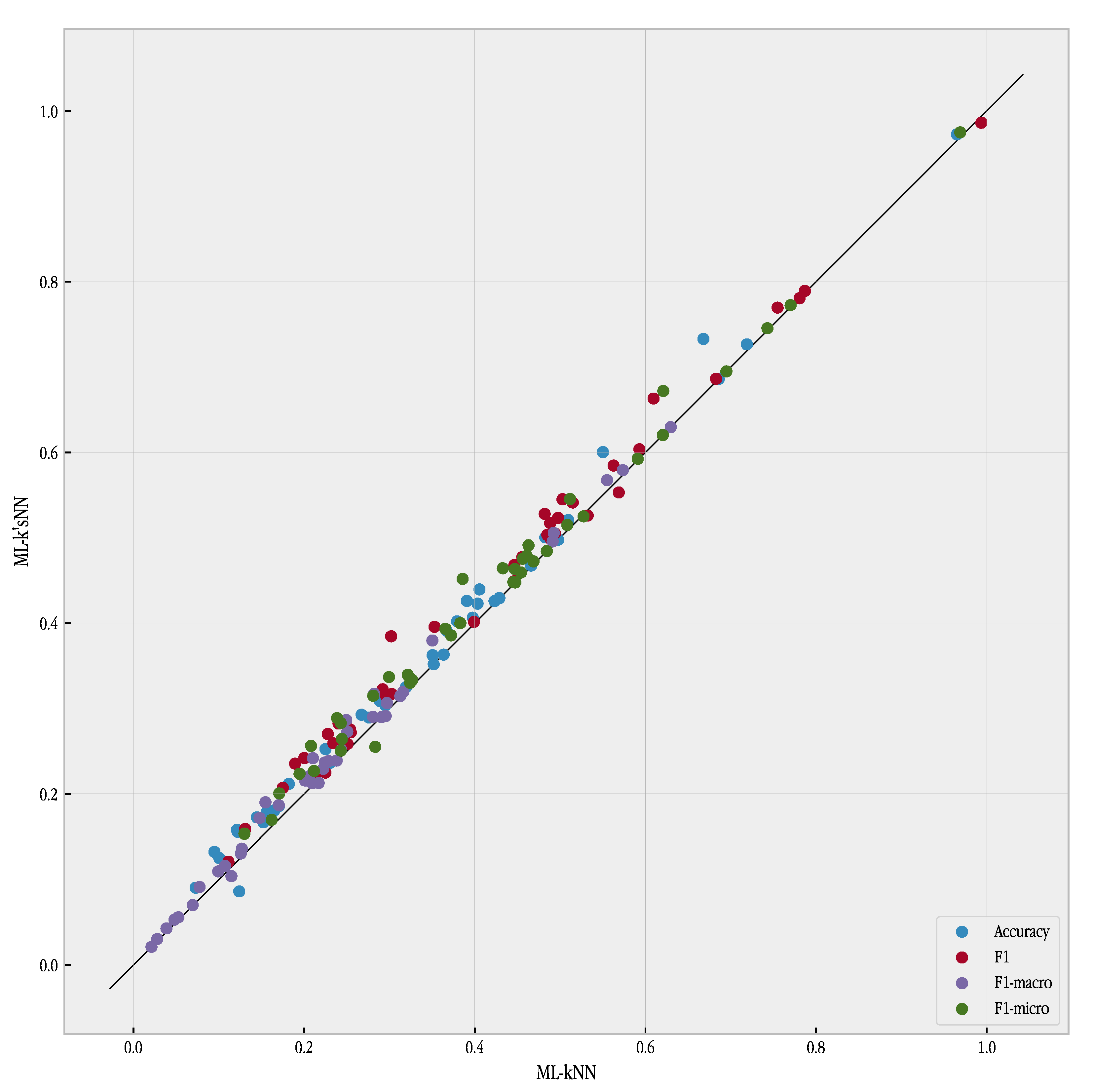
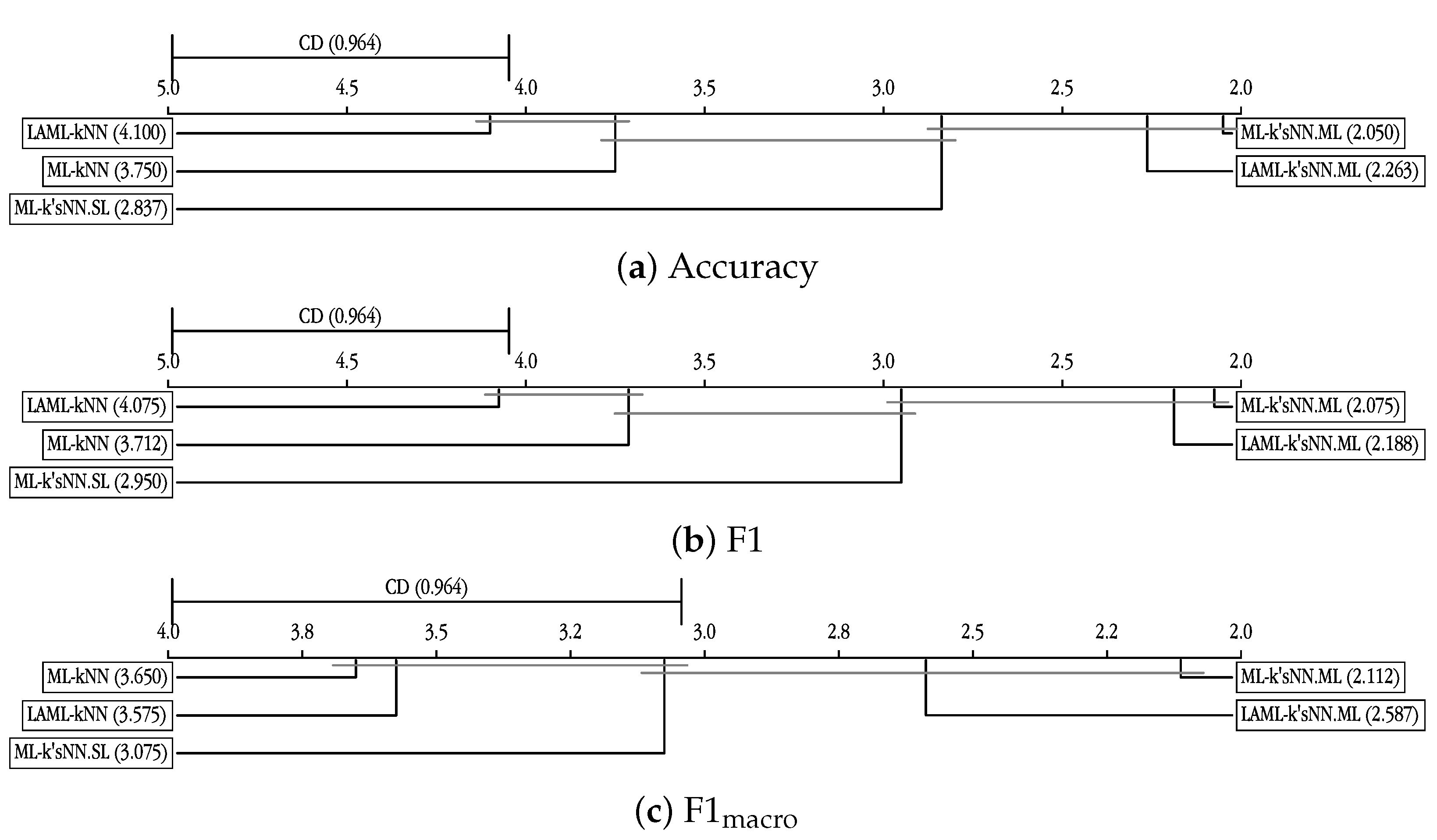
Individual results for each dataset are shown in Figure 1. This figure represents the results for every datasets of ML-kNN and ML-k’sNN. Points above the main diagonal correspond to problems where our method outperformed ML-kNN. It can be seen in the figure that almost all points indicate a better performance of ML-k’sNN. Figure 2 shows the Nemenyi test for those same metrics using a graph representation [34]. In this plot, we show the critical difference, CD. Then we show for every algorithm its average rank, $R_j$. Two algorithms i and j can be considered significantly different if $|R_i-R_j|>CD$. In order to show that information, a horizontal line connects all groups of algorithms that do not fulfill that condition and should be considered as performing equally. Iman–Davenport tests for all four metrics obtained a p-value of 0.0000.

The first metric studied was accuracy. Table 2 shows the comparison using the Wilcoxon test for the five studied methods and Figure a illustrates the Nemenyi test. The first piece of information we obtain from the Figure is that the methods are sorted from best (left hand side of the figure) to worst (right hand side) according to average ranks. This average rank is by itself a good indicator of the performance of any model. The second piece of information is given by the critical difference (CD = 0.964). If two methods’ ranks differ more than 0.964 then Nemenyi test result tells us that there are significant differences in their performance. That is the reason why the methods whose ranks are below that difference are linked with a horizontal line. Thus, according to the Nemenyi test, the single-label ML-k’sNN approach was able to significantly improve standard ML-kNN. Although it achieved a better average rank, the Nemenyi test did not find significant differences. However, the Wilcoxon test found significant differences between ML-kNN and ML-k’sNN.SL. A further study of the results showed that this approach tended to exhibit over-learning. It was the best method in terms of training performance, but its performance was worse in terms of testing accuracy. This behavior of ML-k’sNN.SL was reproduced for all the remaining metrics. ML-k’sNN.ML demonstrated better performance than ML-kNN, according to both tests. This method had a clear advantage over the standard approach, improving the results of ML-kNN for 35 of the 40 datasets. ML-k’sNN.ML and LAML-k’sNN.ML improved the two studied versions of ML-kNN.

Table 3 shows the comparison for F1 metric. For this metric, our proposed method obtained very good results. The two studied versions of ML-k’sNN based on the multi-label approach outperformed both versions of ML-kNN. The differences are significant in all cases and for both tests, Wilcoxon and Nemenyi. ML-k’sNN.SL improved the results of ML-kNN according to the Wilcoxon test, although the Nemenyi test failed to find significant differences. The improvement of LAML-k’sNN.ML with respect to LAML-kNN is remarkable.

We also carried out experiments for macro- and micro-averaged versions of the F1 metric. The results of the comparisons are shown in Table 4 and Table 5, respectively. Iman–Davenport tests for all three metrics obtained a p-value of 0.000. For these two metrics, ML-k’sNN.ML and LAML-k’sNN.ML improved the results for the standard versions ML-kNN and LAML-kNN. ML-k’sNN.SL achieved a better average rank than ML-kNN, but without significant differences, according all the tests.

Our second set of experiments was devoted to ranking metrics. The results for the tests are shown in

Table 6. Comparison of the different methods using average precision metric.

		ML-kNN	ML-k’sNN.EC	LAML-kNN	LAML-k’sNN.EC	ML-k’sNN.SL
Mean		0.5070	0.5341	0.4970	0.5338	0.5014
Ranks		3.2375	1.8750	3.8625	2.3500	3.6750
	w/l		32/8	12/19	25/15	16/24
ML-kNN	p		0.0000	0.0837	0.0007	0.3134
	$R^{+}/R^{-}$		750.0/70.0	281.5/538.5	662.0/158.0	335.0/485.0
	w/l			5/35	15/25	7/33
ML-k’sNN.EC	p			0.0000	0.3007	0.0000
	$R^{+}/R^{-}$			65.0/755.0	333.0/487.0	59.0/761.0
	w/l				32/8	24/16
LAML-kNN	p				0.0000	0.2763
	$R^{+}/R^{-}$				769.0/51.0	491.0/329.0
	w/l					6/34
LAML-k’sNN.EC	p					0.0000
	$R^{+}/R^{-}$					61.0/759.0

,

Table 7. Comparison of the different methods using coverage metric.

		ML-kNN	ML-k’sNN.EC	LAML-kNN	LAML-k’sNN.EC	ML-k’sNN.SL
Mean		29.8870	25.3049	27.3205	27.4480	36.7408
Ranks		3.1000	2.0125	3.5500	2.3875	B
	w/l		28/12	8/22	26/14	17/23
ML-kNN	p		0.0008	0.0286	0.0372	0.0294
	$R^{+}/R^{-}$		659.0/161.0	247.5/572.5	565.0/255.0	248.0/572.0
	w/l			9/30	14/26	5/35
ML-k’sNN.EC	p			0.0016	0.2016	0.0000
	$R^{+}/R^{-}$			175.5/644.5	315.0/505.0	87.0/733.0
	w/l				30/9	14/26
LAML-kNN	p				0.0204	0.0061
	$R^{+}/R^{-}$				582.5/237.5	206.0/614.0
	w/l					6/34
LAML-k’sNN.EC	p					0.0000
	$R^{+}/R^{-}$					82.0/738.0

and

Table 8. Comparison of the different methods using ranking loss metric.

		ML-kNN	ML-k’sNN.EC	LAML-kNN	LAML-k’sNN.EC	ML-k’sNN.SL
Mean		0.1099	0.0827	0.1095	0.1256	0.1101
Ranks		2.9375	1.8375	3.3250	3.5875	3.3125
	w/l		33/7	10/16	14/26	13/26
ML-kNN	p		0.0003	0.3408	0.0983	0.3232
	$R^{+}/R^{-}$		676.0/144.0	339.5/480.5	287.0/533.0	336.5/483.5
	w/l			7/33	8/31	11/29
ML-k’sNN.EC	p			0.0002	0.0001	0.0050
	$R^{+}/R^{-}$			130.0/690.0	111.5/708.5	201.0/619.0
	w/l				17/23	19/19
LAML-kNN	p				0.2369	0.8350
	$R^{+}/R^{-}$				322.0/498.0	394.5/425.5
	w/l					23/17
LAML-k’sNN.EC	p					0.2264
	$R^{+}/R^{-}$					500.0/320.0

for average precision, ranking loss and coverage, respectively. Figure 3 illustrates the results for ML-kNN and ML-k’sNN for the same three metrics. To obtain a homogeneous plot, ranking loss is represented as 1-“ranking loss” and coverage is represented as the relative coverage with respect to the optimal value. In that way, all the points above the main diagonal demonstrate the superior performance of our proposal. Nemenyi test results are shown in Figure 4.

As explained above, an evolutionary computation method was used to obtain the optimal k values when the ranking metrics needed to be optimized. The single-label version of our method, ML-k’sNN.SL, demonstrated poor performance for the three ranking metrics. This was not an unexpected result, as this method does not consider any kind of multi-label information. On the other hand, ML-k’sNN.EC achieved remarkably good performance. For all three metrics, it improved the results of the standard version, according to both the Wilcoxon and Nemenyi tests. LAML-k’sNN.EC improved the results of LAML-kNN for average precision and coverage. However, ranking loss obtained a worse average ranking, although the differences were not significant.

In order to gain a deeper understanding of our proposal, we studied the average value of the obtained k’s for all the labels. Figure 5a shows this average value when the datasets are sorted according to the number of features. The average values exhibited a tendency toward larger values for datasets with less features. It is also interesting to point out that, although the values for the different labels in ML-k’sNN.ML show a large variation, the averaged values were very similar to the best value obtained for ML-kNN through cross-validation, as it shown in the figure. ML-k’sNN.SL obtained systematically smaller values of k, due to the fact that, for its single-label approach, $k=1$ was often the best value.

Both LAML-kNN and LAML-k’sNN obtained smaller values than ML-kNN and ML-k’sNN. As the former two methods work with smaller clusters, it is expected that the optimal k within each cluster would be smaller.

Figure 5b shows the same average value of k when the datasets are sorted according to the number of labels. Interestingly, ML-kNN and ML-k’sNN.ML obtained larger values when the number of labels was small or large, and lower values for the datasets with a medium number of labels.

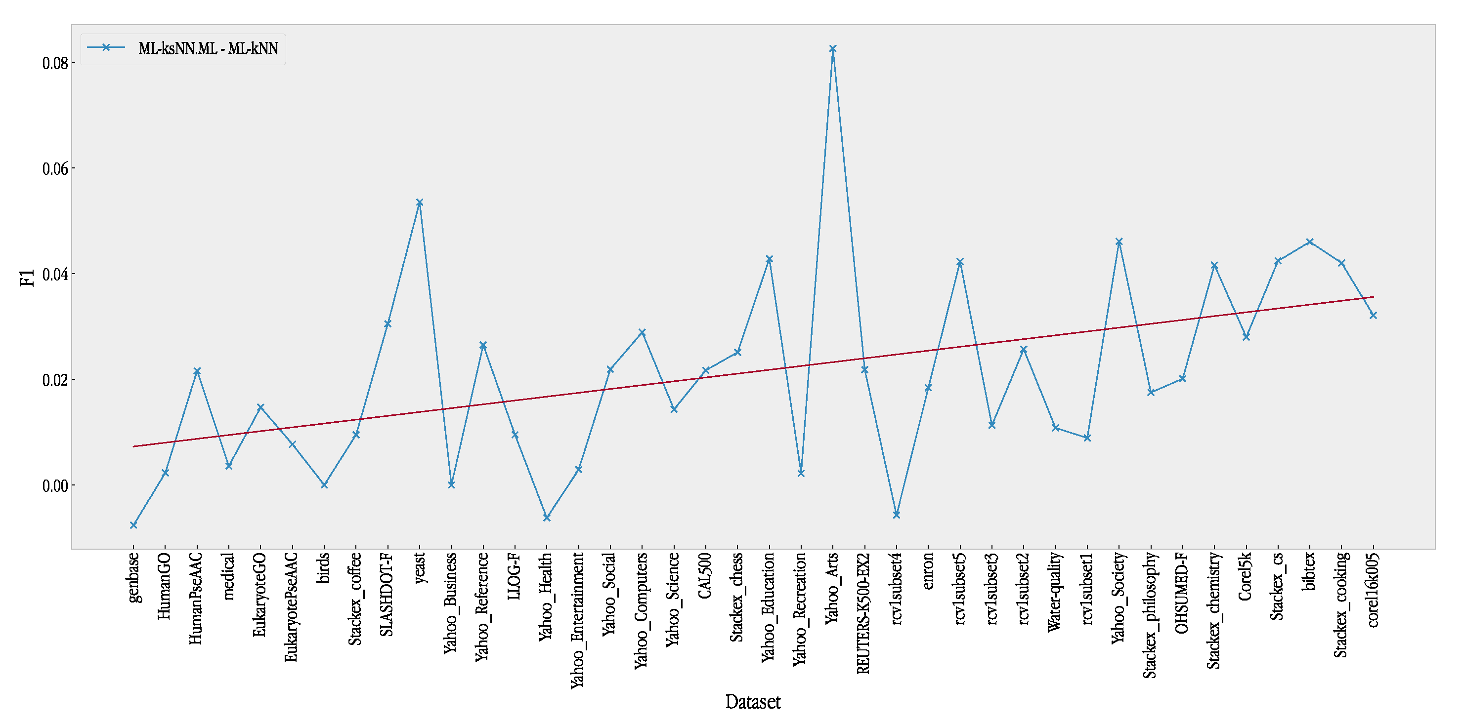
Another interesting issue is the relative behavior of ML-k’sNN with respect to ML-kNN, depending on the characteristic of the datasets. This is always a very difficult task, as most algorithms do not show a clear trend of behavior in regard to particular characteristics of the datasets. We studied the performance of the standard method and our approach regarding the diversity of the datasets. Figure 6 shows the difference in performance using the F1 metric between ML-k’sNN and ML-kNN when the datasets are sorted in terms of increasing diversity.

The figure displays a tendency of ML-k’sNN to improve its relative performance when the diversity of the datasets increases. To obtain a clearer idea of the general trend of the differences, the figure shows a linear regression of the difference in terms of the F1 metric. Thus, linear regression has a clear upward slope. This an interesting property of our proposal, as datasets with higher diversity are usually more difficult to address. A similar study that considered the number of labels was carried out (see Figure 7). Again, our proposed method demonstrated better behavior as the number of labels increased. These two figures shows that ML-k’sNN is more effective when the multi-label problem is more difficult, i.e., when there are many labels and many diverse sets of relevant labels.

5.1. Comparison with Other Instance-Based Learning Methods

In the previous section we have shown that our algorithm was able to beat the standard ML-kNN algorithm and another version of that algorithm, LAML-kNN. However, other modifications of ML-kNN have been proposed in the literature. In this section we present a comparison with several versions of ML-kNN and other instance-based methods. We compared the best version of our proposal, ML-k’sNN.ML for classification metrics and ML-k’sNN.EC for ranking metrics, with ML-kNN, LAML-kNN, two binary relevance implementations of k-NN in scikit learn Python package [40], BRkNNa and BRkNNb, stacked ML-kNN [41] (SMLkNN), dependent ML-kNN (DMLkNN) [22], soft relevance for multi-label classification [25] (Mr.KNN), the combination of instance-based learning and logistic regression for multilabel classification, IBLR-ML and IBLR-ML+ [42], and a recent method for obtaining local k values for ML-kNN, ML-localkNN [43]. 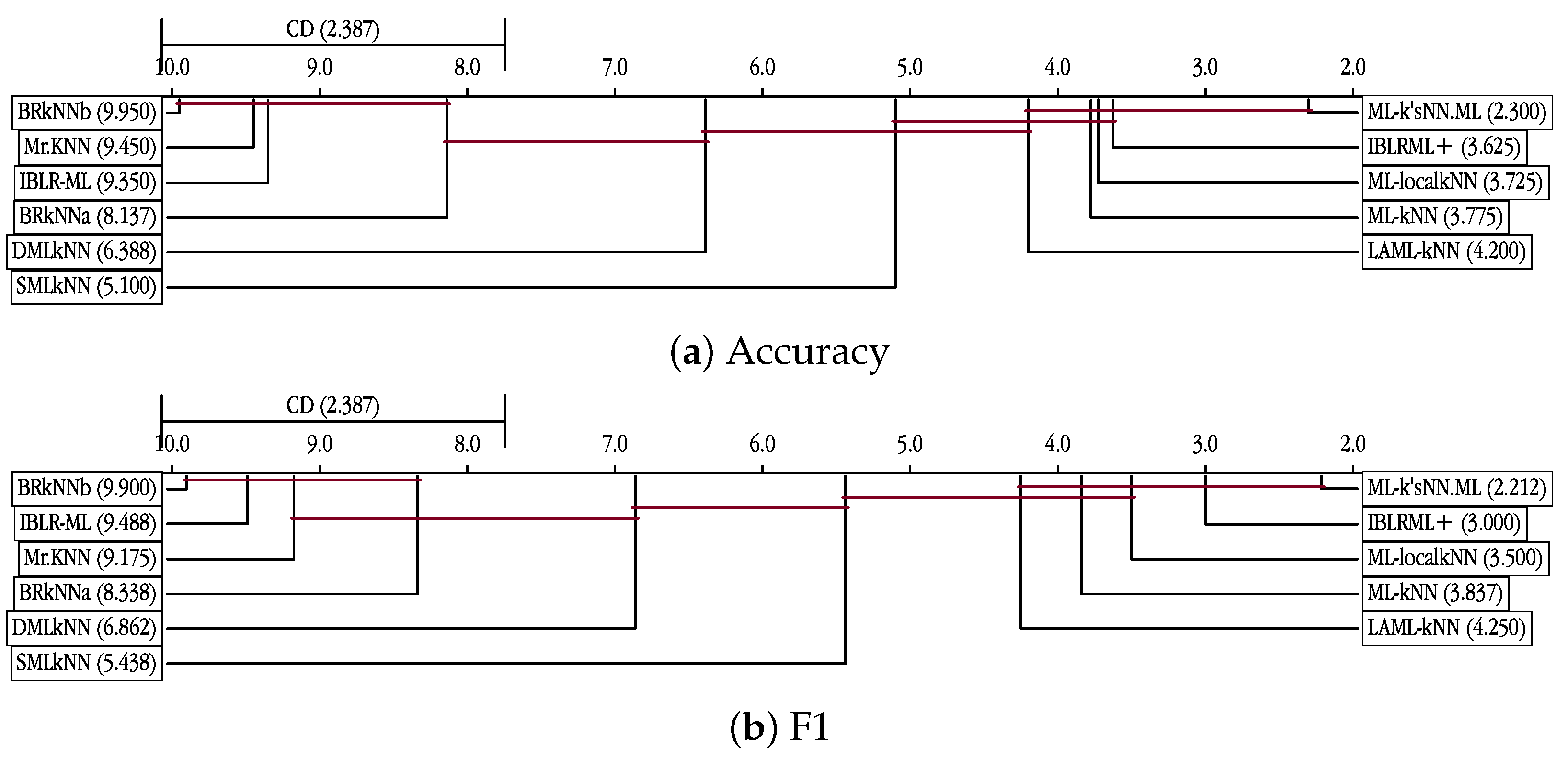Figure 8 and Figure 9 show the Nemenyi test for classification and ranking metrics, respectively. BRkNNa and BRkNNb are not implemented for ranking metrics so they are not shown in Figure 9. The Iman–Davenport test found significant differences for all seven metrics.

The first interesting result was that, in general, none of the modifications of ML-kNN showed a consistently better performance than the original proposal with the exception of ML-localkNN and IBLRML+. The second interesting result was that our proposal always achieved the best performance in terms of the average ranking regardless of the metric considered. Nemenyi test found significant differences most of the times. These differences are specially marked for ranking metrics.

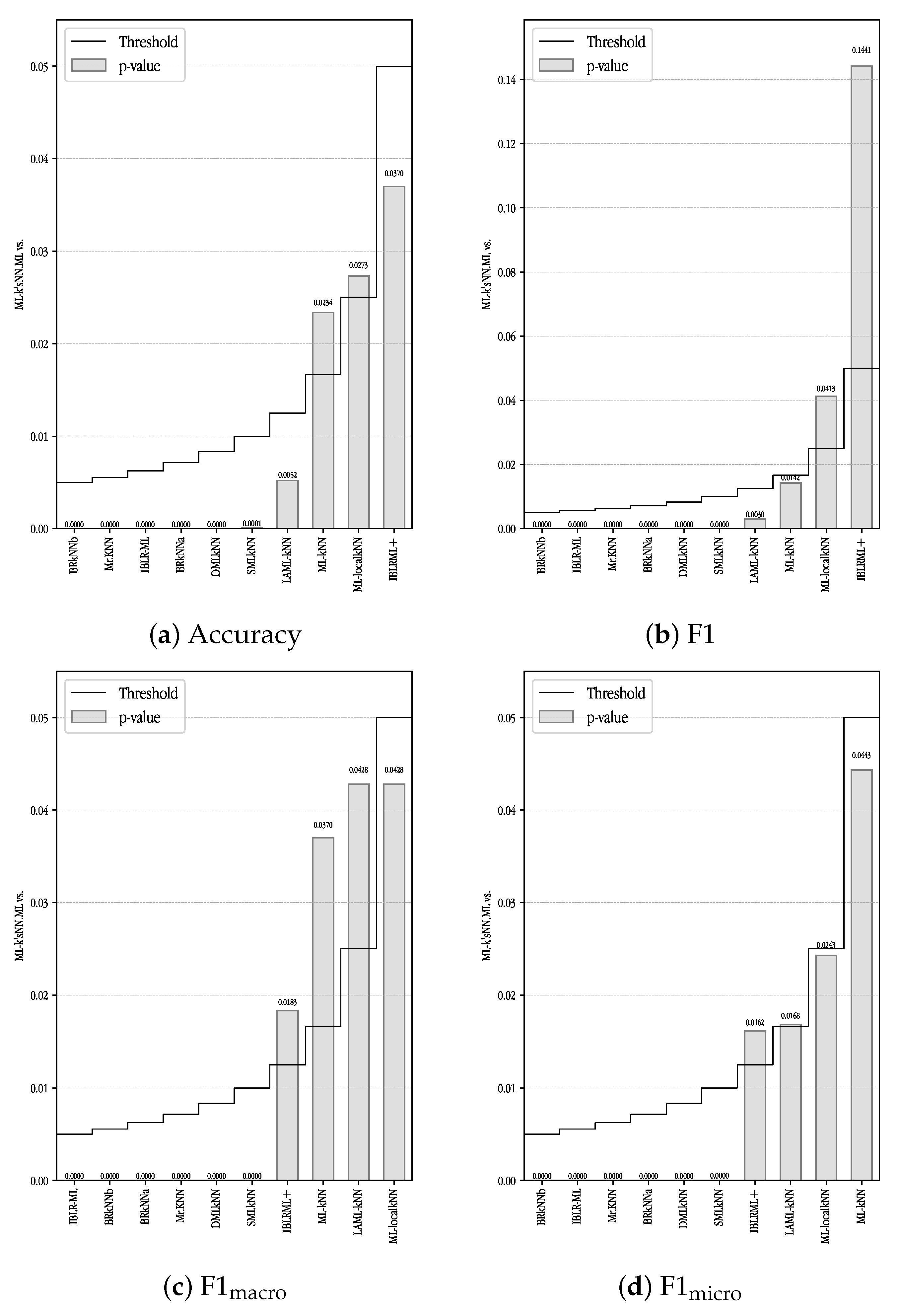
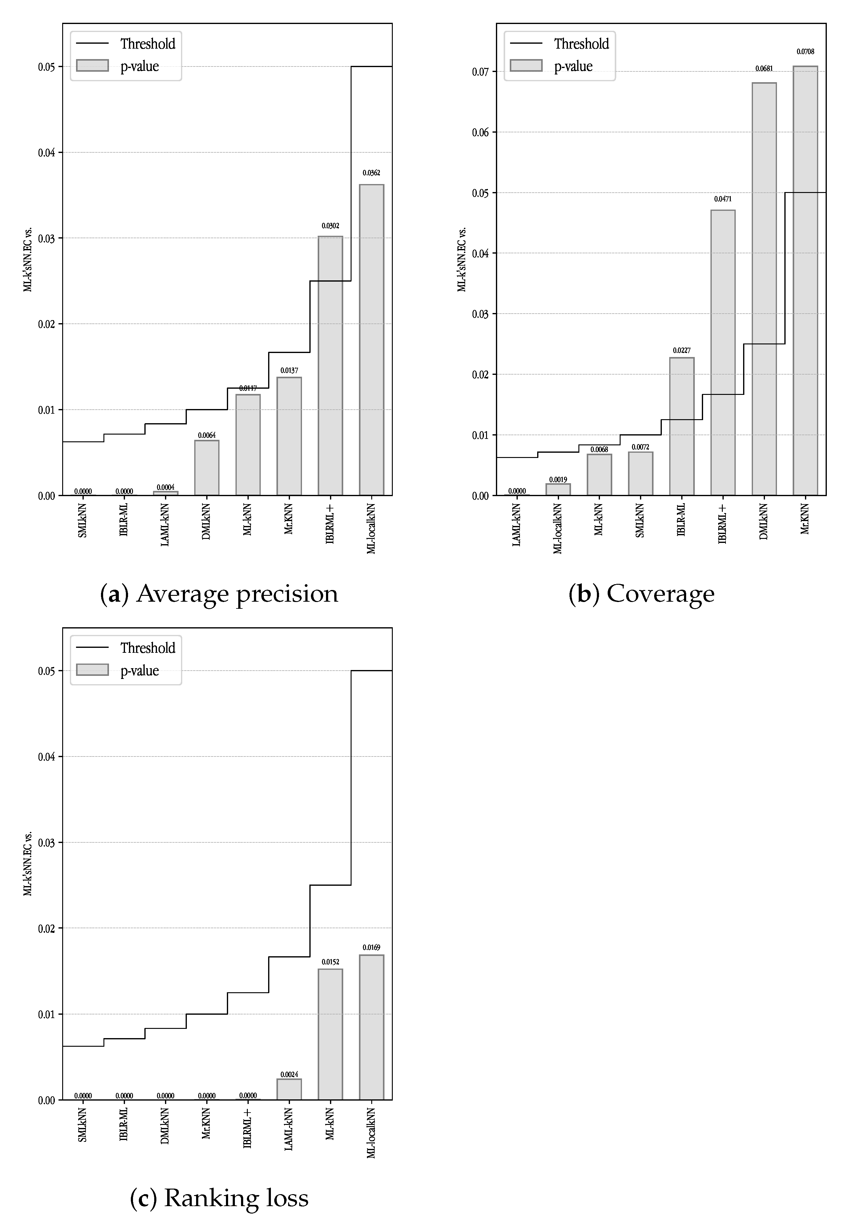
After applying the Iman–Davenport test, we carry out a Holm’s procedure [34] for controlling the family wise error in multiple hypothesis testing. In Holm’s procedure, the best-performing algorithm in terms of Friedman’s ranks is compared in a stepwise manner against the other methods. We carried out this procedure for the seven metrics. Figure 10 and Figure 11 show a graphical representation of Holm test for classification and ranking metrics, respectively. The methods are shown in increasing values of average ranks and a bar plot shows the p-value of the statistical test. A horizontal line shows the critical value of the test. Bars below this horizontal lines mean a significant difference.

In Figure 10 we can see the good performance of ML-k’sNN. For the four classification metrics it was able to significantly improve the remaining methods. For accuracy it showed a significantly better performance than 7 of the 10 methods used for the comparison. For F1, only ML-localkNN and IBLRML+ were not worse than ML-k’sNN. For F1${}_{\mathrm{macro}}$ and F1${}_{\mathrm{micro}}$, ML-k’sNN beat 6 of the 10 methods. As we cannot expect any algorithm to be always the best performing one for every dataset and metric, the fact that MLk’sNN was able to obtain the overall best results for the four metrics is remarkable. Furthermore, we must take into account that most of these methods can also use our proposal to be improved.

For ranking metrics—see Figure 11—the performance of ML-k’sNN was even better. For averaged precision it was better than all the methods with the exception of IBLRML+ and ML-localkNN. For ranking loss it improved the results of all the methods. For coverage it also achieved the best results but the differences were not significant against the four best performing methods.

5.2. Instance Selection

Instance selection is a widely used method in single-label classification that improves the performance of instance-based methods and reduces the size of the training set [44]. For single-label problems, evolutionary algorithms have demonstrated better performance and also a good scalability [45,46]. For multi-label datasets, only a few methods have been developed [47,48,49,50,51].

An interesting aspect of this work is the study of whether our approach is able to maintain its superior performance when instance selection is applied [52,53]. As we are not proposing a new instance selection algorithm, we used for both the standard ML-kNN method and ML-k’sNN a very simple CHC evolutionary computational approach [54,55] which has proven its efficiency for instance selection in single-label problems [56].

We used populations of 100 individuals evolved for 1000 generations. This experiment was carried out using the F1 metric.

Table 9. Comparison of the different methods’ instance selection results.

F1 Metric
		ML-kNN	ML-k’sNN	LAML-kNN	LAML-k’sNN
Mean		0.3472	0.3803	0.3000	0.3729
Ranks		2.4625	1.8875	3.7000	1.9500
	w/l		25/10	4/36	27/13
ML-kNN	p		0.0006	0.0000	0.1789
	$R^{+}/R^{-}$		664.5/155.5	91.0/729.0	510.0/310.0
	w/l			2/38	21/19
ML-k’sNN	p			0.0000	0.9250
	$R^{+}/R^{-}$			5.0/815.0	403.0/417.0
	w/l				34/6
LAML-kNN	p				0.0000
	$R^{+}/R^{-}$				724.0/96.0
Reduction
		ML-kNN	ML-k’sNN	LAML-kNN	LAML-k’sNN
Mean		0.9400	0.9558	0.9573	0.9424
Ranks		3.0875	2.0500	2.1000	2.7625
	w/l		30/9	28/12	25/15
ML-kNN	p		0.0004	0.0002	0.2589
	$R^{+}/R^{-}$		675.5/144.5	686.0/134.0	494.0/326.0
	w/l			18/21	14/26
ML-k’sNN	p			0.8350	0.0360
	$R^{+}/R^{-}$			425.5/394.5	254.0/566.0
	w/l				10/29
LAML-kNN	p				0.0001
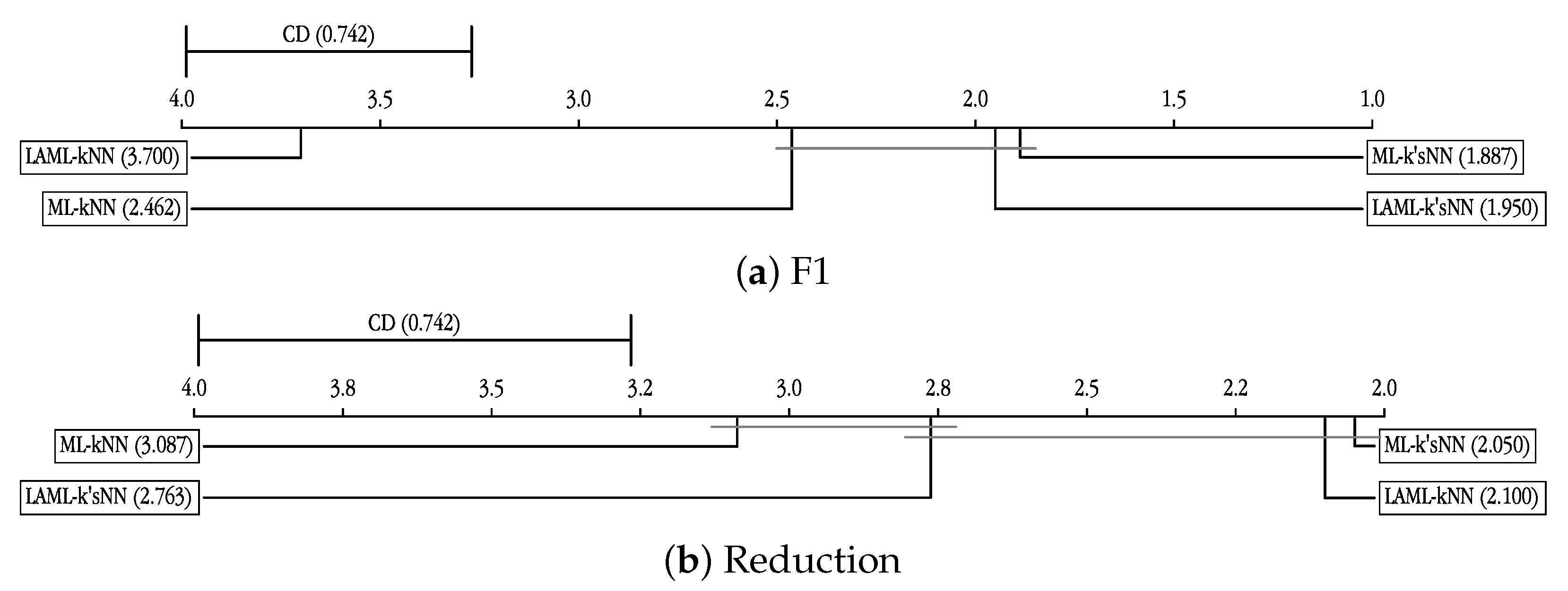
	$R^{+}/R^{-}$				108.5/711.5

shows the comparison among the different methods in terms of the F1 metric and reduction. Comparisons in terms of the Nemenyi test are shown in Figure 12.

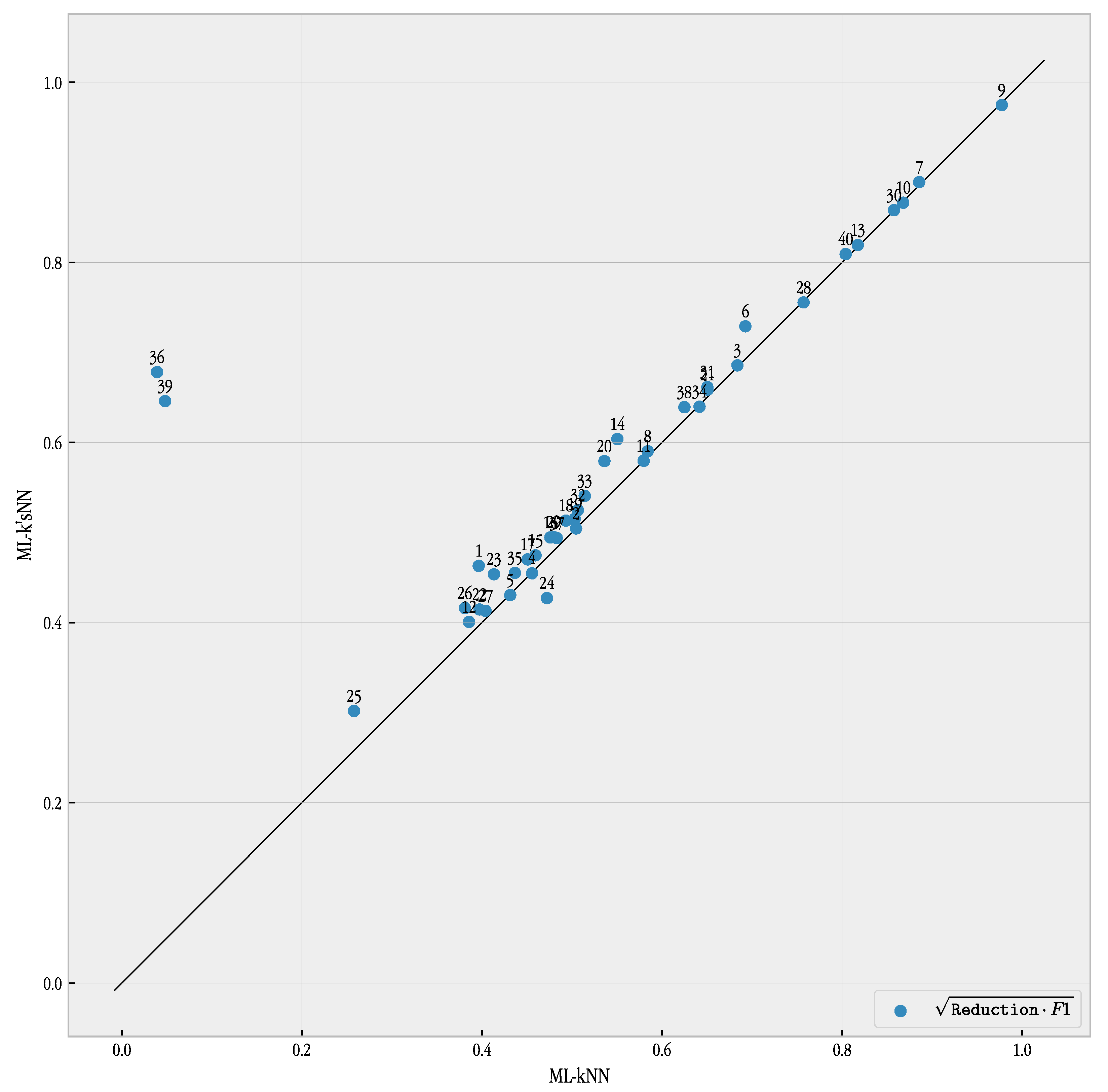
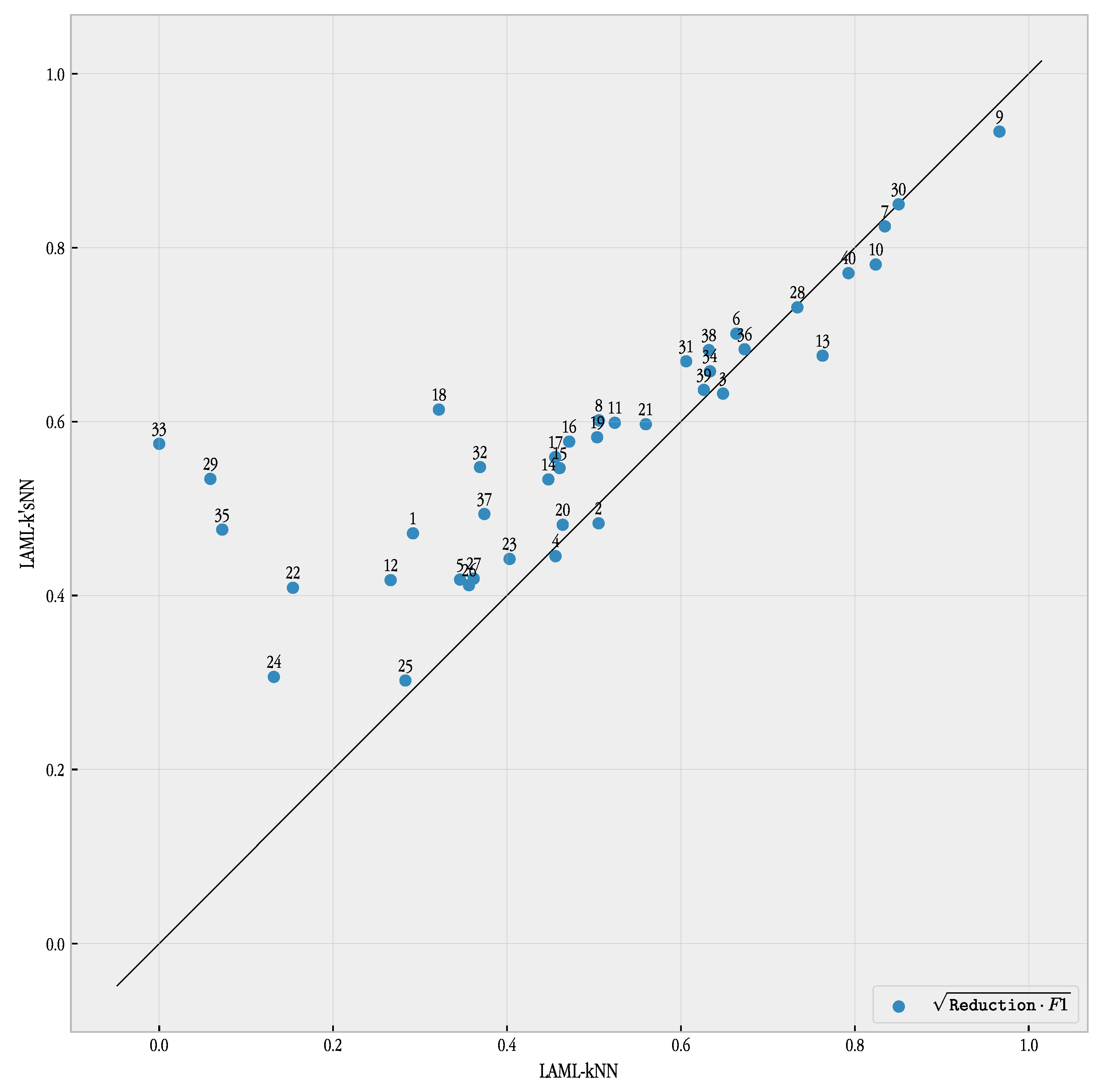
Regarding the comparison between ML-kNN and ML-k’sNN, the tables demonstrate the superior performance of our proposed method. ML-k’sNN achieved better results in both reduction and the F1 metric. These differences were significant, according to the Wilcoxon test. This behavior is illustrated in Figure 13, where the results of the geometric mean of F1 and reduction are plotted for both ML-kNN and ML-k’sNN. With the exception of dataset #24, Stackex_coffee, the combined performance of reduction and F1 is always better for ML-k’sNN.

The comparison with LAML-kNN showed different results. LAML-k’sNN improved the F1 metric performance of LAML-kNN but with a lower level of reduction. However, the combined reduction and F1 metric performance—see Figure 14—was very favorable to our proposed method. In most cases, the differences in performance are rather large, and the performance of LAML-k’sNN is clearly superior.

6. Conclusions

In this paper, we have proposed a new multi-label classification algorithm, ML-k’sNN, based on the ML-kNN algorithm in which different values of k are used for each label. Three different methods for obtaining the set of k’s for every label are proposed and tested. Depending on the metric to be optimized, a label independent or evolutionary approach are used. The complexity of the three approached varies, so choosing the best one for a specific task would depend on the available resources and performance constraints.

The proposed method is studied using two different implementations of ML-kNN, the standard ML-kNN method and the locally adaptive ML-kNN method, LAML-kNN. However, the proposed method can be applied to almost any other version of ML-kNN. Using a large set of 40 problems with different characteristics, our proposed method demonstrated better performance when compared to both ML-kNN implementations. A further study has shown that our proposed method was able to improve, as a general rule, its performance when there are more labels in the dataset or when the diversity of the labels increases, although for some datasets it might not be the case. Furthermore, the improvement demonstrated by ML-k’sNN was maintained when the method was coupled with instance selection. In fact, the good performance of our approach was kept while obtaining a large reduction in training set size.

A final experiment compared our algorithm with ten different ML-kNN variants. This comparison showed the overall best performance of ML-k’sNN for all the four classification metrics and the three ranking metrics.

A promising research line is extending our approach to other methods based on ML-kNN. Almost any variant of ML-kNN, such as the used in the experiments, can be adapted to work with a k more appropriate for every label. In this way, our proposal may benefit other variants of instance-based multi-label learning methods.