Learning Wasserstein Contrastive Color Histogram Representation for Low-Light Image Enhancement

Abstract

The goal of low-light image enhancement (LLIE) is to enhance perception to restore normal-light images. The primary emphasis of earlier LLIE methods was on enhancing the illumination while paying less attention to the color distortions and noise in the dark. In comparison to the ground truth, the restored images frequently exhibit inconsistent color and residual noise. To this end, this paper introduces a Wasserstein contrastive regularization method (WCR) for LLIE. The WCR regularizes the color histogram (CH) representation of the restored image to keep its color consistency while removing noise. Specifically, the WCR contains two novel designs including a differentiable CH module (DCHM) and a WCR loss. The DCHM serves as a modular component that can be easily integrated into the network to enable end-to-end learning of the image CH. Afterwards, to ensure color consistency, we utilize the Wasserstein distance (WD) to quantify the resemblance of the learnable CHs between the restored image and the normal-light image. Then, the regularized WD is used to construct the WCR loss, which is a triplet loss and takes the normal-light images as positive samples, the low-light images as negative samples, and the restored images as anchor samples. The WCR loss pulls the anchor samples closer to the positive samples and simultaneously pushes them away from the negative samples so as to help the anchors remove the noise in the dark. Notably, the proposed WCR method was only used for training, and was shown to achieve high performance and high speed inference using lightweight networks. Therefore, it is valuable for real-time applications such as night automatic driving and night reversing image enhancement. Extensive evaluations on benchmark datasets such as LOL, FiveK, and UIEB showed that the proposed WCR method achieves superior performance, outperforming existing state-of-the-art methods.

1. Introduction

Low-light images captured in natural scenes under insufficient illumination conditions often suffer from unpleasing visual perceptions, including low contrast and visibility, unpleasing color distortions, and noise. Besides these issues, the degradations are adverse to a variety of high-level computer vision tasks, including, but not limited to, video surveillance [1], depth estimation [2], and face detection [3,4].

In recent decades, there has been a growing interest in low-light image enhancement (LLIE) [5,6,7,8,9], which focuses on enhancing the illumination to restore normal-light images. Most of the traditional LLIE methods are based on histogram equalization (HE) [10] and Retinex theory [11,12]. The traditional methods have achieved good performance on specific images and have also inspired recent work [13,14]. However, these methods focus on modifying the intensity values of pixels, but cannot automatically learn the effective image feature representations that can fully describe the natural image intrinsic characteristics, resulting in unnatural enhancement such as lost details and distorted colors.

To further advance LLIE, deep learning [15] has been introduced into LLIE, which can automatically learn effective feature representations from a large amount of images in an end-to-end manner.

In spite of proven achievements, most deep learning-based LLIE methods [5,6,7,15,16,17,18,19] suffer from the issue of color inconsistency or residual noise. First, to guide the training of the model, they adopt pixel-wise loss, such as L1/L2-based image reconstruction loss, which cannot capture global color statistics (e.g., mean and variance) differences, leading to color inconsistency between the restored images and the normal-light images (see Figure 1c–e).

For instance, if we take a color image and shift it by one pixel, the resulting shifted image will exhibit nearly identical color statistics to the original image, but their pixel-wise loss may indicate significant differences between them. Second, such approaches, including state-of-the-art KinD++ [5] and DCCNet [7], only regard well-exposed normal-light images as supervisory signals, neglecting to model the noise present in the low-light images. As depicted in Figure 1c,d, this may cause the restored image to suffer from severe residual noise, leading to unpleasing visual effects.

In this research, we present a naval Wasserstein contrastive regularization method (WCR) for LLIE to address the aforementioned problems, which can effectively regularize the CH representation of the restored image to maintain its color consistency while removing noise. Specifically, the proposed WCR comprises two components: a differentiable CH module (DCHM) and a WCR loss. To learn the CH representation, the DCHM combines low-light images, their matching restored images, and the normal-light images into a color space. Subsequently, we lift the DCH to Wasserstein space, where the distance stands in for the expense of the most efficient transfer of a complete color distribution between two locations. Inspired by contrastive learning (CL) [21,22], we further formulate the WCR loss as a triplet loss, which pulls the restored images closer to the normal-light images while pushing the restored images farther away from the low-light images in Wasserstein space. The proposed WCR method was evaluated through comprehensive experiments on three widely used benchmark datasets, namely, LOL [13], FiveK [23], and UIEB [24]. The results clearly indicate the proficiency of WCR on keeping color consistency and removing residual noise.

In conclusion, this work offers the following main contributions:

• A novel WCR framework is proposed for LLIE, which regularizes the CH representation of the restored image in Wasserstein space to keep its color consistency while removing residual noise;
• A DCHM was designed that can be readily injected into the network to learn the image CH representation in an end-to-end mode;
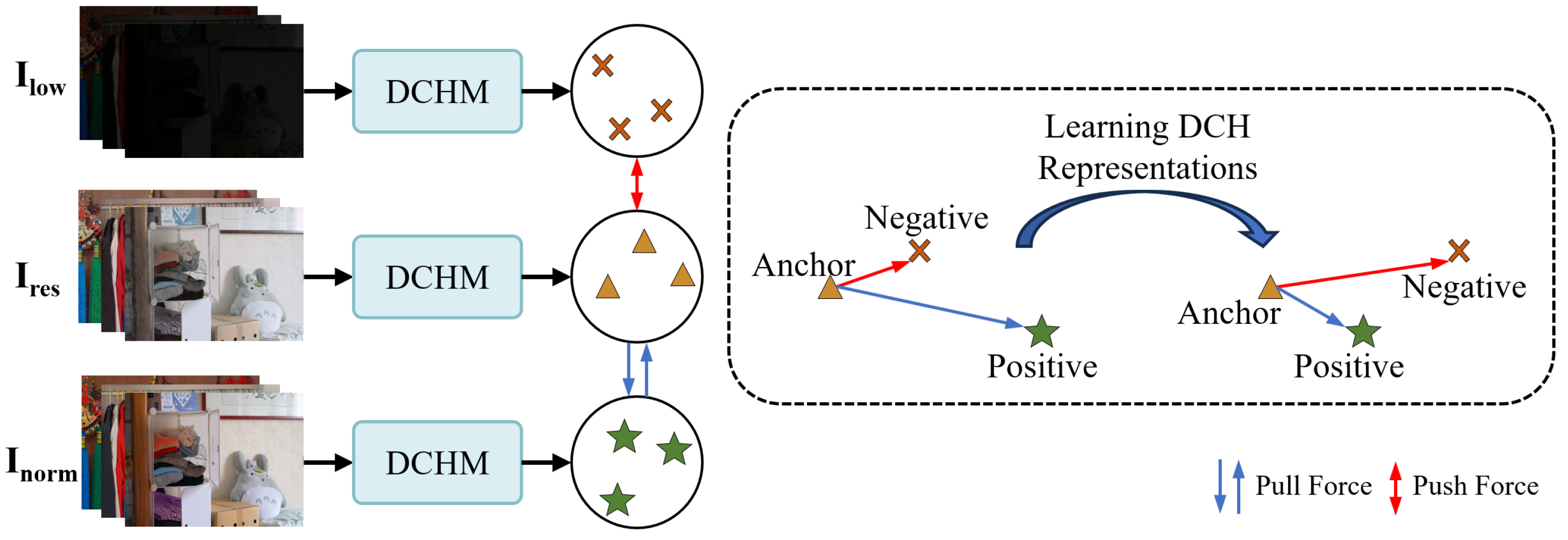
• We constructed a WCR loss that introduces low-light images as negative samples for CL, which effectively reduces the residual noise.

The rest of the paper is organized as follows. Section 2 presents an overview of the related works. Section 3 delves into the specifics of our proposed WCR method. Section 4 contains the experimental results and analyses conducted on three datasets: LOL [13], MIT FiveK [23], and UIEB [24]. Then, the discussion is presented in Section 5. Finally, we outline the conclusions in Section 6.

2. Related Work

2.1. Low-Light Image Enhancement

LLIE is a long-standing research topic and various approaches have been proposed. These can be categorized into two classes: traditional LLIE [10,11,12] and deep learning-based LLIE [5,6,7,19,25,26].

Traditional LLIE. HE-based approaches [10] and Retinex theory-based methods [11,12] are two main categories that can be used to categorize early LLIE methods. The HE can improve the visibility of dark images by increasing the dynamic range. However, the HE is primarily designed to enhance contrast rather than adjust illumination, and as a result, it tends to be sensitive to noise in low-light images. Similarly, the Retinex theory hypothesis presupposes that an image is made up of both illumination and reflection, yet it can provide exaggerated enhancements like lost features and color distortions. In addition, the Retinex model typically does not account for noise, leading to a large amount of noise during the enhancement process.

Deep learning-based LLIE. Deep learning has become increasingly popular in the field of LLIE due to its capabilities in end-to-end learning. LLNet [19], a pioneering work in this field, tackles the LLIE problem using stacked sparse denoising autoencoders. MBLLEN [25] is a pioneering research that introduces LLIE algorithms to video processing, while KinD [27] and KinD++ [5] are data-driven approaches that leverage Retinex theory to alleviate issues related to illumination adjustment and the removal of artifacts in the LLIE. Additionally, Zero-DCE [28] and Zero-DCE++ [29] use curve estimation to achieve zero-reference image illumination enhancement. In a different approach, SCI [30] develops a new self-calibrating illumination learning framework for achieving fast image brightening in low-light conditions in the real world. Another work by Wu et al. [14] expands an optimization problem into a learnable network to decompose low-light images into reflectance and illumination layers, achieving noise suppression and detail preservation in the final decomposition results. DCCNet [7] learns the color distribution and grayscale content separately from the input, and then fuses them through a pyramid color embedding module to obtain the restored image. Normalization flow is employed by Zhang et al. [16] to improve stability in the context of low-light video enhancement. Similarly, LLFlow [6] utilizes normalizing flow techniques to handle illumination adjustment and noise suppression in low-light scenarios. Despite the demonstrated promising results, the above methods tend to suffer from the issue of color inconsistency or residual noise. For example, KinD++ [5] performs multiscale reconstruction of illumination and reflection based on Retinex, ignoring the learning of color and noise representations. DCCNet [7] directly predicts the color representation of normal-light images with low light-images, resulting in a significant amount of residual noise. LLFlow [6], conditioned on low-light images, learns a reversible network that transforms the distribution of normal-light images into a Gaussian distribution. While it effectively eliminates noise, the oversmoothing effect can lead to color distortions.

2.2. Contrastive Learning

CL [21,22] has gained significant popularity as a representation learning paradigm in the realm of computer vision. By contrasting positive pairs with negative pairs, the CL approach allows for representation learning, which is frequently used in various high-level computer vision tasks, including image classification [22], object detection [31,32], and image segmentation [33].

Over the last few years, there have been some attempts to investigate the utilization of CL in lower-level tasks [34,35,36,37]. Wu et al. [34] even demonstrate that CL can be very effective in improving image dehazing. Semi-UIR [35] uses a mean teacher-based semisupervised underwater image restoration framework, which incorporates contrastive regularization to mitigate the overfitting caused by incorrect labels. SCL-LLE [36] leverages CL for LLIE that allows the LLIE model to use both positive and negative samples, and uses the scene semantics to regularize the image enhancement network. Fu et al. [37] introduce the regularizer-free Retinex decomposition and synthesis network, which incorporates CL to impose constraints on Retinex decomposition. Typically, these methods result in color deviations because they neglect the global color statistics of the image, which can be effectively captured by the CH representation learned through the proposed DCHM.

3. Methodology

We first provide a summary of the proposed WCR framework for LLIE in Section 3.1. Then, we provide details of the WCR method, which contains two key designs including a DCHM (Section 3.2) and a WCR loss (Section 3.3).

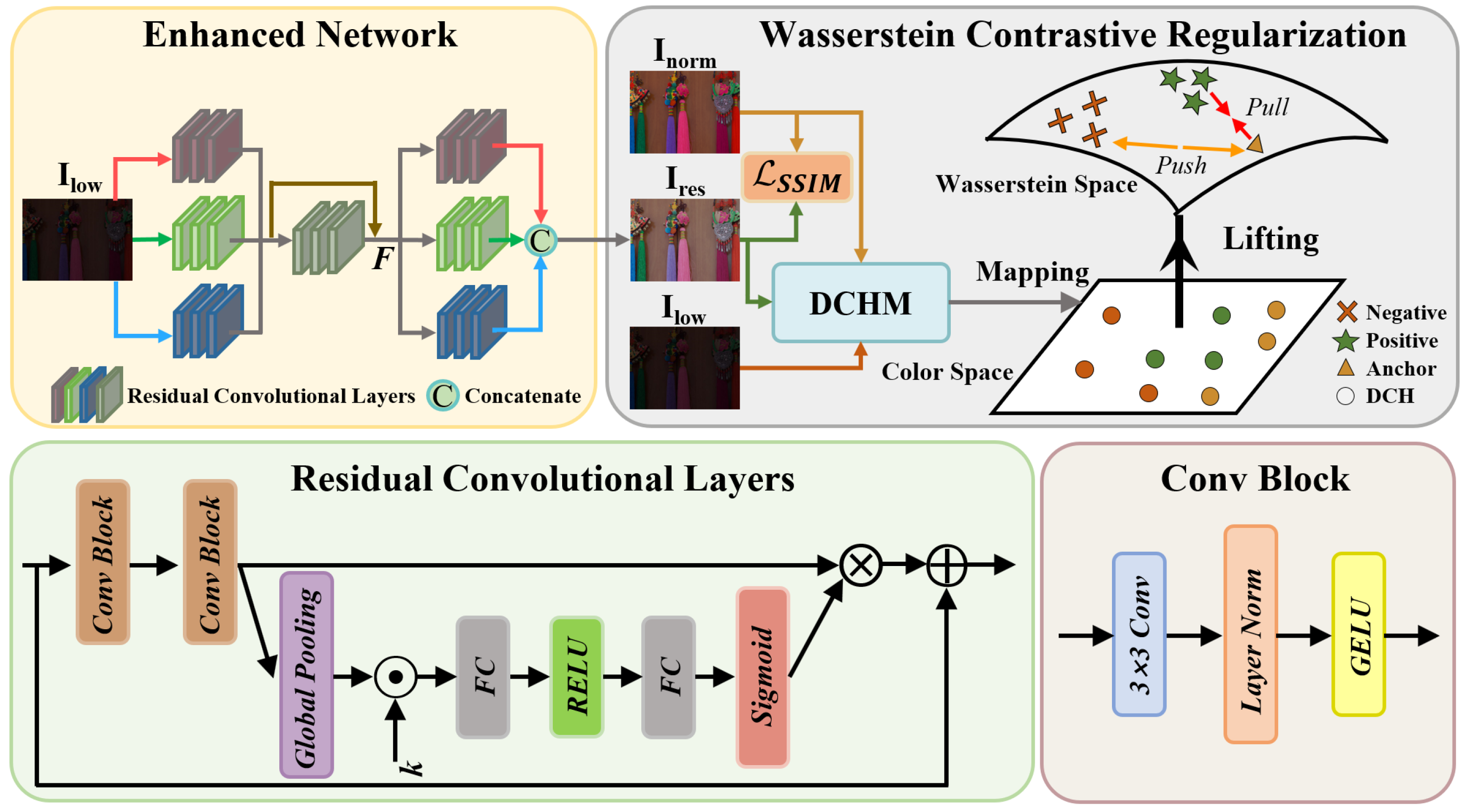
3.1. Overall Pipeline

Figure 2 illustrates the overall framework of our WCR. Given a low-light image ${\mathit{I}}_{\mathit{low}}\in {\mathbb{R}}^{H\times W\times 3}$, which has a height of H and a width of W, we first employ a lightweight network backbone composed of three parallel residual convolution layers followed by a residual layer to extract the low-level features $\mathit{F}\in {\mathbb{R}}^{H\times W\times C}$ with channel number C. Subsequently, $\mathit{F}$ passes through three sets of residual convolution layers to decouple and refine the prediction for each RGB channel, yielding ${\mathit{I}}_{\mathit{i}}\in {\mathbb{R}}^{H\times W\times 1}$ for channel $i=r,g,b$. Next, ${\mathit{I}}_{\mathit{r}},{\mathit{I}}_{\mathit{g}}$ and ${\mathit{I}}_{\mathit{b}}$ are merged along the channel axis to yield the restored image ${\mathit{I}}_{\mathit{res}}\in {\mathbb{R}}^{H\times W\times 3}$. Following this, the DCHM projects ${\mathit{I}}_{\mathit{low}}$, ${\mathit{I}}_{\mathit{res}}$, and the normal-light image ${\mathit{I}}_{\mathit{norm}}$ into the color space, resulting in the corresponding DCH representations ${\overrightarrow{\mathit{h}}}_{\mathit{low}}$, ${\overrightarrow{\mathit{h}}}_{\mathit{res}}$, and ${\overrightarrow{\mathit{h}}}_{\mathit{norm}}\in {\mathbb{R}}^{3d}$, where each CH representation $\overrightarrow{\mathit{h}}=[{\overrightarrow{\mathit{h}}}_{\mathit{r}},{\overrightarrow{\mathit{h}}}_{\mathit{g}},{\overrightarrow{\mathit{h}}}_{\mathit{b}}]$, which concatenates the d-dimensional CH ${\overrightarrow{\mathit{h}}}_{\mathit{i}}\in {\mathbb{R}}^d,i=r,g,b$ of each channel i. Then, we utilize the WD to measure the similarity between ${\overrightarrow{\mathit{h}}}_{\mathit{res}}$ and ${\overrightarrow{\mathit{h}}}_{\mathit{norm}}$, which constructs the WD loss that preserves the color consistency between the restored image and the normal-light image. Afterwards, ${\overrightarrow{\mathit{h}}}_{\mathit{res}}$, ${\overrightarrow{\mathit{h}}}_{\mathit{low}}$, and ${\overrightarrow{\mathit{h}}}_{\mathit{norm}}$ are taken as the anchor, negative, and positive sample representations, respectively, and we use the WD to measure the similarity among the positive/negative and the anchor samples, which constructs the CL loss that pulls the anchors closer to the positive samples while pushing the anchors farther away from the negative samples. The WD loss and the CL loss are then combined to construct the WCR loss. Finally, we jointly optimize the network by combining the structure similarity index measure (SSIM) loss [38] and the WCR loss.

In the subsequent sections, we will present the key designs including DCHM and WCR loss in detail.

3.2. DCHM

The computation of CH is nondifferential, which means it cannot be learned in an end-to-end manner. To address this issue, we designed the DCHM to use the kernel density estimation (KDE) [39] to approximate the CH.

Specifically, taking the channel of the red color as an example, we normalize the intensity of image pixel i to ${\mathit{I}}_{\mathit{r}}\left(i\right)\in [0,1]$. Then, the KDE estimates the density $D_r$ in the red color channel as follows:

$$D_r\left(x\right)=\frac{1}{SW}\sum _{i\in \mathsf{\Delta }}K\left(\frac{{\mathit{I}}_{\mathit{r}}\left(i\right)-x}{W}\right),$$

(1)

where $x\in [0,1]$, $S=\left|\mathsf{\Delta }\right|$ is the count of pixels in channel r, W is the bandwidth, and $K\left(x\right)=\sigma \left(x\right)(1-\sigma (x\left)\right)$ is the kernel function chose as the derivative of the Sigmoid function $\sigma \left(x\right)=1/(1+exp(-x\left)\right)$. Then, we divide interval $[0,1]$ into N subintervals, and each interval is denoted as $B_n=[\frac{n-1}{N},\frac{n}{N}]$, where $n\in [1,N]$. Furthermore, the likelihood of a pixel in channel r being assigned to the n-th bin in the histogram can be expressed as

$${\mathcal{P}}_r\left(n\right)={\int }_{I_n}{D}_r\left(x\right)dx=\frac{1}{S}\sum _{i\in \mathsf{\Delta }}\left[\sigma \left(\frac{{\mathit{I}}_{\mathit{r}}\left(i\right)-\frac{n-1}{N}}{W})-\sigma (\frac{{\mathit{I}}_{\mathit{r}}\left(i\right)-\frac{n}{N}}{W}\right)\right],$$

(2)

where $\sigma (·)$ is a Sigmoid function that approximates the unit step function. As illustrated by Figure 3, each pixel is represented as an N-dimensional smoothed one-hot vector and the function ${\mathcal{P}}_r\left(n\right)$ provides the value of the n-th bin in a DCH. In addition, to obtain the n-th bin of the histogram, we accumulate the values of all pixels in the n-th channel. Finally, the DH is defined as

$${\overrightarrow{\mathit{h}}}_{\mathit{r}}={\{{\mu }_n,{\mathcal{P}}_r\left(n\right)\}}_{n=1}^N,$$

(3)

where ${\mu }_n$ denotes the center of $B_n$.

The DCHs ${\overrightarrow{\mathit{h}}}_{\mathit{g}}$ and ${\overrightarrow{\mathit{h}}}_{\mathit{b}}$ can be calculated in the same way as ${\overrightarrow{\mathit{h}}}_{\mathit{r}}$ (3). Note that the DCHM can produce a smoothing histogram that can minimize undesired gradient effects. This is helpful to keep the color consistency, which is essential to LLIE.

3.3. WCR Loss

The WCR loss is defined as follows:

$${\mathcal{L}}_{WCR}={\mathcal{L}}_{WD}({\overrightarrow{\mathit{h}}}_{\mathit{res}},{\overrightarrow{\mathit{h}}}_{\mathit{norm}})+{\mathcal{L}}_{CL}({\overrightarrow{\mathit{h}}}_{\mathit{res}},{\overrightarrow{\mathit{h}}}_{\mathit{low}},{\overrightarrow{\mathit{h}}}_{\mathit{norm}}),$$

(4)

where the WD loss ${\mathcal{L}}_{WD}$ is to preserve the color consistency between the restored image and the reference image in normal lighting conditions, while the CL loss ${\mathcal{L}}_{CL}$ aims to minimize the residual noise in the restored image using guidance from the low-light image.

WD loss. The WD [40] computes the minimum average distance that needs to be covered when transporting data from two distributions. Given two probability distributions $\mathit{p}\sim \mathcal{P}$ and $\mathit{q}\sim \mathcal{Q}$, the WD between $\mathcal{P}$ and $\mathcal{Q}$ is defined as [40]

$$\mathcal{D}(\mathcal{P},\mathcal{Q})=\underset{\gamma \sim \mathsf{\Gamma }(\mathcal{P},\mathcal{Q})}{inf}{\int }_{\mathcal{M}\times \mathcal{M}}c(\mathit{p},\mathit{q})d\gamma (\mathit{p},\mathit{q}),$$

(5)

where $\mathsf{\Gamma }(\mathcal{P},\mathcal{Q})$ represents all possible couplings of $\mathcal{P}\left(\mathit{p}\right)$ and $\mathcal{Q}\left(\mathit{q}\right)$; $c(·)$ denotes a point-wise cost function that quantifies the dissimilarity between $\mathit{p}$ and $\mathit{q}$; $\mathcal{M}$ represents the space of $\mathit{p}$ and $\mathit{q}$; and $\gamma (\mathit{p},\mathit{q})$ represents a joint distribution that satisfies ${\int }_{\mathcal{M}}\gamma (\mathit{p},\mathit{q})d\mathit{q}=\mathcal{P}\left(\mathit{p}\right)$ and ${\int }_{\mathcal{M}}\gamma (\mathit{p},\mathit{q})d\mathit{p}=\mathcal{Q}\left(\mathit{q}\right)$.

The discrete WD of (5) can be formulated as [40]

$$\begin{array}{ccc}\hfill \mathcal{D}(\mathcal{P},\mathcal{Q})=\underset{\mathit{\pi }}{min}& & \sum _{i=1}^N\sum _{j=1}^N{\mathit{\pi }}_{ij}c({\mathit{p}}_i,{\mathit{q}}_j)=\underset{\mathit{\pi }}{min}〈\mathit{\pi },\mathit{C}〉,\hfill \\ \hfill s.t.& & \sum _{i=1}^N{\mathit{\pi }}_{ij}=d_j,\sum _{j=1}^N{\mathit{\pi }}_{ij}=s_i,\hfill \\ & & \sum _{i=1}^N{s}_i=\sum _{j=1}^N{d}_j,\hfill \\ & & {\mathit{\pi }}_{ij}\ge 0,i=1,2,\cdots ,N,j=1,2,\cdots ,N,\hfill \end{array}$$

(6)

where $\mathit{\pi }$ represents the discrete joint probability for $\mathit{p}$ and $\mathit{q}$, which can be thought of as the transportation plan. The cost matrix, denoted as $\mathit{C}$, is defined by ${\mathit{C}}_{ij}=c({\mathit{p}}_i,{\mathit{q}}_j)={\mathit{p}}_i^{\top }{\mathit{q}}_j$, where ${\mathit{p}}_i$ and ${\mathit{q}}_j$ are elements of $\mathit{p}$ and $\mathit{q}$, respectively. The inner product $〈\mathit{\pi },\mathit{C}〉=Tr\left({\mathit{\pi }}^{\mathrm{T}}\mathit{C}\right)$ is computed using the trace operator $Tr\left(\right)$, and $s_i$ denotes the inventory or quantity of goods available with the i-th supplier, while $d_j$ represents the demand or quantity of goods required by the j-th consumer in the context of optimal transportation theory [40]. To find the global optimum for (6), linear programming is typically used. However, due to its nondifferentiability, this approach is not compatible with current deep learning frameworks. To address this issue, we employ the Sinkhorn distance [41], which introduces a convex regularization term into (6). This regularization term can be expressed as

$$\mathcal{D}(\mathcal{P},\mathcal{Q})=\underset{\mathit{\pi }}{min}\sum _{i=1}^N\sum _{j=1}^N{\mathit{\pi }}_{ij}c({\mathit{p}}_i,{\mathit{q}}_j)+\alpha \mathcal{H}\left(\mathit{\pi }\right),$$

(7)

where $\mathcal{H}\left(\mathit{\pi }\right)={\sum }_{i,j}{\mathit{\pi }}_{ij}log{\mathit{\pi }}_{ij}$, and $\alpha$ is a hyperparameter that controls the relative importance of the entropy loss on $\mathit{\pi }$. The Sinkhorn distance is a differential module that can be readily embedded into the network for end-to-end training.

We measure the WD between ${\overrightarrow{\mathit{h}}}_{\mathit{res}}$ and ${\overrightarrow{\mathit{h}}}_{\mathit{norm}}$ via optimizing the problem (7) to learn CH representation between the restored image and the normal-light image, yielding the WD loss as

$${\mathcal{L}}_{WD}=\mathcal{D}({\overrightarrow{\mathit{h}}}_{\mathit{res}},{\overrightarrow{\mathit{h}}}_{\mathit{norm}}).$$

(8)

By capturing the global color statistics of the normal-light image, ${\mathcal{L}}_{WD}$ can enhance the realism and richness of color in the restored image, while maintaining color consistency, as shown in Figure 4.

CL loss. When optimizing a network only using normal-light images, negative representations present in the low-light images are neglected. This leads to the restored image undergoing severe residual noise. To address this issue, inspired by CL [21,22], we propose a CL loss that is a triplet loss [42], which takes the normal-light images as positive samples, the low-light images as negative samples, and the restored images as anchor samples. As shown in Figure 5, the CL loss aims to learn a DCH representation of the restored image that is closer to the normal-light image than the low-light image, which can formulated as

$$\mathcal{D}({\overrightarrow{\mathit{h}}}_{\mathit{res}},{\overrightarrow{\mathit{h}}}_{\mathit{norm}})+\rho <\mathcal{D}({\overrightarrow{\mathit{h}}}_{\mathit{res}},{\overrightarrow{\mathit{h}}}_{\mathit{low}}),$$

(9)

where $\rho$ represents the margin, which ensures that the features of the samples do not collapse into a very small Wasserstein space subjected to the metric $\mathcal{D}$ (5).

Then, we define $({\overrightarrow{\mathit{h}}}_{\mathit{res}}^i,{\overrightarrow{\mathit{h}}}_{\mathit{norm}}^j)$ as the positive sample pairs and $({\overrightarrow{\mathit{h}}}_{\mathit{res}}^i,{\overrightarrow{\mathit{h}}}_{\mathit{low}}^j)$ as negative sample pairs, where i and j denote the sample number within a batch. It should be noted that i may or may not be equal to j. That is, to ensure the generalization of the network, the normal-light and low-light images can be unpaired with the restored images. Following this, according to (9), the CL loss can be written as

$${\mathcal{L}}_{CL}=\sum _i^{bs}\sum _j^{bs}{[\mathcal{D}({\overrightarrow{\mathit{h}}}_{\mathit{res}}^i,{\overrightarrow{\mathit{h}}}_{\mathit{norm}}^j)-\mathcal{D}({\overrightarrow{\mathit{h}}}_{\mathit{res}}^i,{\overrightarrow{\mathit{h}}}_{\mathit{low}}^j)+\rho ]}_{+},$$

(10)

where $bs$ denotes the batch size.

3.4. Total Loss

Apart from the proposed WCR loss, we incorporate the SSIM loss [38] as an additional constraint to enhance the restoration of structural details, which is defined as

$${\mathcal{L}}_{SSIM}=1-SSIM({\mathit{I}}_{\mathit{res}},{\mathit{I}}_{\mathit{norm}}),$$

(11)

where the structural similarity function denoted as $SSIM(·)$, which is described in [38], is expressed as follows:

$$SSIM({\mathit{I}}_1,{\mathit{I}}_2)=\frac{2{\mu }_1{\mu }_2+c_1}{{\mu }_1^2+{\mu }_2^2+c_1}·\frac{2{\sigma }_1+c_2}{{\sigma }_1^2+{\sigma }_2^2+c_1},$$

(12)

Finally, the total loss of our proposed WCR is defined as

$${\mathcal{L}}_{total}={\lambda }_1{\mathcal{L}}_{SSIM}+{\lambda }_2{\mathcal{L}}_{WCR},$$

(13)

where ${\lambda }_1$ and ${\lambda }_2$ are two trade-off parameters. Among the total loss ${\mathcal{L}}_{total}$, ${\mathcal{L}}_{SSIM}$ (11) is utilized to reconstruct the image in structure level and ${\mathcal{L}}_{WCR}$ (4) is used as a regularization term to learn the DCH representations to keep color consistency and remove the residual noise; where ${\mathit{I}}_1,{\mathit{I}}_2\in {\mathbb{R}}^{H\times W\times 3}$ are two images, ${\mu }_1,{\mu }_2\in \mathbb{R}$ are their mean values, ${\sigma }_1,{\sigma }_2\in \mathbb{R}$ are their variances, and $c_1$ and $c_2$ are constant parameters to avoid division by zero.

4. Experiments

4.1. Implementation Details

The WCR method was designed to be trainable end-to-end, eliminating the need for progressive training or extensive pretraining. All experiments were conducted using the Python environment and the PyTorch framework, with an NVIDIA GeForce RTX 3090. The network was trained on $100\times 100$ randomly cropped patches, and the original image size was used for testing. No data augmentation method was employed in our approach. The AdamW optimizer [43] was utilized with a batch size of 16 and an initial learning rate of $8\times {10}^{-4}$, which were steadily decreased to $8\times {10}^{-8}$. For the trade-off parameters ${\lambda }_1$ and ${\lambda }_2$ in ${\mathcal{L}}_{total}$ (13), we set them to 1 and 0.1, respectively. For the LOL dataset [13], we trained the model for 100 epochs and the number of patches per image was 30. For the MIT-Adobe FiveK dataset [23], we trained the model for 20 epochs and the number of patches per image was 38. For the UIEB dataset [24], we trained the model for 100 epochs and the number of patches per image was 35.

4.2. Evaluation Datasets and Metrics

Evaluation datasets. For the LLIE task, we used the LOL real dataset [13]. LOL contains 500 pairs of extremely dark images of $400\times 600$ resolution. It was divided into 485 training image pairs and 15 image pairs for testing. In order to comprehensively assess the efficacy of the proposed WCR method, we also conducted experiments on the widely used image retouching dataset MIT-Adobe FiveK [23] and the underwater image enhancement dataset UIEB [24]. The MIT-Adobe FiveK dataset comprises 5000 images with diverse lighting intensities and varying resolutions. We followed the method [44] that splits the dataset by using the first 4500 images for training and the remaining 500 images for testing. The UIEB dataset is a commonly used benchmark for underwater image enhancement, which mainly focuses on color adjustment and noise removal. The UIEB dataset consists of a total of 950 underwater images captured in real-world scenarios, with 890 of them having corresponding reference images. The division of the UIEB dataset into training and testing sets aligns with the partitioning utilized in PUIE [45].

Evaluation metrics. For the LOL dataset, we report the PSNR, the SSIM, and the learned perceptual image patch similarity LPIPS [46] scores for quantitative evaluation. We also report the WD score, which measures the Wasserstein distance between the histogram of the restored image and the histogram of its corresponding normal-light image. To ensure fairness and consistency in evaluation, we utilized pretrained models provided by other comparative methods and assessed the performance under the same test metric settings, considering that different platforms can lead to varying test results. Additionally, we measured the model parameter size and computational complexity using Params and FLOPs. For the MIT-Adobe FiveK dataset and the UIEB dataset, we conducted the analysis using PSNR and SSIM metrics. To conduct a more comprehensive accuracy comparison between the two sets of predictions, we employed the two-sample Kolmogorov–Smirnov (K-S) test [47]. This statistical test examines whether the color histogram distributions of the output and the reference exhibit consistency.

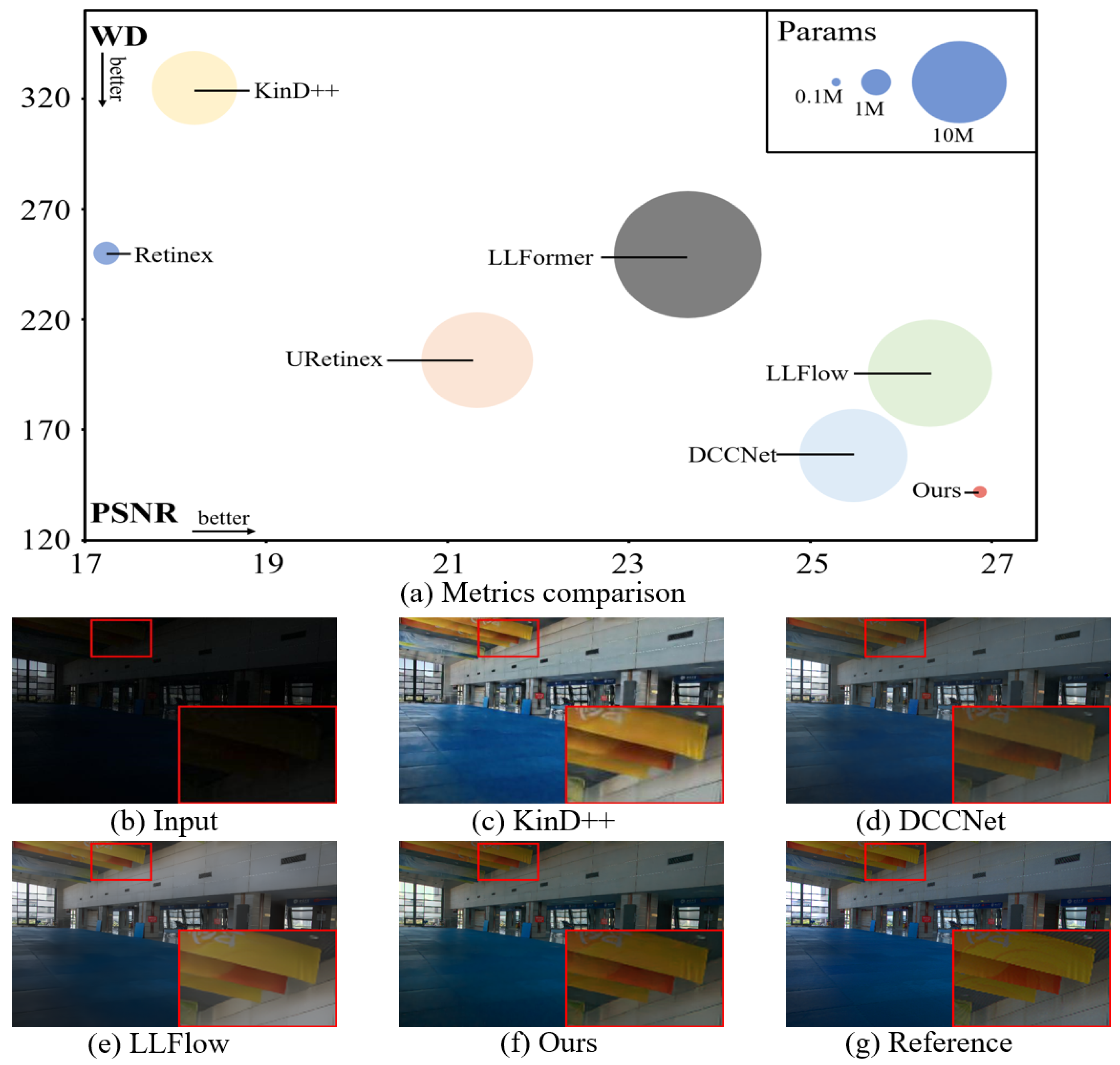
4.3. Quantitative Enhancement Results

The quantitative comparison results of our novel WCR method against state-of-the-art LLIE methods on the LOL dataset are presented in

Table 1. Quantitative comparison on the LOL dataset [13] based on various metrics such as PSNR, SSIM, LPIPS, WD, Params, and FLOPs. A higher value is preferred for metrics denoted by ↑ (e.g., PSNR and SSIM), while a smaller value is preferred for metrics denoted by ↓ (e.g., WD, LPIPS, Params, and FLOPs). Red text denotes the best result, while blue text indicates the second best.

Method	PSNR↑	SSIM↑	LPIPS↓	WD↓	Params (M)↓	FLOPs (G)↓
Retinex(BMVC’18) [13]	18.04	0.67	0.389	250.07	0.84	587.47
KinD(ACMMM’19) [27]	18.15	0.82	0.131	261.55	8.16	356.72
KinD++(IJCV’21) [5]	18.21	0.83	0.148	264.91	8.28	2532
MIRNet(ECCV’20) [48]	23.91	0.88	0.093	152.42	31.79	2882.24
URetinex(CVPR’22) [14]	21.33	0.88	0.096	201.64	15.10	-
MAXIM(CVPR’22) [44]	25.73	0.89	0.075	158.42	14.14	216
LLFormer(AAAI’23) [26]	23.65	0.87	0.107	160.37	24.52	-
DCC(CVPR’22) [7]	25.48	0.89	0.091	148.25	13.19	270.47
LLFLow(AAAI’22) [6]	26.32	0.91	0.092	195.62	17.42	1050
Ours	26.87	0.90	0.083	141.80	0.24	55.3

. The results demonstrate outstanding performance in comparison to other state-of-the-art methods, ranking within the top two for all metrics. In particular, our proposed method achieved the best PSNR = 26.87 dB and WD = 141.8. The PSNR metric focuses on evaluating the quality of image denoising, while the WD metric emphasizes color consistency in image restoration. It is worth noting that, unlike previous methods that have to strike a balance between these two metrics, our WCR method can achieve both excellent denoising performance and color consistency. In addition, the proposed WCR method was only utilized for training without increasing the model’s parameter count and computational requirements. Therefore, the WCR method also achieved optimal performance in terms of Params = 0.24 M and FLOPs = 55.3 G.

Table 2. Quantitative comparison on the MIT-Adobe FiveK dataset [23] and the UIEB dataset [24] in terms of PSNR and SSIM. ↑(↓) denotes that larger(smaller) values lead to better quality. The red denotes the best performance and the blue denotes the second best.

Methods	FiveK		Methods	UIEB
	PSNR↑	SSIM↑		PSNR↑	SSIM↑
MBLLEN(BMVC’18) [25]	19.78	0.83	ReUIE(ICIP’14) [49]	17.53	0.77
KinD(ACMMM’19) [27]	14.54	0.74	IBLA(TIP’17) [50]	18.51	0.76
DSLR(TMM’20) [51]	16.63	0.78	WaterNet(TIP’19) [24]	19.81	0.86
DPE(CVPR’18) [52]	24.08	0.92	Haze-line(TPAMI’20) [53]	14.97	0.67
IRN(ICCV’21) [54]	24.27	0.90	LC-Net(TMM’21) [55]	18.54	0.84
CLUT(ACMMM’22) [56]	25.55	0.93	Ucolor(TIP’21) [57]	21.65	0.84
MAXIM(CVPR’22) [44]	26.15	0.95	PUIE(ECCV’22) [45]	21.86	0.87
Ours	26.66	0.96	Ours	22.32	0.90

lists the qualitative results compared to the state-of-the-art methods for the tasks of image retouching and underwater image enhancement on the MIT-Adobe FiveK dataset and the UIEB dataset, respectively. As indicated in Table 2, our proposed WCR method outperformed the existing LLIE methods and established new state-of-the-art results across all evaluation metrics. Our method achieves a PSNR = 26.66 dB and SSIM = 0.96 on the MIT-Adobe FiveK dataset, with a gain of 0.51 dB and $1\%$ over the competing counterpart MAXIM [44]. Moreover, for the UIEB dataset, our WCR method achieved a PSNR = 22.32 dB and SSIM = 0.91, with a gain of 0.46 dB and $3\%$ over the competing counterpart PUIE [45].

Table 3. Comparison of results from the two-sample K-S test on the LOL test set. S denotes the test statistic, C represents the critical value, and RGB represents the red, green, and blue channels, respectively. Critical values displayed in blue font indicate that they are smaller than the test statistic, leading to the rejection of the null hypothesis. Critical values displayed in red font indicate that they are greater than the test statistic, hence the null hypothesis cannot be rejected.

Method	S (R)	C (R)	S (G)	C (G)	S (B)	C (B)
LLFlow	0.1250	0.0365	0.0781	0.4160	0.1289	0.0283
DCCNet	0.1133	0.0748	0.0625	0.7004	0.1523	0.0052
Our	0.0781	0.4160	0.0703	0.5524	0.0977	0.1741

presents the consistency outcomes achieved through the two-sample K-S test conducted on the LOL test set. The test assumes that the distribution of the output aligns with that of the reference graph. It is important to note that the results displayed are the average values across all test images. As shown in Table 3, our proposed method demonstrated critical values in the RGB three channels that surpassed the test statistics, leading us to fail to reject the null hypothesis. Conversely, both LLFlow and DCCNet, the current state-of-the-art methods, exhibited inconsistent distribution in their color channels. This substantiates our method’s capability to recover a more precise color representation.

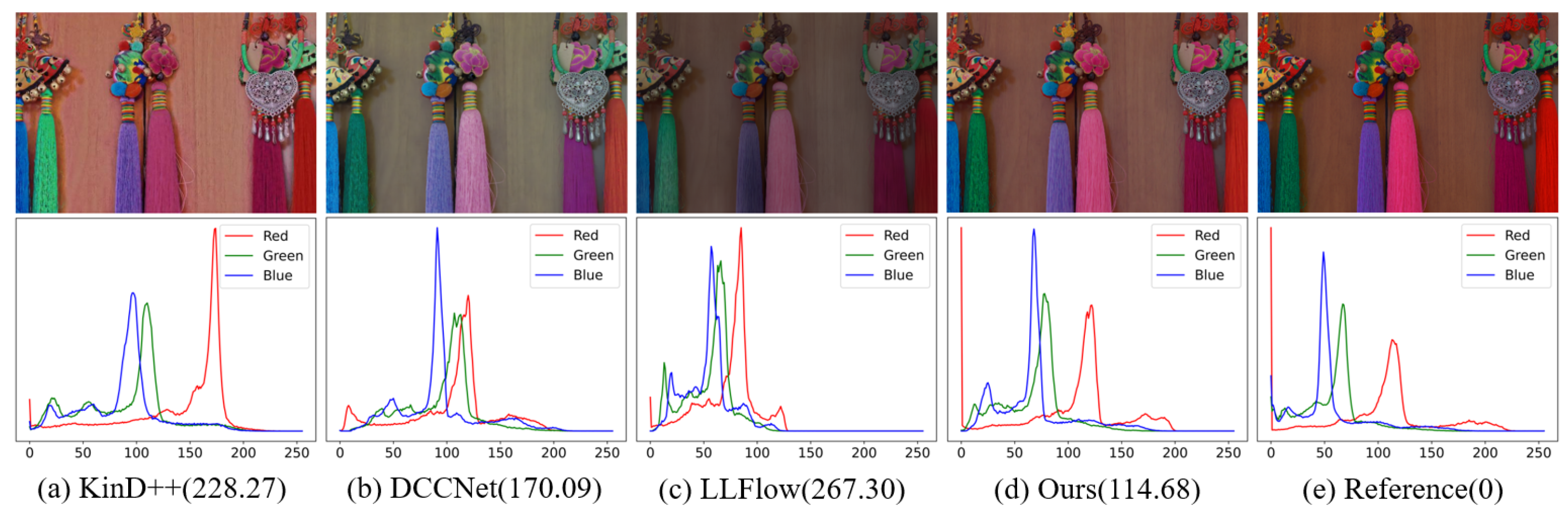
4.4. Visual Image Analysis and Evaluations

In terms of visual performance, we further compared our method with state-of-the-art approaches on the LOL dataset, the results of which are presented in Figure 6 and Figure 7. As shown in Figure 6, KinD++ enhanced the image with an inferior visual quality. DCCNet achieved a suboptimal WD, but it did not model the noise distribution hidden in low-light images, resulting in a lower PSNR. In contrast, LLFlow takes low-light images as a condition and applies normalization flow for denoising, but it neglects to capture global color statistics differences between the restored images and the normal-light images, leading to color deviation with a larger WD. Our model achieved visual higher quality with crisper details, more real colors, and less noise. In Figure 7, a selection of images from the LOL dataset is showcased, accompanied by the enhancement outcomes achieved through various techniques, including the enlarged details. While KinD++ was effective in improving brightness, it introduced distorted colors and noise. LLFlow performed well in noise reduction, but excessive smoothing led to unrealistic results with overexposure in local regions. Our proposed model clearly outperformed it, demonstrating the superiority of our proposed WCR method. Figure 8 shows some qualitative results from the FiveK dataset and the UIEB dataset. It is evident that the WCR method attained excellent restoration of visual effects in the image retouching and underwater image enhancement, including more realistic color and reduced noise.

4.5. Ablation Study

Ablation experiments were conducted to evaluate the efficacy of our proposed ${\mathcal{L}}_{WD}$ and ${\mathcal{L}}_{CL}$ in comparison to the commonly used ${\mathcal{L}}_1$ and ${\mathcal{L}}_{SSIM}$. Moreover, we performed additional ablation experiments on our proposed WCR using the convolution-based Unet [58] and the latest transformer-based LLFormer [26] model. The results are reported in

Table 4. Ablation study on the LOL dataset [13] for different loss. Bold represents the best result.

Module Variants				PSNR↑	SSIM↑	LPIPS↓	WD↓
${\mathcal{L}}_{\mathit{1}}$	${\mathcal{L}}_{\mathit{SSIM}}$	${\mathcal{L}}_{\mathit{WD}}$	${\mathcal{L}}_{\mathit{CL}}$
✓				22.73	0.83	0.157	207.34
✓		✓		24.37	0.86	0.104	151.17
✓		✓	✓	25.98	0.87	0.083	144.12
	✓			23.34	0.85	0.138	199.96
	✓	✓		25.46	0.88	0.090	146.76
	✓	✓	✓	26.87	0.90	0.083	141.80

and

Table 5. Ablation study results of different models with convolutional neural network architecture and transformer architecture on the LOL dataset [13]. Bold indicates the amount of change in the corresponding metrics.

Model	PSNR↑	SSIM↑	LPIPS↓	WD↓
Unet [58] w/o WCR	17.74	0.83	0.164	254.36
Unet w WCR	19.52 (+1.78)	0.85	0.137	200.94 (−53.42)
LLFormer [26] w/o WCR	23.65	0.87	0.107	160.37
LLFormer w WCR	25.17 (+1.52)	0.88	0.094	133.58 (−26.79)

, which clearly show that all the key designs contribute to the best performance of the full model.

Without ${\mathcal{L}}_{WD}$, our method achieved a PSNR = 22.73 dB, SSIM = 0.83, LPIPS = 0.157, and WD = 207.34, which are lower than the proposed model with ${\mathcal{L}}_{WD}$ by $1.64$ dB, $3\%$, $0.053$, and $56.17$, respectively. We then further plugged ${\mathcal{L}}_{CL}$, achieving a gain of 1.61 dB, $1\%$, $0.021$, and $7.05$ in terms of PSNR, SSIM, LPIPS, and WD, respectively, as compared to the complementary technique. The ablation experiment using ${\mathcal{L}}_{SSIM}$ as the baseline showed similar performance changes, but using ${\mathcal{L}}_{SSIM}$ and our proposed WCR method resulted in a higher PSNR = 26.87 dB, SSIM = $0.90$, LPIPS = $0.083$, and WD = $141.80$ than using ${\mathcal{L}}_1$ and the proposed WCR method.

In order to assess the efficacy and applicability of the WCR method, we replaced the network with two different architectures: Unet [58] and LLFormer [26], while keeping the training settings consistent with our previous experiments. Table 4 shows that without the WCR method, both models achieved a lower performance, particularly in terms of PSNR and WD. The higher PSNR and lower WD values obtained with our proposed WCR method demonstrate its ability to maintain color consistency while removing noise. Figure 9 shows that the color distribution statistics of the restored images obtained using our proposed WCR method are more similar to those of normal-light images, particularly for challenging samples located off-center. Moreover, Figure 10 shows that the model trained without the WCR method produced more obvious color deviation and noise. The superiority of our proposed WCR method in modeling the image representations was confirmed by both the quantitative and qualitative results.

5. Discussion

We provide an efficient and effective WCR method to perform LLIE. The proposed WCR method efficiently models color distributions for effective noise removal and color consistency preservation. In comparison to existing SOTA methods, our model achieves more realistic image restoration with a lower parameter count and computational overheads, as demonstrated in Table 1 and Figure 6. Furthermore, the WCR method exhibits strong generalization, delivering optimal performance on image enhancement tasks using both the MIT FiveK dataset and the UIEB dataset, as shown in Table 2. This is attributed to our DCHM, which serves as a plug-and-play module, without adding to the model size or inference cost. Additionally, our proposed WCR method regularizes the CH representation of the restored images in Wasserstein space, ensuring color consistency while eliminating residual noise.

6. Conclusions

In this paper, we address the issue of keeping color consistency while removing noise in LLIE. To solve this problem, we propose a novel WCR method for LLIE, which regularizes the CH representation of the restored image. Specifically, we designed the DCHM to learn the image CH representation in an end-to-end manner in Wasserstein space. Then, the WCR loss takes the normal-light images as positive samples, the low-light images as negative samples, and the restored images as anchor samples for contrastive learning to recover the real color representation and reduces the residual noise. The favorable performance of our proposed WCR method was showcased in our experiments conducted on the LOL dataset, MIT-Adobe FiveK dataset, and UIEB dataset, outperforming several state-of-the-art methods.

References

1. Sultani, W.; Chen, C.; Shah, M. Real-world anomaly detection in surveillance videos. In Proceedings of the IEEE Conference on Computer Vision and Pattern Recognition, Salt Lake City, UT, USA, 18–23 June 2018; pp. 6479–6488. [Google Scholar]
2. Lamba, M.; Rachavarapu, K.K.; Mitra, K. Harnessing multi-view perspective of light fields for low-light imaging. IEEE Trans. Image Process. 2020, 30, 1501–1513. [Google Scholar] [CrossRef] [PubMed]
3. Wang, W.; Yang, W.; Liu, J. Hla-face: Joint high-low adaptation for low light face detection. In Proceedings of the IEEE/CVF Conference on Computer Vision and Pattern Recognition, Nashville, TN, USA, 20–25 June 2021; pp. 16195–16204. [Google Scholar]
4. Liang, J.; Wang, J.; Quan, Y.; Chen, T.; Liu, J.; Ling, H.; Xu, Y. Recurrent exposure generation for low-light face detection. IEEE Trans. Multimed. 2021, 24, 1609–1621. [Google Scholar] [CrossRef]
5. Zhang, Y.; Guo, X.; Ma, J.; Liu, W.; Zhang, J. Beyond brightening low-light images. Int. J. Comput. Vis. 2021, 129, 1013–1037. [Google Scholar] [CrossRef]
6. Wang, Y.; Wan, R.; Yang, W.; Li, H.; Chau, L.P.; Kot, A. Low-light image enhancement with normalizing flow. In Proceedings of the AAAI Conference on Artificial Intelligence, Pomona, CA, USA, 24–28 October 2022; Volume 36, pp. 2604–2612. [Google Scholar]
7. Zhang, Z.; Zheng, H.; Hong, R.; Xu, M.; Yan, S.; Wang, M. Deep Color Consistent Network for Low-Light Image Enhancement. In Proceedings of the IEEE/CVF Conference on Computer Vision and Pattern Recognition, New Orleans, LA, USA, 18–24 June 2022; pp. 1899–1908. [Google Scholar]
8. Kim, B.; Lee, S.; Kim, N.; Jang, D.; Kim, D.S. Learning color representations for low-light image enhancement. In Proceedings of the IEEE/CVF Winter Conference on Applications of Computer Vision, Waikoloa, HI, USA, 3–8 January 2022; pp. 1455–1463. [Google Scholar]
9. Wu, Y.; Pan, C.; Wang, G.; Yang, Y.; Wei, J.; Li, C.; Shen, H.T. Learning Semantic-Aware Knowledge Guidance for Low-Light Image Enhancement. In Proceedings of the IEEE/CVF Conference on Computer Vision and Pattern Recognition, Vancouver, BC, Canada, 18–22 June 2023; pp. 1662–1671. [Google Scholar]
10. Yeganeh, H.; Ziaei, A.; Rezaie, A. A novel approach for contrast enhancement based on histogram equalization. In Proceedings of the 2008 International Conference on Computer and Communication Engineering, Kuala Lumpur, Malaysia, 13–15 May 2008; pp. 256–260. [Google Scholar]
11. Wang, S.; Zheng, J.; Hu, H.M.; Li, B. Naturalness preserved enhancement algorithm for non-uniform illumination images. IEEE Trans. Image Process. 2013, 22, 3538–3548. [Google Scholar] [CrossRef] [PubMed]
12. Ren, X.; Yang, W.; Cheng, W.H.; Liu, J. LR3M: Robust low-light enhancement via low-rank regularized retinex model. IEEE Trans. Image Process. 2020, 29, 5862–5876. [Google Scholar] [CrossRef] [PubMed]
13. Wei, C.; Wang, W.; Yang, W.; Liu, J. Deep retinex decomposition for low-light enhancement. arXiv 2018, arXiv:1808.04560. [Google Scholar]
14. Wu, W.; Weng, J.; Zhang, P.; Wang, X.; Yang, W.; Jiang, J. URetinex-Net: Retinex-Based Deep Unfolding Network for Low-Light Image Enhancement. In Proceedings of the IEEE/CVF Conference on Computer Vision and Pattern Recognition, New Orleans, LA, USA, 18–24 June 2022; pp. 5901–5910. [Google Scholar]
15. Li, C.; Guo, J.; Porikli, F.; Pang, Y. LightenNet: A convolutional neural network for weakly illuminated image enhancement. Pattern Recognit. Lett. 2018, 104, 15–22. [Google Scholar] [CrossRef]
16. Zhang, F.; Li, Y.; You, S.; Fu, Y. Learning temporal consistency for low light video enhancement from single images. In Proceedings of the IEEE/CVF Conference on Computer Vision and Pattern Recognition, Nashville, TN, USA, 20–25 June 2021; pp. 4967–4976. [Google Scholar]
17. Jiang, H.; Zheng, Y. Learning to see moving objects in the dark. In Proceedings of the IEEE/CVF International Conference on Computer Vision, Seoul, Republic of Korea, 27 October–2 November 2019; pp. 7324–7333. [Google Scholar]
18. Wang, Y.; Cao, Y.; Zha, Z.J.; Zhang, J.; Xiong, Z.; Zhang, W.; Wu, F. Progressive retinex: Mutually reinforced illumination-noise perception network for low-light image enhancement. In Proceedings of the 27th ACM International Conference on Multimedia, Nice, France, 21–25 October 2019; pp. 2015–2023. [Google Scholar]
19. Lore, K.G.; Akintayo, A.; Sarkar, S. LLNet: A deep autoencoder approach to natural low-light image enhancement. Pattern Recognit. 2017, 61, 650–662. [Google Scholar] [CrossRef]
20. Dobrushin, R.L. Prescribing a system of random variables by conditional distributions. Theory Probab. Its Appl. 1970, 15, 458–486. [Google Scholar] [CrossRef]
21. Chen, T.; Kornblith, S.; Norouzi, M.; Hinton, G. A simple framework for contrastive learning of visual representations. In Proceedings of the International Conference on Machine Learning, PMLR, Virtual, 13–18 July 2020; pp. 1597–1607. [Google Scholar]
22. He, K.; Fan, H.; Wu, Y.; Xie, S.; Girshick, R. Momentum contrast for unsupervised visual representation learning. In Proceedings of the IEEE/CVF Conference on Computer Vision and Pattern Recognition, Seattle, WA, USA, 13–19 June 2020; pp. 9729–9738. [Google Scholar]
23. Bychkovsky, V.; Paris, S.; Chan, E.; Durand, F. Learning Photographic Global Tonal Adjustment with a Database of Input/Output Image Pairs. In Proceedings of the The Twenty-Fourth IEEE Conference on Computer Vision and Pattern Recognition, Colorado Springs, CO, USA, 20–25 June 2011. [Google Scholar]
24. Li, C.; Guo, C.; Ren, W.; Cong, R.; Hou, J.; Kwong, S.; Tao, D. An underwater image enhancement benchmark dataset and beyond. IEEE Trans. Image Process. 2019, 29, 4376–4389. [Google Scholar] [CrossRef]
25. Lv, F.; Lu, F.; Wu, J.; Lim, C. MBLLEN: Low-Light Image/Video Enhancement Using CNNs. In Proceedings of the BMVC, Newcastle, UK, 3–6 September 2018; Volume 220, p. 4. [Google Scholar]
26. Wang, T.; Zhang, K.; Shen, T.; Luo, W.; Stenger, B.; Lu, T. Ultra-High-Definition Low-Light Image Enhancement: A Benchmark and Transformer-Based Method. arXiv 2022, arXiv:2212.11548. [Google Scholar]
27. Zhang, Y.; Zhang, J.; Guo, X. Kindling the darkness: A practical low-light image enhancer. In Proceedings of the 27th ACM International Conference on Multimedia, Nice, France, 21–25 October 2019; pp. 1632–1640. [Google Scholar]
28. Guo, C.; Li, C.; Guo, J.; Loy, C.C.; Hou, J.; Kwong, S.; Cong, R. Zero-reference deep curve estimation for low-light image enhancement. In Proceedings of the IEEE/CVF Conference on Computer Vision and Pattern Recognition, Seattle, WA, USA, 13–19 June 2020; pp. 1780–1789. [Google Scholar]
29. Li, C.; Guo, C.; Loy, C.C. Learning to enhance low-light image via zero-reference deep curve estimation. IEEE Trans. Pattern Anal. Mach. Intell. 2021, 44, 4225–4238. [Google Scholar]
30. Ma, L.; Ma, T.; Liu, R.; Fan, X.; Luo, Z. Toward fast, flexible, and robust low-light image enhancement. In Proceedings of the IEEE/CVF Conference on Computer Vision and Pattern Recognition, New Orleans, LA, USA, 18–24 June 2022; pp. 5637–5646. [Google Scholar]
31. Xie, E.; Ding, J.; Wang, W.; Zhan, X.; Xu, H.; Sun, P.; Li, Z.; Luo, P. Detco: Unsupervised contrastive learning for object detection. In Proceedings of the IEEE/CVF International Conference on Computer Vision, Montreal, BC, Canada, 11–17 October 2021; pp. 8392–8401. [Google Scholar]
32. Wei, F.; Gao, Y.; Wu, Z.; Hu, H.; Lin, S. Aligning pretraining for detection via object-level contrastive learning. Adv. Neural Inf. Process. Syst. 2021, 34, 22682–22694. [Google Scholar]
33. Hu, H.; Cui, J.; Wang, L. Region-aware contrastive learning for semantic segmentation. In Proceedings of the IEEE/CVF International Conference on Computer Vision, Montreal, BC, Canada, 11–17 October 2021; pp. 16291–16301. [Google Scholar]
34. Wu, H.; Qu, Y.; Lin, S.; Zhou, J.; Qiao, R.; Zhang, Z.; Xie, Y.; Ma, L. Contrastive learning for compact single image dehazing. In Proceedings of the IEEE/CVF Conference on Computer Vision and Pattern Recognition, Nashville, TN, USA, 20–25 June 2021; pp. 10551–10560. [Google Scholar]
35. Huang, S.; Wang, K.; Liu, H.; Chen, J.; Li, Y. Contrastive semi-supervised learning for underwater image restoration via reliable bank. In Proceedings of the IEEE/CVF Conference on Computer Vision and Pattern Recognition, Vancouver, BC, Canada, 18–22 June 2023; pp. 18145–18155. [Google Scholar]
36. Liang, D.; Li, L.; Wei, M.; Yang, S.; Zhang, L.; Yang, W.; Du, Y.; Zhou, H. Semantically contrastive learning for low-light image enhancement. In Proceedings of the AAAI Conference on Artificial Intelligence, Pomona, CA, USA, 24–28 October 2022; Volume 36, pp. 1555–1563. [Google Scholar]
37. Fu, H.; Zheng, W.; Meng, X.; Wang, X.; Wang, C.; Ma, H. You Do Not Need Additional Priors or Regularizers in Retinex-Based Low-Light Image Enhancement. In Proceedings of the IEEE/CVF Conference on Computer Vision and Pattern Recognition, Vancouver, BC, Canada, 18–22 June 2023; pp. 18125–18134. [Google Scholar]
38. Wang, Z.; Bovik, A.C.; Sheikh, H.R.; Simoncelli, E.P. Image quality assessment: From error visibility to structural similarity. IEEE Trans. Image Process. 2004, 13, 600–612. [Google Scholar] [CrossRef]
39. Avi-Aharon, M.; Arbelle, A.; Raviv, T.R. Differentiable Histogram Loss Functions for Intensity-based Image-to-Image Translation. IEEE Trans. Pattern Anal. Mach. Intell. 2023, 45, 11642–11653. [Google Scholar] [CrossRef]
40. Villani, C. Optimal Transport: Old and New; Springer: Berlin/Heidelberg, Germany, 2009; Volume 338. [Google Scholar]
41. Cuturi, M. Sinkhorn distances: Lightspeed computation of optimal transport. Adv. Neural Inf. Process. Syst. 2013, 26, 2292–2300. [Google Scholar]
42. Schroff, F.; Kalenichenko, D.; Philbin, J. Facenet: A unified embedding for face recognition and clustering. In Proceedings of the IEEE Conference on Computer Vision and Pattern Recognition, Boston, MA, USA, 7–12 June 2015; pp. 815–823. [Google Scholar]
43. Loshchilov, I.; Hutter, F. Decoupled weight decay regularization. arXiv 2017, arXiv:1711.05101. [Google Scholar]
44. Tu, Z.; Talebi, H.; Zhang, H.; Yang, F.; Milanfar, P.; Bovik, A.; Li, Y. Maxim: Multi-axis mlp for image processing. In Proceedings of the IEEE/CVF Conference on Computer Vision and Pattern Recognition, New Orleans, LA, USA, 18–24 June 2022; pp. 5769–5780. [Google Scholar]
45. Fu, Z.; Wang, W.; Huang, Y.; Ding, X.; Ma, K.K. Uncertainty Inspired Underwater Image Enhancement. In Proceedings of the Computer Vision–ECCV 2022: 17th European Conference, Tel Aviv, Israel, 23–27 October 2022; Proceedings, Part XVIII. Springer: Berlin/Heidelberg, Germany, 2022; pp. 465–482. [Google Scholar]
46. Zhang, R.; Isola, P.; Efros, A.A.; Shechtman, E.; Wang, O. The unreasonable effectiveness of deep features as a perceptual metric. In Proceedings of the IEEE Conference on Computer Vision and Pattern Recognition, Salt Lake City, UT, USA, 18–23 June 2018; pp. 586–595. [Google Scholar]
47. Massey, F.J. The Kolmogorov-Smirnov Test for Goodness of Fit. J. Am. Stat. Assoc. 1951, 46, 68–78. [Google Scholar] [CrossRef]
48. Zamir, S.W.; Arora, A.; Khan, S.; Hayat, M.; Khan, F.S.; Yang, M.H.; Shao, L. Learning enriched features for real image restoration and enhancement. In Proceedings of the Computer Vision–ECCV 2020: 16th European Conference, Glasgow, UK, 23–28 August 2020; Proceedings, Part XXV 16. Springer: Berlin/Heidelberg, Germany, 2020; pp. 492–511. [Google Scholar]
49. Fu, X.; Zhuang, P.; Huang, Y.; Liao, Y.; Zhang, X.P.; Ding, X. A retinex-based enhancing approach for single underwater image. In Proceedings of the 2014 IEEE International Conference on Image Processing (ICIP), Paris, France, 27–30 October 2014; pp. 4572–4576. [Google Scholar]
50. Peng, Y.T.; Cosman, P.C. Underwater image restoration based on image blurriness and light absorption. IEEE Trans. Image Process. 2017, 26, 1579–1594. [Google Scholar] [PubMed]
51. Lim, S.; Kim, W. DSLR: Deep stacked Laplacian restorer for low-light image enhancement. IEEE Trans. Multimed. 2020, 23, 4272–4284. [Google Scholar] [CrossRef]
52. Chen, Y.S.; Wang, Y.C.; Kao, M.H.; Chuang, Y.Y. Deep photo enhancer: Unpaired learning for image enhancement from photographs with gans. In Proceedings of the IEEE Conference on Computer Vision and Pattern Recognition, Salt Lake City, UT, USA, 18–23 June 2018; pp. 6306–6314. [Google Scholar]
53. Berman, D.; Treibitz, T.; Avidan, S. Non-local Image Dehazing. In Proceedings of the IEEE Conference on Computer Vision and Pattern Recognition, Las Vegas, NV, USA, 27–30 June 2016; pp. 1674–1682. [Google Scholar]
54. Zhao, L.; Lu, S.P.; Chen, T.; Yang, Z.; Shamir, A. Deep symmetric network for underexposed image enhancement with recurrent attentional learning. In Proceedings of the IEEE/CVF International Conference on Computer Vision, Montreal, BC, Canada, 11–17 October 2021; pp. 12075–12084. [Google Scholar]
55. Jiang, N.; Chen, W.; Lin, Y.; Zhao, T.; Lin, C.W. Underwater image enhancement with lightweight cascaded network. IEEE Trans. Multimed. 2021, 24, 4301–4313. [Google Scholar] [CrossRef]
56. Zhang, F.; Zeng, H.; Zhang, T.; Zhang, L. CLUT-Net: Learning Adaptively Compressed Representations of 3DLUTs for Lightweight Image Enhancement. In Proceedings of the 30th ACM International Conference on Multimedia, Lisbon, Portugal, 10–14 October 2022; pp. 6493–6501. [Google Scholar]
57. Li, C.; Anwar, S.; Hou, J.; Cong, R.; Guo, C.; Ren, W. Underwater image enhancement via medium transmission-guided multi-color space embedding. IEEE Trans. Image Process. 2021, 30, 4985–5000. [Google Scholar] [CrossRef] [PubMed]
58. Ronneberger, O.; Fischer, P.; Brox, T. U-net: Convolutional networks for biomedical image segmentation. In Proceedings of the Medical Image Computing and Computer-Assisted Intervention–MICCAI 2015: 18th International Conference, Munich, Germany, 5–9 October 2015; Proceedings, Part III 18. Springer: Berlin/Heidelberg, Germany, 2015; pp. 234–241. [Google Scholar]
Figure 1. Comparison of our method with the most advanced methods currently available. We evaluate peak signal-to-noise ratio (PSNR), Wasserstein distance (WD) [20], which measures distribution similarity and Params on the LOL [13] dataset: (a,b,g) correspond to the input low-light image and the reference normal-light image, respectively. (cf) represent the restored images generated by the KinD++ [5], DCCNet [7], LLFlow [6], and the proposed approach, respectively.
Mathematics 11 04194 g001
Figure 2. The overall framework of the proposed WCR. Our WCR comprises a simple backbone with three parallel residual convolution layers followed by a residual layer for feature extraction and a decoupling prediction head for refined RGB channel recovery. Next, we design the DCHM to map the low-light images, their corresponding restored images, and the normal-light images into a color space to learn their CH representations. Afterwards, we lift the DCH to Wasserstein space. Finally, with the DCHs as feature presentations, the WCR loss pulls the restored images closer to the normal-light images while pushing the restored images farther away from the low-light images in Wasserstein space.
Mathematics 11 04194 g002
Figure 3. Illustration of how to construct the DCHM. The kernel density of each pixel is estimated as a N-dimensional probability density. The estimated distribution of the CH is obtained by accumulating the same dimension of all pixels.
Mathematics 11 04194 g003
Figure 4. Comparison of state-of-the-art techniques with our WCR method through visual analysis in term of WD metric. The upper row showcases the restored RGB images alongside the ground-truth reference image, while the bottom row showcases the corresponding CHs. (ad) represent the results of KinD++, DCCNet, LLFlow and our proposed method, respectively. (e) denotes the reference and the standard CH distribution. The restored image of our WCR successfully recovers the original color representations with the best WD value, while the other methods generate color-distorted restoration results.
Mathematics 11 04194 g004
Figure 5. The CL aims to minimize the WD between an anchor and a positive sample, while simultaneously maximizing the WD between the anchor and a negative sample.
Mathematics 11 04194 g005
Figure 6. Visual comparison with other deep LLIE methods in terms of PSNR↑/WD↓. The CH in the lower row is in one-to-one correspondence with the image in the upper row.
Mathematics 11 04194 g006
Figure 7. Comparison of our proposed method and the other LLIE methods on the LOL dataset [13]. All images are cropped to make their details more visible.
Mathematics 11 04194 g007
Figure 8. Visual effects of our proposed WCR method for image retouching and underwater image enhancement. The first and third rows represent the original images, while the second and fourth rows depict the corresponding restored images.
Mathematics 11 04194 g008
Figure 9. Statistics of LOL [13] test set images in color space. The horizontal axis indicates the variance of the color histogram, while the vertical axis represents the average gray value weighted by the number of pixels it corresponds to. Both metrics are normalized by the total number of pixels.
Mathematics 11 04194 g009
Figure 10. The results of using different training strategies on the same network. All images are cropped to make their details more visible.
Mathematics 11 04194 g010