Resilient Supply Chain Optimization Considering Alternative Supplier Selection and Temporary Distribution Center Location

Abstract

The global supply chain is facing huge uncertainties due to potential emergencies, and the disruption of any link may threaten the security of the supply chain. This paper considers a disruption scenario in which supply disruption and distribution center failure occur simultaneously from the point of view of the manufacturer. A resilient supply chain optimization model is developed based on a combination of proactive and reactive defense strategies, including manufacturer’s raw material mitigation inventory, preference for temporary distribution center locations, and product design changes, with the objective of obtaining maximum expected profit. The proposed stochastic planning model with demand uncertainty is approximated as a mixed integer linear programming model using Latin hypercube sampling (LHS), sample average approximation (SAA), and scenario reduction (SR) methods. In addition, an improved genetic algorithm (GA) is also developed to determine the approximate optimal solution. The algorithm ensures the feasibility of the solution and improves the solving efficiency through specific heuristic repair strategies. Numerical experiments are conducted to verify the application and advantages of the proposed disruption recovery model and approach. The experimental results show that the proposed resilient supply chain optimization model can effectively reduce the recovery cost of manufacturers after disruption, and the proposed approach performs well in dealing with related problems.

1. Introduction

In recent years, the COVID-19 pandemic has caused an unprecedented impact on the global supply chain [1]. Unlike limited-scale shocks to supply chains caused by natural disasters such as earthquakes, hurricanes, and floods in the past, the modern global supply chain faces the risk of disruption on a much larger scale than ever before [2].

With the process of globalization and the increased geographic concentration of industries, disruptions at one or a few nodes can affect almost all the nodes and links in the supply chain [3]. Prior to the pandemic, the disruptions discussed in the literature were usually local or regional, they rarely affected the supply chain structure, they were of limited duration, and they mostly occurred after predictable risks [4]. However, disruptions caused by the COVID-19 pandemic can occur simultaneously or sequentially at various points in the supply chain, including suppliers, manufacturers, facilities, and markets, and can propagate forward and backward through material flows, ultimately affecting the entire supply chain network [5,6]. In addition, as companies in the manufacturing supply chain become more connected, disruptions caused by the pandemic would be even more disruptive to assembly manufacturing industries that rely on upstream suppliers [7]. Semiconductor shortages during the pandemic have impacted nearly all global auto manufacturers, causing production capacity losses and order backlogs [8]. The household appliance and electronics industries were similarly plagued by supply shortages and surges in production and orders during the pandemic [9].

To ensure the normal operation of the supply chain, it is necessary to improve the resilience of the supply chain network [10,11]. Strategies for resilient systems can be classified according to their characteristics as proactive defenses and reactive defenses [12]. Proactive strategies focus on taking action before a disruption takes place by adding redundancy. In the case of uncertain demand or supply disruption, companies can use inventory and reserve capacity to mitigate the risk of supply chain disruption [13,14]. The planning and location of back-up facilities can mitigate the impact on the supply chain after a facility failure. In the case of disruption of existing facilities due to a pandemic, the pandemic prevention policies and the extent of the pandemic in different countries and regions will influence the manufacturers’ location decisions. In addition, global logistics and distribution centers have been proposed to be constructed along the Belt and Road to improve distribution efficiency, and local policies may also influence manufacturers’ location decisions [15,16]. Some scholars have introduced a resilience theory to enhance the ability of ports and shipping systems to withstand various risks [17,18]. This reactive strategy is to adopt the appropriate mitigation strategy after a disruption. It is critical to develop the appropriate recovery strategy for supply chain resilience after disruptions [19,20]. Hishamuddin et al. [21] developed a disruption recovery method to obtain a production revision plan with a minimum expected total cost by determining the optimal manufacturing lot size and optimal recovery time for production runs within the recovery time window. Paul et al. [22] developed a reactive mitigation approach to manage sudden supply disruptions in the supply chain.

This paper considers a manufacturing supply chain in which supply disruption and distribution center failure may occur simultaneously. Therefore, the challenges of this study are twofold. On the one hand, there are disruptions originating on the supply side that can lead to shortages of raw materials, which in turn affect production. On the other hand, disruptions also originate from the existing distribution centers, which can lead to disruptions in the distribution and transportation of products. In addition, the uncertainty of demand also needs to be considered, which makes decisions more challenging in practice. For supply disruptions, considering the long-term nature and uncertainty of disruptions in the context of a pandemic, this paper adopts a design change strategy for multiple products based on the work of Chen et al. [23]. The key issue is how to determine the change plan and alternative supplier selection, and thus reconfigure the supply network and determine a new production plan. For distribution center failure due to the pandemic, the key issue is to determine a location for a temporary distribution center considering the manufacturer’s selection preference and the impact of the pandemic, as well as the handling capacity and construction cost. The contributions of this work are as follows:

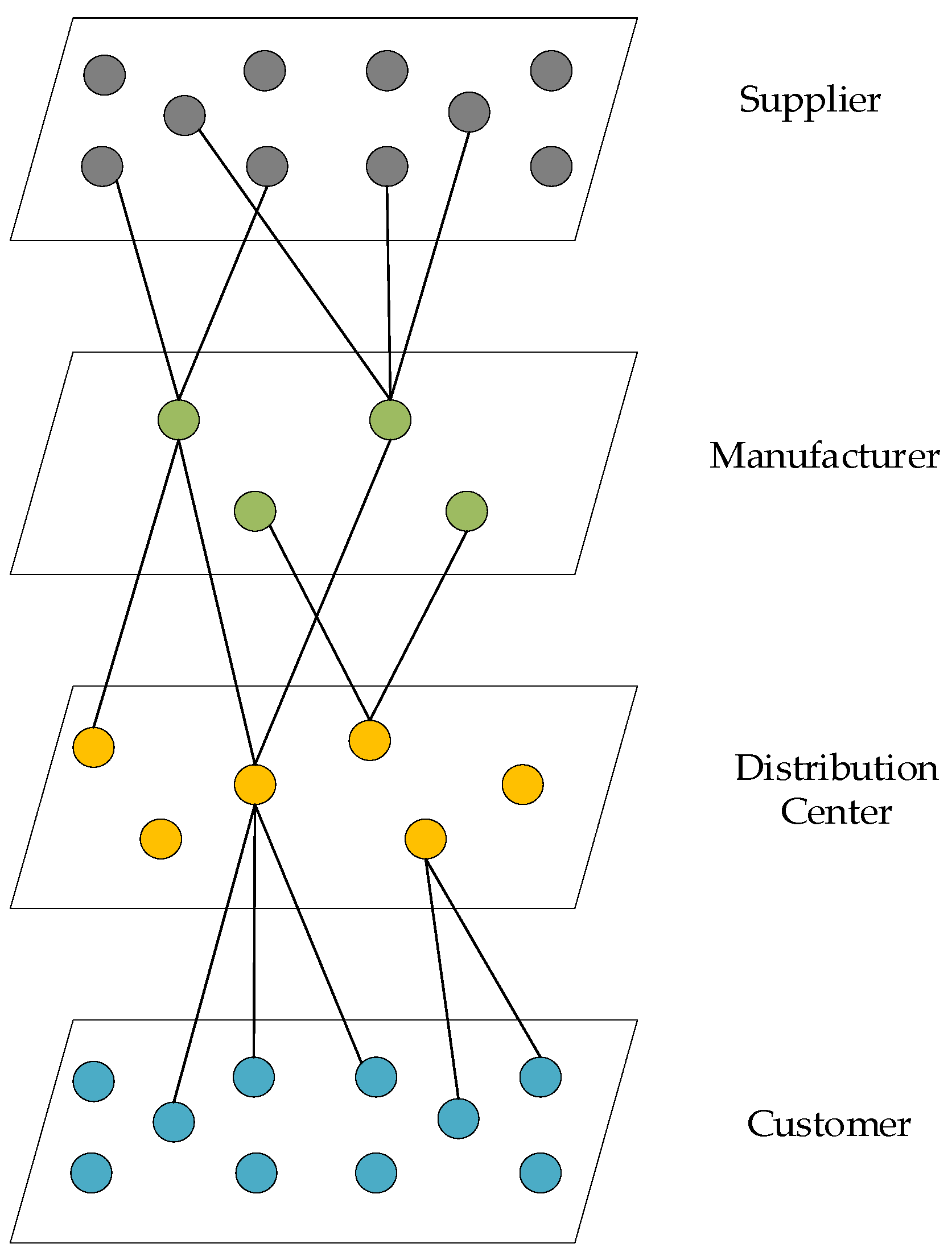
• This work considers the disruption scenario in which supply disruption and distribution center failure occur simultaneously. A two-stage stochastic programming model based on a combination of proactive and reactive defense strategies is developed to improve supply chain resilience in manufacturing companies.
• The two-stage stochastic programming model is transformed into a mixed integer linear programming (MILP) model using Latin hypercubic sampling (LHS), sample average approximation (SAA), and scenario reduction (SR) to deal with continuous demand scenarios and discrete disruptions scenarios, respectively.
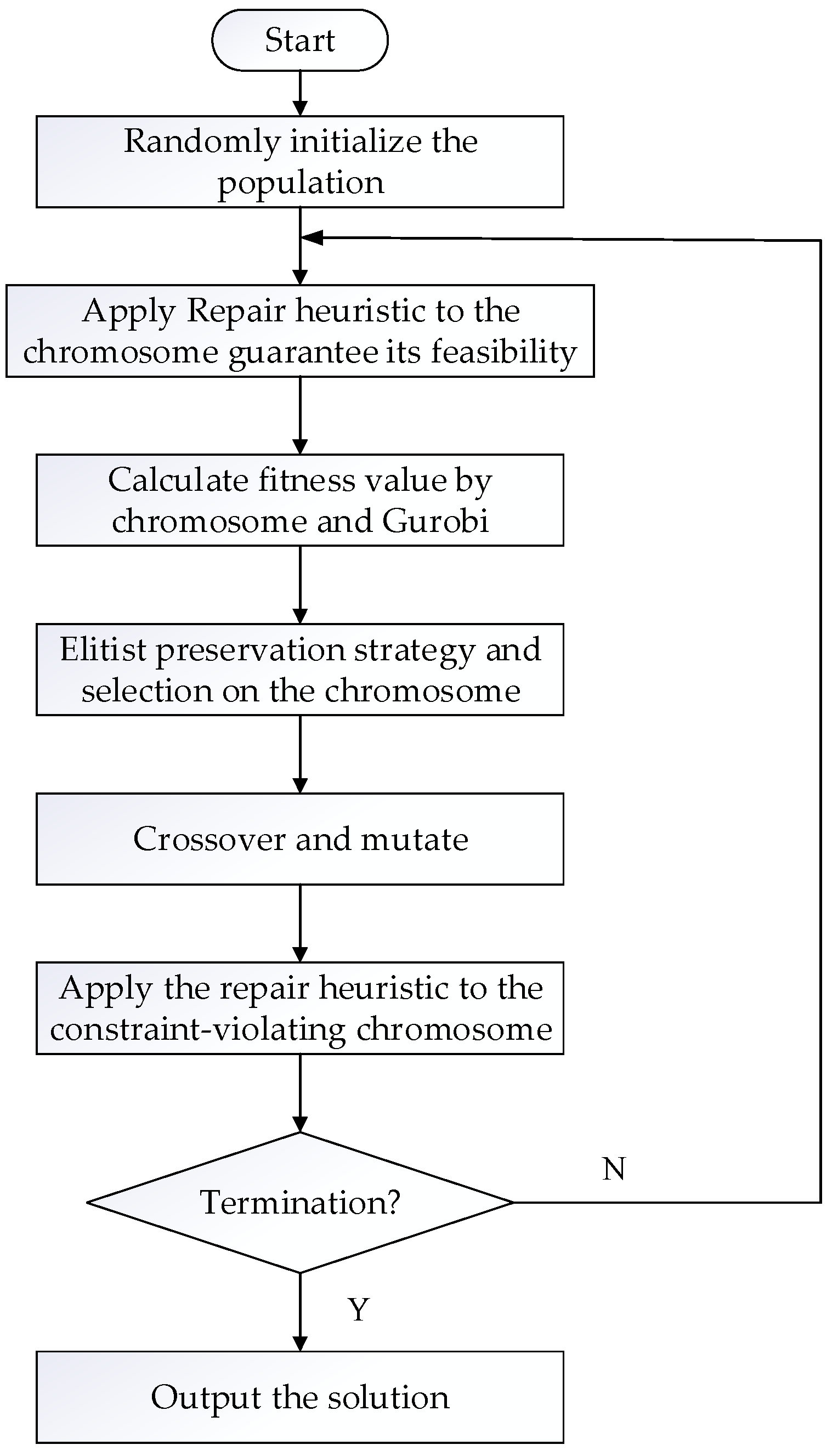
• For the model characteristics, this work develops an improved genetic algorithm combined with a heuristic algorithm to increase the efficiency of solving large-scale problems. A specific heuristic repair strategy is designed to ensure the feasibility of the solution.
• By analyzing the results, we verify the superiority of the proposed resilient strategy and algorithm in settling the supply chain disruption problem.

The remainder of this paper is organized as follows: Section 2 provides an overview of the relevant literature. The problem definition and the underlying assumptions are given in Section 3. Section 4 presents the notations and the mathematical model. Section 5 states the transformation method of the model and the proposed improved genetic algorithm. Numerical experiments and a discussion of the results are given in Section 6. Section 7 summarizes the paper and provides directions for future research.

2. Literature Review

The complexity of products, globally dispersed design, production activities, and extensive supply chains under globalization processes pose challenges for today’s enterprises. These challenges affect companies’ management of their supply chain networks and have been exacerbated by the disruptions to global supply chains caused by the COVID-19 pandemic. This situation is unprecedented, and previous studies have rarely addressed this issue directly [24].

Over the past few decades, there has been significant research on the theoretical background and key strategies of resilient supply chains to address disruption risks that may occur [25]. The literature on strategies to enhance resilience can be divided into two main aspects. One aspect is a proactive defense strategy to mitigate supply chain risks through multiple sourcing, maintaining inventory and contracting with backup suppliers [26]. Pal et al. [27] developed a three-stage supply chain model consisting of a supplier, manufacturer, and retailer to increase inventory by purchasing raw materials in advance, allowing for rapid production resumption in the event of a supply disruption. Jabbarzadeh et al. [28] proposed a stochastic bi-objective optimization model in which the two objectives were to minimize total expected costs and maximize sustainability performance. Additional production capacity, multi-source sourcing, and selection of alternate suppliers are considered in their model. Namdar et al. [29] investigated the impact of purchasing strategies such as backup supplier contracts and spot purchasing on supply chain resilience. It was found that the buyer’s early warning ability plays an important role in improving supply chain resilience. Shahed et al. [30] considered the simultaneous existence of supplier disruptions and demand uncertainty and developed a mathematical model to maximize profits by adopting an appropriate inventory policy to cope with possible disruptions in the supply chain network. Vali-Siar and Roghanian [31] proposed a multi-objective optimization model under uncertainty using multiple sourcing, enhanced infrastructure, redundant capacity, and dual-channel distribution strategies to improve supply chain resilience.

Another aspect is a reactive defense strategy to enable the supply chain to recover quickly from disruptions by developing an appropriate recovery strategy. Sawik [32] proposed a two-period modeling approach for the selection of recovery suppliers and recovery assembly plants and the decisions implemented during and after the disruption, comparing it with a multi-period approach. Paul et al. [33] considered three types of uncertain disruptions in the manufacturing supply chain: demand fluctuation, production disruption, and supply disruption, developing a quantitative model to generate a recovery plan after disruption. Khalilabadi et al. [34] developed a multi-stage stochastic planning model that uses a product substitution strategy to mitigate uncertain demand fluctuations in a multi-product supply chain. Chen et al. [35] investigated a disruption recovery strategy from a product design change and life cycle perspective and proposed a mixed integer linear programming model to solve the supply chain disruption recovery problem.

In the past, few scholars have combined proactive and reactive strategies in the design of resilient supply chains. Elluru et al. [36] proposed a location routing model that combine proactive and reactive approaches, taking into account supply chain disruptions caused by disasters. The proactive approach considered the risk factors of the facility prior to the disruption, and the reactive approach considered recovery strategies and the associated penalties. However, the long duration of the pandemic and the uncertainty about the timing and magnitude of disruptions make it necessary for enterprises to consider both pre-disruption defense strategies and post-disruption recovery strategies.

Recently, supply chain disruption recovery strategies for the pandemic have focused on the impact of disruptions on supply, production, and demand fluctuation [37]. Paul et al. [20] developed a recovery model to help enterprises for high-demand products make decisions when designing revised production schedules after supply disruptions. Nagurney et al. [38] considered the uncertainty of product demand and the impact of the COVID-19 pandemic on the workforce and developed a supply chain network optimization model to cope with supply chain disruptions. Taking into account the supply disruptions and demand fluctuations caused by the pandemic, Sawik [39] proposed a multi-portfolio approach and a scenario-based stochastic MIP model to optimize supply chain operations under ripple effects using risk mitigation inventory and alternate supplier procurement strategies. Paul et al. [40] developed a stochastic mathematical model to optimize the recovery of a three-stage supply chain with demand, supply, and capacity uncertainties due to the multi-dimensional impact of the COVID-19 pandemic.

Most existing studies have ignored the possible impact of the pandemic on facilities such as distribution centers. Distribution centers may be at risk of failing to close or not being able to meet uncertain demands. Manufacturers should consider planning backup facilities in advance or constructing temporary distribution centers if existing facilities fail. By properly locating distribution centers, the total cost of the supply chain can be reduced, and the order allocation and transportation efficiency can be improved [41,42]. Amin and Baki [43] developed a multi-objective mixed integer linear programming model for a supply chain network including multiple plants, distribution centers, demand, and products to select the best supplier and distribution center sites considering the uncertainty of demand. Jakubovskis et al. [44] proposed a robust optimization modeling method for facility location and capacity planning under uncertain demand and determined which capabilities can contribute to solution robustness through experiments. Ortiz-Astorquiza [45] conducted a review of multi-level facility location problems that extend several classical facility location problems and identified three different categories of multi-level facility location problems based on the types of decisions made in the optimization process. Saragih et al. [46] developed a heuristic method for solving the location–inventory–routing problem in a three-level supply chain system with uncertain demand. Fu et al. [47] developed a simulation-based optimization approach to the facility location and capacity planning problem under the Belt and Road initiative by considering both policy preference and customer demand uncertainties.

Table 1. Comparison between this paper and relevant studies in the literature in terms of encountered disruption and methodology.

Articles	Type of Disruption	Strategy of Resilience		Methodology
		Proactive	Reactive	Deterministic	Stochastic
Pal et al. [27]	Sd	✓		✓
Jabbarzadeh et al. [28]	Sd	✓			✓
Namdar et al. [29]	Sd	✓		✓
Shahed et al. [30]	Sd, Df	✓			✓
Vali-Siar and Roghanian [31]	Sd, Df	✓			✓
Sawik [32]	Sd, Pd		✓	✓
Paul et al. [33]	Sd, Pcu, Df		✓	✓
Khalilabadi et al. [34]	Df		✓		✓
Chen et al. [35]	Sd		✓	✓
Elluru et al. [36]	Dnf	✓	✓	✓
Paul et al. [20]	Sd		✓	✓
Nagurney et al. [38]	La		✓		✓
Paul et al. [40]	Su, Pcu, Df		✓		✓
Sawik [39]	Sd, Df	✓			✓
This paper	Sd, Dnf, Df	✓	✓		✓

Sd: supply disruption, Su: supply uncertainty, Pd: production disruption, Pcu: production capacity uncertainty, La: labor availability, Dnf: distribution network failure, Df: demand fluctuation.

summarizes the differences between this paper and related studies in the literature in terms of the types of disruptions considered and the resilience strategies employed, providing additional details to distinguish studies based on resilient supply chain optimization.

3. Problem Description and Assumptions

3.1. Problem Statement

This paper considers a four-tier supply chain network consisting of suppliers, manufacturers, distribution centers, and customers, where the distribution centers are established by the manufacturer based on the region, the number of orders, and the level of transport logistics. Nodes have a hierarchical relationship between the upstream and downstream components of the supply chain. Each layer of nodes can only be connected to its neighboring layer of nodes, and the layers of nodes are independent of each other. The supply chain network structure is shown in Figure 1. Manufacturers produce a variety of products, and each product requires a variety of parts. Different products may require the same parts, and each part is provided by one supplier. The products are first transported by the manufacturer to the distribution centers, each of which has a maximum capacity, and are then transported by the distribution center to the appropriate customers within its coverage area. Each customer’s demand for each product is uncertain.

Due to the COVID-19 pandemic, disruptions may occur in any link of the supply chain, and multiple facilities in the supply chain network may fail at the same time or one after another. Considering the ripple effect, after a disruption occurs at a certain point in the supply chain, it can spread upstream or downstream along the supply chain, leading to more large-scale failures. The propagation of disruptions in the supply chain network is shown in Figure 2, where green indicates that a node is functioning normally, yellow indicates that a node is partially disabled, red indicates that a node is completely disabled, and blue indicates that a node is affected. Here, (a) demonstrates a healthy supply chain network and (b) demonstrates disruptions occurring simultaneously at the suppliers and distribution centers, where S2 and D2 partially fail and S4 and D3 completely fail. Additionally, (c) demonstrates the supply chain network after disruption, where the productions of P1 and P2 are affected due to the failure of suppliers S2 and S4. Due to the partial failure of distribution center D2, the demands of customers C2 and C4 cannot be met. The complete failure of D3 results in an inability to handle the C5 demand, and the link between the nodes is disconnected. (d) denotes the supply chain network after considering the propagation of the disruption ripple effect. Due to the supply disruption, the production capacity of product P1 decreases and the production of product P2 is stopped. Customer C1-C4 orders for P1 may be backordered, and orders for P2 must be cancelled. All the orders for customer C5 were cancelled due to the failure of the upstream distribution center.

In order to establish a resilient supply chain network, this paper considers a combination of proactive and reactive defense strategies. The manufacturer develops appropriate raw material inventory plans and locates and constructs temporary distribution centers before disruptions occur. The objective is to determine the inventory quantities for each raw material, as well as to find a subset of temporary distribution center locations under conditions that simultaneously satisfy selection preferences, warehouse capacity, and transportation capacity constraints in order to minimize raw material inventory costs and temporary distribution center fixed costs. Considering the uncertainty of the duration of supply disruptions, the manufacturer can make design changes and partially reconfigure suppliers that cannot continue production due to supply shortages, resuming production as soon as possible. After the failure of some distribution centers, the manufacturer selects which distribution centers to open from the constructed temporary distribution centers and reconfigures the distribution network. The reconfigured supply chain network after the adoption of the recovery strategy is shown in Figure 3, where TD1 and TD2 represent the selected temporary distribution centers. When the manufacturer holds a certain amount of raw material inventory and adds AS2 as the substitute supplier for S2, P1 can fully resume production and P2 can resume partial production. In addition, NS1 is the new supplier of the new product NP1 after the design change.

This paper considers three types of disturbances that can occur in a manufacturing supply chain, namely supply disruptions, distribution center failures, and demand uncertainty, where the magnitude of supply disruptions and distribution center failures is also uncertain. These three disturbances can occur individually or simultaneously. It is difficult to obtain an accurate picture of the probability of disruption to suppliers and distribution centers as well as demand fluctuations. Manufactures can only obtain estimates from historical data. Therefore, manufacturers need to consider the following three important questions before/after disruptions:

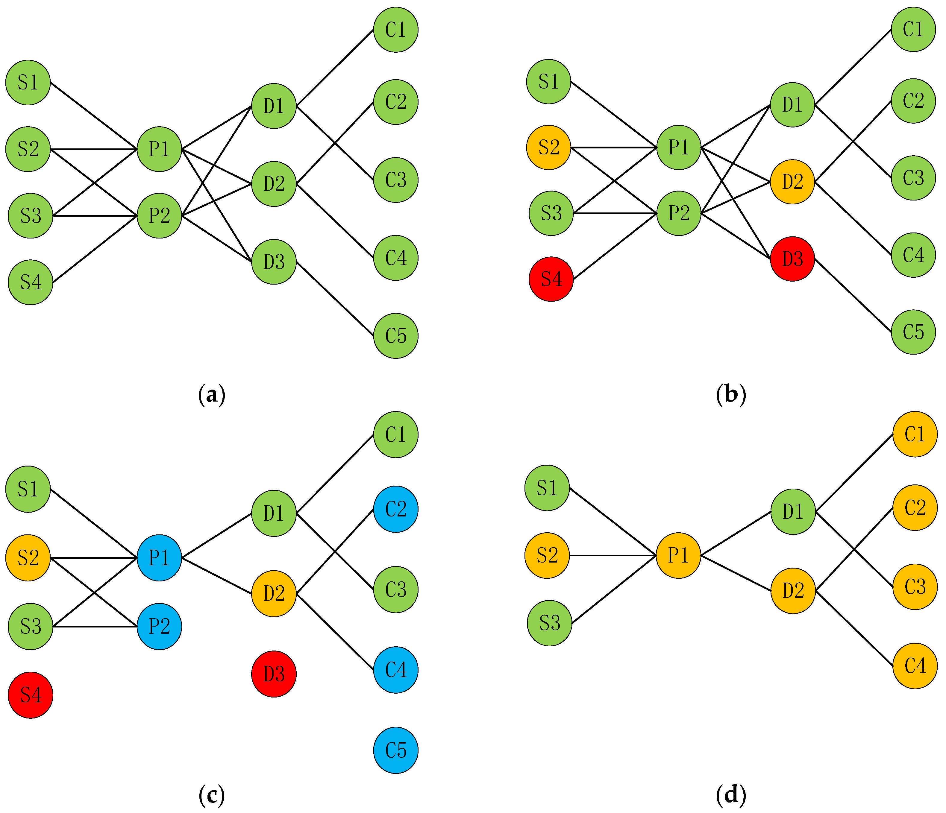
• How to determine the inventory quantity of each raw material before disruptions;
• How to locate the temporary distribution center;
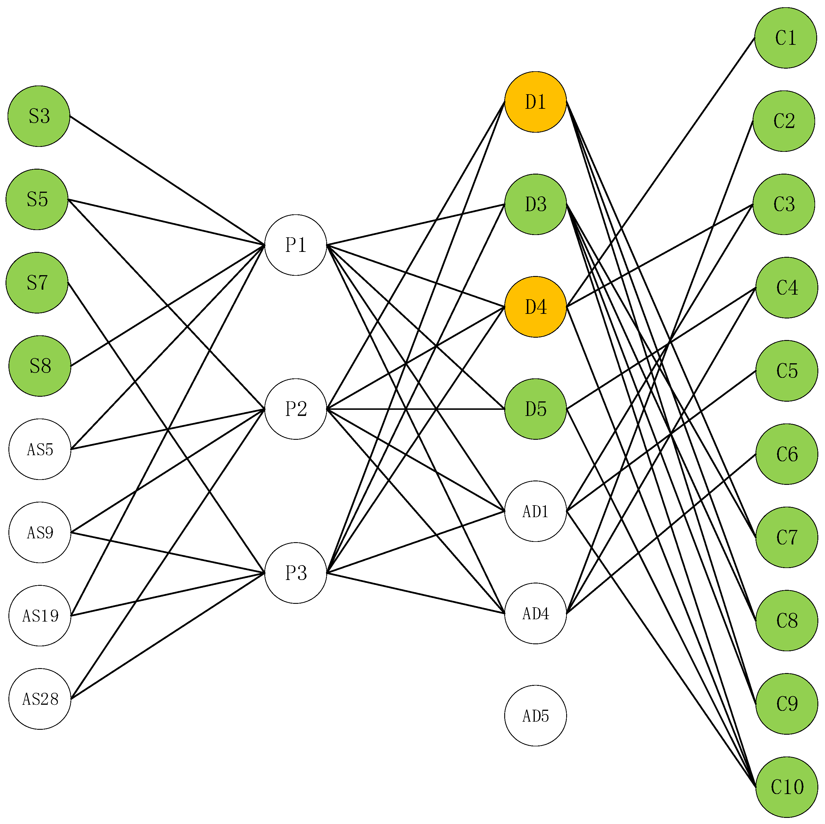
• How to choose the product change option and alternative suppliers.

3.2. Assumptions

In order to make the study more relevant and feasible, the following basic assumptions are made:

• The disruption of each supplier and distribution center is independent of each other, and the disruption may cause partial or complete failure of the facility.
• Emergency procurement needs are taken into account to consider the additional procurement cost, but the production delay caused by emergency procurement is not considered, and there is a procurement cost difference between the backup supplier and the original supplier.
• Product design changes require consideration of product design costs and new raw material procurement costs.
• The manufacturer’s preference weight coefficient for the location of the new distribution center is determined by the triangular fuzzy number $M\left(l, m,u\right)$;
• The demand of each customer for each product satisfies the normal distribution $N~\left(\mu ,{\sigma }^2\right)$, and each customer’s demand is independent of the others. When the demand of customers cannot be met due to supply shortage, the cost of sales loss will be incurred.
• Products are shipped immediately after production, regardless of storage at the manufacturer, and there are inventory capacity limitations at the distribution center.

4. Model Formulation

4.1. Notations and Decision Variables

In order to build a mathematical model, some notations are defined and listed as follows:

List of indices:

$i$	Index for original suppliers
$j$	Index for alternative suppliers
$p$	Index for products
$l$	Index for original distribution centers
$m$	Index for temporary distribution centers
$n$	Index for customers
$s$	Index for disruption scenarios

List of decision variables:

$x_{ij}^s$	1 if the part from the $i^{th}$ original supplier is changed to the raw material from the $j^{th}$ alternative supplier for the $s^{th}$ disruption scenario, else 0
$k_m$	1 if the $m^{th}$ temporary distribution center is built, else 0
$y_m^s$	1 if the $m^{th}$ temporary distribution center is used for the $s^{th}$ disruption scenario, else 0
$X_{ij}^s$	Quantity to be procured for the $s^{th}$ disruption scenario from the $j^{th}$ alternative supplier of the $i^{th}$ original supplier
$I_l$	Inventory of raw materials supplied by the $i^{th}$ original supplier
$Z_{pl}^s$	Quantity of the $p^{th}$ product transported from the manufacturer to the $l^{th}$ original distribution center for the $s^{th}$ disruption scenario
$Z_{pm}^s$	Quantity of the $p^{th}$ product transported from the manufacturer to the $m^{th}$ temporary distribution center for the $s^{th}$ disruption scenario
$Z_{pln}^s$	Quantity of the $p^{th}$ product transported from the $l^{th}$ original distribution center to the $n^{th}$ customer for the $s^{th}$ disruption scenario
$Z_{pmn}^s$	Quantity of the $p^{th}$ product transported from the $m^{th}$ temporary distribution center to the $n^{th}$ customer for the $s^{th}$ disruption scenario

List of parameters:

$u_i^s$	1 if the $i^{th}$ original supplier for the $s^{th}$ disruption scenario has not been disrupted, else 0
$v_l^s$	1 if the $l^{th}$ original distributor center for the $s^{th}$ disruption scenario has not been disrupted, else 0
$P_s$	Probability of the $s^{th}$ disruption scenario
$w_{ip}$	1 if the $i^{th}$ supplier supplies raw material for the $p^{th}$ product, else 0
$X_i$	Quantity to be procured from the $i^{th}$ original supplier
$\gamma$	Inventory as a percentage of supply
$C_i$	Unit procurement cost of raw materials from the $i^{th}$ supplier
$C_{ij}$	Unit procurement cost of raw materials from the $j^{th}$ alternative supplier of the $i^{th}$ supplier
$Q_{ij}$	Fixed change cost for the $j^{th}$ alternative supplier of the $i^{th}$ supplier
${Qc}_{ij}$	Unit production cost of changing the raw material for the product from the $i^{th}$ supplier to the $j^{th}$ alternative supplier
${Pc}_p$	Unit production cost of the $p^{th}$ product
${Is}_i$	Minimum safety stock of raw materials supplied by the $i^{th}$ original supplier
$I_{max}$	Maximum raw material inventory capacity of the manufacturer
$\mu$	Minimum percentage of inventory held by the manufacturer
${CI}_i$	Unit inventory cost of the raw materials supplied by the $i^{th}$ original supplier
$E_l$	Unit transportation cost from the manufacturer to the $l^{th}$ original distribution center
$E_m$	Unit transportation cost from the manufacturer to the $m^{th}$ temporary distribution center
$E_{ln}$	Unit transportation cost from the $l^{th}$ original distribution center to the $n^{th}$ customer
$E_{mn}$	Unit transportation cost from the $m^{th}$ temporary distribution center to the $n^{th}$ customer
$F_{np}$	Unit out-of-stock loss cost of the $p^{th}$ product order for the $n^{th}$ customer
$K_m$	Fixed cost for the $m^{th}$ temporary distribution center
$K_m^{\prime }$	Operating cost for the $m^{th}$ temporary distribution center
$A_{ij}$	Maximum capacity of the $j^{th}$ alternative supplier of the $i^{th}$ original supplier
$G_l$	Maximum capacity of the $l^{th}$ original distribution center
$H_m$	Maximum capacity of the $m^{th}$ temporary distribution center
${\tilde{D}}_{np}$	Quantity demanded by the $n^{th}$ customer for the $p^{th}$ product, which satisfies a normal distribution
$\widetilde{{\alpha }_l}$	Capacity failure coefficient of the $l^{th}$ original distribution center after a disruption
${\beta }_m$	Preference weight coefficient for the manufacturer’s preference for the $m^{th}$ candidate temporary distribution center
$\theta$	Expectation for manufacturer preference of selected locations

4.2. Model Development

It is difficult to accurately predict the probability of disruption to suppliers and distribution centers as well as demand fluctuations. For modeling and experimentation, as we assume that any supplier disruption and distribution center failure event is random, we generate disruption scenarios to determine characteristics such as the disruption size and duration. To describe disruption scenarios, A is the set consisting of all the suppliers and distribution centers, and $A_S$ is the set of all the disrupted suppliers and failure distribution centers under the disruption scenario s. If the probability of disruption of element $a$ in the set $A_S$ is $p_a$ and the elements are independent of each other, then the probability $P_s$ of the occurrence of scenario s can be calculated by the following equation [48]:

$$P_s={\prod }_{a\in A_S}{p}_a{\prod }_{a\in A\backslash A_S}\left(1-p_a\right)$$

(1)

In order to characterize the manufacturer’s preference for candidate locations, each location is associated with a preference factor, including factors such as local policy orientation, regional epidemic levels, and transportation levels, which indicate the degree of manufacturer preference for building a distribution center in that location It is difficult to know the exact selection preferences, and manufactures can only obtain estimates from managers and experts. Since the manufacturer’s preference weight coefficient $\widetilde{{\beta }_m}$ for the temporary distribution center location is somewhat fuzzy, triangular fuzzy numbers can represent the pessimistic, most likely, and optimistic values of the expert opinion. Therefore, they can be used to evaluate the manufacturer’s preference for temporary distribution centers. This paper determines the triangular fuzzy number $M\left(l, m, u\right)$ for all alternative locations through expert scoring, where m denotes the most likely preference weight coefficient for the alternative location, l and u denote the upper and lower bounds of the preference weight coefficient for the alternative location, respectively, and the graded mean integration method is used to represent the triangular fuzzy number, which transforms the manufacturer’s preference weight coefficient ${\beta }_m$ from a fuzzy number to a definite value. This can be expressed as follows:

$$G\left(\widetilde{{\beta }_m}\left(\alpha \right)\right)=\frac{{\int }_0^1\left(\frac{\alpha }{2}\right)\left[L^{-1}\left(\alpha \right)+R^{-1}\left(\alpha \right)\right]d\alpha }{{\int }_0^1\alpha d\alpha }={\int }_0^1\alpha \left[L^{-1}\left(\alpha \right)+R^{-1}\left(\alpha \right)\right]d\alpha =\frac{1}{6}(l+4m+u)$$

(2)

where $L^{-1}\left(\alpha \right)$ and $R^{-1}\left(\alpha \right)$ are the inverse functions of $L\left(\alpha \right)$ and $R\left(\alpha \right)$ (left and right function of the triangular fuzzy number), respectively, and the values of $L^{-1}\left(\alpha \right)$ and $R^{-1}\left(\alpha \right)$ are $l+(m-l)\alpha$ and $u-(u-m)\alpha$, respectively.

In order to establish a resilient supply chain network, it is necessary to not only determine the inventory plan and the construction of temporary facilities before the disruption, but also to decide the recovery plan based on the disruption scenario and the identified supply chain network. Therefore, considering both proactive and reactive defense strategies, a two-stage stochastic planning model is developed in this section. The first stage is to decide on the manufacturer’s inventory plan for each raw material and the location of the temporary distribution centers considering the manufacturer’s preference before the disruption. The second stage is to make decisions about product design changes, which temporary distribution centers will be used and their processing capacity, and delivery plans for order requirements after the disruption.

The objective function of the first stage is to maximize the total profit, which includes the cost of raw material inventory planning, the cost of temporary distribution center location construction, and the expected profit associated with disruption scenarios and stochastic demand. The first-stage model is established as follows:

$$\mathit{max} E_{\xi }R\left(x,y,X,Z,S,\xi \right)-{\sum }_{i\in I}{CI}_i{I}_i-{\sum }_{m\in M}{K}_m{k}_m$$

(3)

$$\mathrm{s}.\mathrm{t}.$$

$$I_i\le {\gamma X}_i, \forall i\in I$$

(4)

$$I_i\ge {Is}_i, \forall i\in I$$

(5)

$${\sum }_{i\in I}{I}_i\ge \mu I_{max}$$

(6)

$${\sum }_{i\in I}{I}_i\le I_{max}$$

(7)

$${\sum }_{m\in M}{\beta }_m{k}_m\ge \theta$$

(8)

$$k_m\in \left\{\mathrm{0,1}\right\}, \forall m\in M$$

(9)

$$I_{i }are positive integers, \forall i\in I$$

(10)

where $R\left(x,y,X,Z,S,\xi \right)$ denotes the expected profit associated with disruption scenarios and stochastic demand, which can be determined by the second-stage model. Constraints (4)–(7) constrain the inventory capacity of each raw material. Constraint (8) ensures the manufacturer’s preference for the selected locations for the temporary distribution centers. Constraints (9) and (10) define the range of decision variables.

The objective function of the second stage is to maximize the expected profit associated with the disruption scenario and stochastic demand, including the manufacturer’s product revenue, the manufacturer’s procurement cost from the original supplier, the product change cost, the production cost, the transportation cost from the manufacturer to the distribution centers and from the distribution centers to the customers, and the cost of lost sales. The second-stage model is established as follows:

$$\begin{gathered} R\left(x,y,X,Z,S,\xi \right)= \\ \mathit{max} {\sum }_{s\in S}{P}_s\left\{{\sum }_{p\in P}{R}_p\left({\sum }_{l\in L}{Z}_{pl}^s+{\sum }_{m\in M}{Z}_{pm}^s\right)-\left[{\sum }_{i\in I}{u}_i^s{X}_i{C}_i+{\sum }_{i\in I}{\sum }_{j\in J}\left({x_{ij}^{s}Q}_{ij}+X_{ij}^s{C}_{ij}+{X_{ij}^{s}Qc}_{ij}\right)+{\sum }_{p\in P}{Pc}_p\left({\sum }_{l\in L}{Z}_{pl}^s+{\sum }_{m\in M}{Z}_{pm}^s\right)+{\sum }_{m\in M}{K}_m^{\prime }{y}_m^s+{\sum }_{p\in P}\left({\sum }_{l\in L}{E}_l{Z}_{pl}^s+{\sum }_{m\in M}{E}_m{Z}_{pm}^s\right)+{\sum }_{n\in N}{\sum }_{p\in P}\left({\sum }_{l\in L}{E}_{ln}{Z}_{pln}^s+{\sum }_{m\in M}{E}_{mn}{Z}_{pmn}^s\right)+{\sum }_{n\in N}{\sum }_{p\in P}{F}_{np}\left({\tilde{D}}_{np}-{\sum }_{l\in L}{Z}_{pln}^s-{\sum }_{m\in M}{Z}_{pmn}^s\right)\right]\right\} \end{gathered}$$

(11)

$$\mathrm{s}.\mathrm{t}.$$

$$X_{ij}^s \le \left(1-u_i^s\right)x_{ij}^s{A}_{ij}, \forall i\in I,j\in J,s\in S$$

(12)

$${\sum }_{j\in J}{x}_{ij}^s=1-u_i^s, \forall i\in I,s\in S$$

(13)

$${u_i^{s}X}_i+{\sum }_{j\in J}{X}_{ij}^s+\left(1-u_i^s\right)I_i \ge {\sum }_{p\in P}{w}_{ip}\left({\sum }_{l\in L}{Z}_{pl}^s+{\sum }_{m\in M}{Z}_{pm}^s\right), \forall i\in I,s\in S$$

(14)

$${u_i^{s}X}_i+{\sum }_{j\in J}{X}_{ij}^s+\left(1-u_i^s\right)I_i\le {\sum }_{n\in N}{\sum }_{p\in P}{w}_{ip}{\tilde{D}}_{np},\forall i\in I, s\in S$$

(15)

$$y_m^s\le k_m, \forall m\in M,s\in S$$

(16)

$${\sum }_{m\in M}{y}_m^s\ge 1-v_l^s, \forall s\in S, l\in L$$

(17)

$${\sum }_{m\in M}{y}_m^s\le {\sum }_{l\in L}\left(1-v_l^s\right), \forall s\in S$$

(18)

$${\sum }_{p\in P}{Z}_{pl}^s \le {v_l^{s}G}_l+(1-\widetilde{{\alpha }_l})\left(1-v_l^s\right)G_l, \forall l\in L,s\in S$$

(19)

$${\sum }_{p\in P}{Z}_{pm}^s \le y_m^s{H}_m, \forall m\in M,s\in S$$

(20)

$${\sum }_{n\in N}{Z}_{pln}^s=Z_{pl}^s, \forall p\in P,l\in L,s\in S$$

(21)

$${\sum }_{n\in N}{Z}_{pmn}^s=Z_{pm}^s, \forall p\in P,m\in M,s\in S$$

(22)

$${\sum }_{l\in L}{Z}_{pln}^s+{\sum }_{m\in M}{Z}_{pmn}^s\le {\tilde{D}}_{np}, \forall p\in P,n\in N,s\in S$$

(23)

$$x_{ij}^s, y_m^s\in \left\{\mathrm{0,1}\right\}, \forall i\in I,j\in J,m\in M,s\in S$$

(24)

$$X_{ij}^s, Z_{pl}^s, Z_{pm}^s, Z_{pln}^s, Z_{pmn}^s are positive integers, \forall i\in I,j\in J,p\in P,l\in L,m\in M,n\in N,s\in S$$

(25)

where (12) indicates that the supply of the alternative suppliers must be equal to or less than their maximum supply capacity. Constraint (13) indicates that, at most, one of the alternative suppliers of the disrupted supplier has been selected. Constraints (14) and (15) ensure that the quantity of product produced by the manufacturer exceeds the amount shipped to the distribution center, but does not exceed the demand. Constraints (16)–(18) constrain which of the constructed temporary distribution centers are used. Constraints (19) and (20) indicate that the quantity of product transported from the manufacturer to the original distribution center and to the new distribution center does not exceed the handling capacity of the distribution center. Constraints (21) and (22) ensure that the quantity of each product shipped from the distribution center to the customer equals the quantity shipped by the manufacturer to the distribution center. Constraint (23) ensures that the supply of products from all the distribution centers to the customer cannot exceed the demand of this customer. Constraint (24) constrains the binary nature of the decision variables $x_{ij}^s,y_m^s$. Finally, (25) defines the other decision variables as positive integers.

5. Solution Approach

5.1. SAA and SR Method

The model developed in this paper contains fuzzy and random numbers. For the fuzzy number n, the fuzzy preference weight coefficients are transformed into a deterministic value by using the graded mean integration method to defuzzify the triangular fuzzy number in Section 4.2 through Equation (1). Since the proposed model contains uncertain demands, this paper considers Latin hypercube sampling (LHS) to obtain samples. Then, the SAA method is used to handle the uncertain demand from discrete samples rather than continuous distribution functions to approximate the expected cost [49]. Assume that ${\gamma }_1,{\gamma }_2,\dots ,{\gamma }_K$ are K uncertain demand scenarios and k is the set of demand scenarios of size K, since disruptions are difficult to describe using continuous probability distribution functions and the probability of each disruption scenario is different. Therefore, for discrete disrupted scenarios, the scenario reduction (SR) method can be adopted to reduce the number of disruption scenarios [50]. The main idea of the SR method is to select a subset from the full set of scenarios, reduce the number of scenarios, and minimize the difference between the optimal objective function value of the full scenario problem and the optimal objective function value of the reduced scenario problem. Using the SAA and SR method, the two-stage stochastic planning model can be rewritten as a deterministic MILP model as follows:

$$\mathit{max} \frac{1}{K}{\sum }_{k\in K}\left\{{\sum }_{s\in \widehat{S}}\widehat{p_s}\left[{\sum }_{p\in P}{R}_p\left({\sum }_{l\in L}{Z}_{plk}^s+{\sum }_{m\in M}{Z}_{pmk}^s\right)-{\sum }_{i\in I}{u}_i^s{X}_i{C}_i-{\sum }_{i\in I}{\sum }_{j\in J}\left({x_{ijk}^{s}Q}_{ij}+X_{ijk}^s{C}_{ij}+{X_{ijk}^{s}Qc}_{ij}\right)-{\sum }_{p\in P}{Pc}_p\left({\sum }_{l\in L}{Z}_{plk}^s+{\sum }_{m\in M}{Z}_{pmk}^s\right)-{\sum }_{m\in M}{K}_m^{\prime }{y}_{mk}^s-{\sum }_{p\in P}\left({\sum }_{l\in L}{E}_l{Z}_{plk}^s+{\sum }_{m\in M}{E}_m{Z}_{pmk}^s\right)-{\sum }_{n\in N}{\sum }_{p\in P}\left({\sum }_{l\in L}{E}_{ln}{Z}_{plnk}^s+{\sum }_{m\in M}{E}_{mn}{Z}_{pmnk}^s\right)-{\sum }_{n\in N}{\sum }_{p\in P}{F}_{np}\left(D_{npk}-{\sum }_{l\in L}{Z}_{plnk}^s-{\sum }_{m\in M}{Z}_{pmnk}^s\right)\right]\right\}-{\sum }_{i\in I}{CI}_i{I}_i-{\sum }_{m\in M}{K}_m{k}_m$$

(26)

$$\mathrm{s}.\mathrm{t}.$$

$$X_{ijk}^s \le \left(1-u_i^s\right)x_{ijk}^s{A}_{ij}, \forall i\in I,j\in J,s\in S, k\in K$$

(27)

$${\sum }_{j\in J}{x}_{ijk}^s=1-u_i^s, \forall i\in I,s\in S,k\in K$$

(28)

$$I_i\le {\gamma X}_i, \forall i\in I$$

(29)

$$I_i\ge {Is}_i, \forall i\in I$$

(30)

$${\sum }_{i\in I}{I}_i\ge \mu I_{max}$$

(31)

$${\sum }_{i\in I}{I}_i\le I_{max}$$

(32)

$${u_i^{s}X}_i+{\sum }_{j\in J}{X}_{ijk}^s+\left(1-u_i^s\right)I_i\ge {\sum }_{p\in P}{w}_{ip}\left({\sum }_{l\in L}{Z}_{plk}^s+{\sum }_{m\in M}{Z}_{pmk}^s\right), \forall i\in I,s\in S, k\in K$$

(33)

$${u_i^{s}X}_i+{\sum }_{j\in J}{X}_{ijk}^s+\left(1-u_i^s\right)I_i\le {\sum }_{n\in N}{\sum }_{p\in P}{w}_{ip}{D}_{npk},\forall i\in I, s\in S, k\in K$$

(34)

$${\sum }_{m\in M}{\beta }_m{k}_m\ge \theta$$

(35)

$$y_{mk}^s\le k_m, \forall m\in M,s\in S,k\in K$$

(36)

$${\sum }_{m\in M}{y}_{mk}^s\ge 1-v_l^s, \forall s\in S, l\in L,k\in K$$

(37)

$${\sum }_{m\in M}{y}_{mk}^s\le {\sum }_{l\in L}\left(1-v_l^s\right), \forall s\in S,k\in K$$

(38)

$${\sum }_{p\in P}{Z}_{plk}^s\le {v_l^{s}G}_l+\left(1-\widetilde{{\alpha }_l}\right)\left(1-v_l^s\right)G_l, \forall l\in L,s\in S, k\in K$$

(39)

$${\sum }_{p\in P}{Z}_{pmk}^s\le y_m^s{H}_m, \forall m\in M,s\in S, k\in K$$

(40)

$${\sum }_{n\in N}{Z}_{plnk}^s=Z_{plk}^s, \forall p\in P,l\in L,s\in S, k\in K$$

(41)

$${\sum }_{n\in N}{Z}_{pmnk}^s=Z_{pmk}^s, \forall p\in P,m\in M,s\in S, k\in K$$

(42)

$${\sum }_{l\in L}{Z}_{plnk}^s+{\sum }_{m\in M}{Z}_{pmnk}^s\le D_{npk}, \forall p\in P,n\in N,s\in S, k\in K$$

(43)

$$k_m,x_{ijk}^s, y_{mk}^s\in \left\{\mathrm{0,1}\right\}, \forall i\in I,j\in J,m\in M,s\in S,k\in K$$

(44)

$$I_{i },X_{ijk}^s, Z_{plk}^s, Z_{pmk}^s, Z_{plnk}^s, Z_{pmnk}^s are positive integers, \forall i\in I,j\in J,p\in P,l\in L,m\in M,n\in N,s\in S, k\in K$$

(45)

where $\widehat{S}$ and $\widehat{p_s}$ denote the set of new disruption scenarios and the corresponding probability of disruption occurrence after descending the disruption scenario.

5.2. Improved Genetic Algorithm

The proposed problem of alternative supplier selection and temporary distribution center location is very complex, which is NP-hard by nature. Various optimization tools have been widely used to solve similar small- and medium-sized problems, although there are limitations in terms of long solution times and the size of the solutions. This requires the development of an efficient and effective optimization algorithm to find the optimal or approximate optimal solution [51]. Genetic algorithms are stochastic global search optimization methods whose computational mechanisms are derived from natural selection and natural adaptation processes. Therefore, considering that the model processed using the SAA and SR methods is MILP with constraints, an improved genetic algorithm is developed in this paper as a solution to determine the optimal value. The algorithm adopts a number of effective strategies to solve the problem by targeting the repair heuristics for the specific problem of the proposed model to improve the solving power of the algorithm.

The components of a chromosome are encoded in segments. The first part determines the selection options for alternative suppliers after product design changes for each disruption scenario using integer coding. The second part indicates the quantity of each raw material in stock using integer coding. The third part determines the location of the temporary distribution center and is binary coded.

Since it is not easy to randomly generate raw material inventory quantities that satisfy the manufacturer’s inventory capacity constraints and demand constraints as feasible chromosomes, a specific repair heuristic is developed to ensure the feasibility of the solution represented by the chromosome. The repair heuristic is presented as follows:

Step 1: Calculate the sum of the inventory of each raw material. If it exceeds the manufacturer’s maximum inventory capacity, proceed to step 2, otherwise proceed to step 3.

Step 2: Count the number $b_i$ of disruptions for each supplier in all the disruption situations S and calculate the maximum inventory of each raw material as $B_i=I_{max}\times (b_i/{\sum }_{i\in I}{b}_i)$. If the inventory of the $i^{th}$ raw material exceeds $B_i$, it will be changed to $B_i$, otherwise it will remain unchanged.

Step 3: If the total inventory of raw materials is less than $\mu I_{max}$, first calculate $b_i/{\sum }_{i\in I}{b}_i$ to sort from largest to smallest, and then increase the inventory of each raw material in order until the requirement is satisfied, otherwise it will remain unchanged.

After generating the alternative supplier solution $x_{ij}^s$ after the product change and the original raw material inventory $I_i$ by chromosome, a heuristic strategy is designed to obtain the procurement quantity of each alternative raw material according to the customer’s demand for each product under a disruption scenario. The heuristic strategy is presented as follows:

Step 1: Determine the current disruption scenario s, if $u_i=0$ and $x_{ij}=1$, calculate $X_{ij}={\sum }_{n\in N}{\sum }_{p\in P}{w}_{ip}{D}_{npk}-I_i$, otherwise $X_{ij}=0$.

Step 2: In order to avoid the calculated $X_{ij}$ violating the supply capacity limit $A_{ij}$ of the selected alternative supplier, if $X_{ij}>A_{ij}$, $X_{ij}=A_{ij}$, otherwise $X_{ij}$ remains unchanged.

In the evaluation process, the objective function of maximizing the manufacturer’s profit is used as the fitness function. The part of the function related to the decision variables contained in the generated chromosome can be calculated directly. The remaining part of the function is related to the quantity of raw materials purchased by the manufacturer, and the allocation of orders between the manufacturer, distribution centers, and retailers can be formulated as an integer programming problem determined through optimization using Gurobi. The procedures of the improved genetic algorithm are presented in Figure 4.

6. Numerical Experiments

This section verifies the feasibility of the proposed model and the validity of the proposed genetic algorithm through numerous examples. The parameters are determined based on the assumptions made for the model, and values are assigned to each parameter through a randomly generated data set. In addition, we perform a sensitivity analysis on the different parameters to characterize the effect of their changes on the results.

6.1. Computational Results

It is assumed that eight suppliers provide raw materials for the manufacturer, and the manufacturer produces three products, each of which requires a different combination of raw materials. The products will first be shipped from the manufacturer to the distribution center and then distributed to the customers according to their orders. There are five distribution centers that deliver orders to ten customers, and the distribution areas can overlap. After the supply disruption, five alternative suppliers are available for each raw material that needs to be changed, and their maximum supply capacity is required to meet the raw material quantity required for the production of the product. There are six temporary distribution center locations to be selected, taking into account the manufacturer’s selection preferences and the new distribution center capacity constraints. The parameters of each part of the supply chain are determined based on the assumptions made for the model and are generated randomly within the range of values.

Table 2. Supplier parameters.

Supplier	Alternative Supplier	${\mathit{B}}_{\mathit{i}\mathit{j}}$	${\mathit{Q}}_{\mathit{i}\mathit{j}}$	${\mathit{C}}_{\mathit{i}\mathit{j}}$
S1	AS1–AS5	(19,500, 21,500)	(10,000, 13,500)	(3, 5)
S2	AS6–AS10	(20,000, 21,500)	(12,500, 15,000)	(2, 4)
S3	AS11–AS15	(9100, 9350)	(10,000, 13,000)	(4, 5)
S4	AS16–AS20	(19,500, 21,500)	(12,500, 14,500)	(3, 5)
S5	AS21–AS25	(19,500, 21,000)	(10,500, 12,000)	(2, 3)
S6	AS26–AS30	(20,500, 22,000)	(11,500, 13,500)	(3, 4)
S7	AS31–AS35	(10,500, 12,000)	(10,000, 11,500)	(4, 5)
S8	AS36–AS40	(9100, 9350)	(11,000, 13,500)	(2, 4)

presents the range of values for the parameter information of the alternative suppliers.

The range of values for the parameters related to manufacturer selection preference, capacity, and fixed cost of the temporary distribution centers are shown in

Table 3. Temporary distribution center parameters.

Distribution Center	${\mathit{K}}_{\mathit{m}}$	${\mathit{H}}_{\mathit{m}}$	Selection Preference
TD1	15,000	5900	(0.25, 0.30, 0.35)
TD2	16,000	6250	(0.2, 0.32, 0.56)
TD3	14,000	6000	(0.06, 0.1, 0.2)
TD4	12,500	6400	(0.04, 0.2, 0.3)
TD5	15,500	6150	(0.25, 0.45, 0.65)
TD6	17,000	6000	(0.16, 0.24, 0.28)

.

Table 4. Customer parameters.

Product	P1		P2		P3
Customer	${\mathit{\mu }}_{\mathit{n}1}$	${\mathit{\sigma }}_{\mathit{n}1}^2$	${\mathit{\mu }}_{\mathit{n}2}$	${\mathit{\sigma }}_{\mathit{n}2}^2$	${\mathit{\mu }}_{\mathit{n}3}$	${\mathit{\sigma }}_{\mathit{n}3}^2$
C1–C10	(800, 1000)	(60, 100)	(900, 1100)	(80, 120)	(900,1200)	(70, 150)

presents the parameter information of the customers’ demand.

The numerical experiments assume different supplier disruptions as well as distribution center failures to demonstrate the validity of the proposed model of alternative supplier selection considering product design changes, as well as temporary distribution center location considering manufacturer selection preferences. In each disruption scenario, the combination of disrupted suppliers and failed distribution centers is different, and the disrupted suppliers and failed distribution centers are independent of each other. Considering the huge number of disruption scenarios generated by different supplier and distribution center combinations, we use the SR method to reduce the number of disruption scenarios and select typical samples of disruption scenarios to test the results of the problem to validate the proposed model and the improved genetic algorithm.

The disruption scenarios after the scenario reduction are shown in

Table 5. Disruption scenarios after the SR.

Supplier	Distribution Center	Disruption Scenarios	Disruption Scenario after SR Method
8	5	8192	(1,1,1,1,1,1,1,1|1,1,1,1,1), (0,0,0,0,0,0,0,0|0,0,0,0,0), (0,0,1,0,1,0,1,1|0,0,1,0,1), (0,0,1,0,0,0,0,1|0,0,1,0,0), (1,1,1,0,1,1,1,1|0,0,1,0,1), (1,1,1,0,1,1,1,1|1,1,1,0,1)

. Based on the results in Table 5, we can determine that the 8192 disruption scenarios are reduced to 6 scenarios, which demonstrates that the SR method is effective.

Table 6. The results under different supply chain states.

State of Supply Chain	Total Profit	Temporary Distribution Center
Normal operation	548,798	—
Without any measure	186,624	—
Proposed resilient strategy	315,161	TD1, TD4, TD5

shows the manufacturer’s total profit when the supply chain is functioning normally, the expected profit of the manufacturer in the presence of disruption without considering the resilient strategy, and the results of the manufacturer’s solution using holding inventory before disruption, establishing temporary distribution centers, and using a product design change strategy after disruption. The optimization results show that by formulating a reasonable inventory plan, determining the location of the temporary distribution centers before disruptions, and selecting a reasonable product change plan for the raw materials when disruptions occur, the supply chain resilience can be improved, and the losses caused by disruptions to the supply chain can be reduced.

Table 7. Optimization results under different disruption scenarios.

Case	Disruption Scenario	Total Profit	Alternative Supplier Options	Distribution Center Options
1	(1,1,1,1,1,1,1,1|1,1,1,1,1)	388,122	—	—
2	(0,0,0,0,0,0,0,0|0,0,0,0,0)	−71,626	AS5, AS9, AS15, AS19, AS24, AS28, AS33, AS37	TD1, TD4, TD5
3	(0,0,1,0,1,0,1,1|0,0,1,0,1)	224,590	AS5, AS9, AS19, AS28	TD1, TD4
4	(0,0,1,0,0,0,0,1|0,0,1,0,0)	163,221	AS5, AS9, AS19, AS24, AS28, AS33,	TD1, TD4, TD5
5	(1,1,1,0,1,1,1,1|0,0,1,0,1)	409,376	AS19	TD1, TD4
6	(1,1,1,0,1,1,1,1|1,1,1,0,1)	418,586	AS19	TD4

shows the manufacturer’s maximum profit under different disruption scenarios and disruption recovery plans after adopting a proactive defense strategy, developing an inventory plan, and identifying temporary distribution center locations.

Figure 5 gives the results of the supply chain reconfiguration optimization in the disruption scenario of Case 3. The original suppliers S1, S2, S4, and S6 were disrupted, and the production of products P1, P2, P3 are affected. By incorporating design changes for the disrupted raw materials, AS5, AS9, AS19, and AS28 are selected as new suppliers and a new supply network is established. Considering the manufacturer’s selection preference as well as the handling capacity and construction cost of the temporary distribution center, TD1, TD4, and TD5 are identified as temporary distribution centers. Due to the pandemic, the original distribution centers D1, D2 and D4 failed at the same time. Considering the failure situation and customer demands, the temporary distribution centers TD1 and TD4 are opened. Taking the maximum total profit as the objective, the production, transportation, and distribution plans of the reconstructed supply chain network are determined.

In order to validate the performance of the proposed improved genetic algorithm, we conducted extensive numerical experiments on test problems with randomly generated data for different sizes of suppliers, product types, distribution centers, and customers. For small-scale problems, the proposed genetic algorithm has similar performance in terms of the approximate optimal solutions obtained compared to Gurobi, and high-quality solutions can be found for small-scale problems. When the problem size is larger, although the quality of the solution obtained by the proposed genetic algorithm decreases, it is still within the acceptable range of error. In addition, for the proposed stochastic programming model, Gurobi is unable to find a solution to the problem after running for a long time, as the disruption scenario and the sampling samples have increased. In

Table 8. Results of Gurobi and the proposed genetic algorithm.

Instance	Supplier	Distribution Center	Customer	Disruption Scenario	Sample	$\frac{{\mathit{T}\mathit{C}}_{\mathit{G}\mathit{A}}-{\mathit{T}\mathit{C}}_{\mathit{G}\mathit{u}\mathit{r}\mathit{o}\mathit{b}\mathit{i}}}{{\mathit{T}\mathit{C}}_{\mathit{G}\mathit{u}\mathit{r}\mathit{o}\mathit{b}\mathit{i}}}$
1	8	5	10	6	10	0.023
2					30	0.021
3					50	0.025
4		10	25	8	10	0.032
5					30	0.036
6					50	0.038
7	12	5	10	8	10	0.045
8					30	0.05
9					50	0.048
10		10	25	9	10	0.054
11					30	0.049
12					50	*
13	16	5	10	9	10	0.076
14					30	0.072
15					50	*
16		10	25	10	10	0.082
17					30	*
18					50	*

* Gurobi cannot locate the solution to the problem after running for a long time.

, the optimality gap between the optimal solution obtained using the proposed algorithm and the optimal solution obtained using Gurobi is illustrated.

6.2. Sensitivity Analysis

The manufacturer’s total profit varies with different parameters. In this section, a sensitivity analysis is performed to illustrate the effects of various parameters on the expected profit of the proposed resilient supply chain. $I_{max}$ and $H_m$ are important parameters in the formulation of a proactive defense strategy, and $Q_{ij}$ is an important parameter for determining the raw material change plan and selecting alternative suppliers after disruption. We examine the sensitivity of the objective function value with respect to changing these pricing parameters. To characterize the impact, a sensitivity analysis is performed for different parameters. Only one parameter is changed for each analysis, and the remainder are kept the same as in Section 6.1. We change the parameters to −50%, −25%, +25%, +50%, and +75% of the original value to solve for the result.

Figure 6 shows the variation in the manufacturer’s expected total profit with the maximum raw material inventory capacity. It can be seen that as the maximum inventory capacity increases, the expected profit also increases. However, when the capacity increases to a certain value, profits no longer change. As the capacity continues to increase, the profit decreases due to redundancy.

Figure 7 shows the variation in the manufacturer’s total profit with the capacity of the temporary distribution center. When the other parameters are fixed, the expected profit of the manufacturer increases as the capacity of the temporary distribution center increases. The manufacturer’s expected profit is more sensitive to the capacity of the temporary distribution center, and small changes in the parameter values can quickly change the resultant values. When it increases to a certain value, the profit tends to be constant. Therefore, it is necessary to plan the capacity of the temporary distribution center when selecting its location. Figure 8 shows the variation in the manufacturer’s total profit with the cost of product change. It can be seen that the total profit decreases as the product change cost increases.

6.3. Managerial Insights

This paper considers a four-tier supply chain with uncertain demand. When the supply chain faces supply disruptions and the distribution center failures due to the pandemic, the manufacturer adopts a combination of proactive and reactive strategies. Mitigation and recovery decisions to improve supply chain resilience include raw material mitigation inventories and temporary distribution center locations before disruptions, as well as emergency sourcing and product changes after disruptions. This work can be used in a wide range of manufacturing industries to effectively reduce losses in the manufacturing supply chain in the event of supply disruptions and distribution center failures. This work is also applicable to changes in product and distribution networks caused by changes in demand. Our research can provide managers with the following insights:

• The computational results show that a combination of proactive and reactive resilience strategies can significantly improve expected profits under pandemic disruptions and ripple effects. The proposed model can help managers consider factors such as market demand, distribution center capacity, and the supply situation in the decision process of designing a resilient supply chain to cope with unexpected disruptions similar to those caused by a pandemic.
• The first stage of the model can help manufacturers effectively set mitigation inventory and the location of temporary distribution centers to compensate for possible supply shortages and existing distribution center failures in the event of pandemic disruptions, avoiding greater losses. To reduce the cost of redundancy, managers should reasonably plan inventory capacity and temporary distribution center capacity.
• The second-stage model can help managers make decisions about the product design change plan and the selection of alternative suppliers, as well as product transportation and delivery plans, taking into account the cost of product change and the sale loss caused by it, as well as the compensation cost for failing to deliver to customers on time and other factors.
• The improved genetic algorithm developed in this paper can help decision-makers to quickly assess the impact of different measures in response to the risk of a potential pandemic disruptions under different disruption scenarios in the future.

7. Conclusions

This paper investigates a resilient supply chain disruption recovery problem with the context of the COVID-19 pandemic, which considers a supply chain network with supply disruptions and distribution center failure risks, as well as the presence of demand fluctuations, adopting a make-to-order approach. A mathematical model is developed based on raw material inventory management and temporary distribution center location before disruption, and a product design change strategy is developed after the disruption with the objective of maximizing the manufacturer’s profit. The two-stage stochastic programming model with demand uncertainty is approximated as an MILP model using SAA and LHS methods. To overcome the impact of a large number of disruption scenarios on the solution of the MILP model, SR is used to select representative disruption scenarios among them. First, a small-scale numerical example is given to illustrate the problem of selecting alternative suppliers, developing an integrated production plan and locating temporary distribution centers in the disruption scenario. The numerical experiment shows that the proposed model is effective in reducing the manufacturer’s losses in the case of supply chain disruption. In addition, to efficiently solve large-sized problems, an improved genetic algorithm is proposed. Then, extensive numerical experiments are conducted using randomly generated test problems of different sizes. The results show that the proposed genetic algorithm has similar performance to Gurobi in finding the approximate optimal solution and can obtain a high-quality solution within the acceptable error range.

There are still issues in this paper that deserve further research and discussion. Firstly, we will consider a more realistic multi-product supply chain network and consider the impact of third-party distribution centers. Secondly, this work can be extended to multi-stage stochastic programming and the design of algorithms to obtain high quality solutions. Thirdly, considering the influence of the relationships between each link of the supply chain and the optimization results can be another research direction in the future.

References

1. Chowdhury, M.T.; Sarkar, A.; Paul, S.K.; Moktadir, M.A. COVID-19 pandemic related supply chain studies: A systematic review. Transp. Res. Logist. Transp. Rev. 2021, 148, 102271. [Google Scholar] [CrossRef] [PubMed]
2. Salama, M.R.; McGarvey, R.G. Resilient supply chain to a global pandemic. Int. J. Prod. Res. 2023, 61, 2563–2593. [Google Scholar] [CrossRef]
3. Kim, S.H.; Tomlin, B. Guilt by association: Strategic failure prevention and recovery capacity investments. Manag. Sci. 2013, 59, 1631–1649. [Google Scholar] [CrossRef]
4. Ozdemir, D.; Sharma, M.; Dhir, A.; Daim, T. Supply chain resilience during the COVID-19 pandemic. Technol. Soc. 2022, 68, 101847. [Google Scholar]
5. Ivanov, D. Predicting the impacts of epidemic outbreaks on global supply chains: A simulation-based analysis on the coronavirus outbreak (COVID-19/SARS-CoV-2) case. Transp. Res. Logist. Transp. Rev. 2020, 136, 101922. [Google Scholar] [CrossRef] [PubMed]
6. Ivanov, D.; Sokolov, B.; Dolgui, A. The ripple effect in supply chains: Trade-off ‘efficiency-flexibility-resilience’ in disruption management. Int. J. Prod. Res. 2014, 52, 2154–2172. [Google Scholar] [CrossRef]
7. Li, Y.; Chen, K.; Collignon, S.; Collignon, S.; Ivanov, D. Ripple effect in the supply chain network: Forward and backward disruption propagation, network health and firm vulnerability. Eur. J. Oper. Res. 2021, 291, 1117–1131. [Google Scholar] [CrossRef]
8. Ramani, V.; Ghosh, D.; Sodhi, M.S. Understanding systemic disruption from the COVID-19-induced semiconductor shortage for the auto industry. Omega 2022, 113, 102720. [Google Scholar] [CrossRef]
9. Paul, S.K.; Chowdhury, P.; Chowdhury, M.T.; Chakrabortty, R.K.; Moktadir, M.A. Operational challenges during a pandemic: An investigation in the electronics industry. Int. J. Logist. Manag. 2023, 34, 336–362. [Google Scholar] [CrossRef]
10. Rajesh, R. Flexible business strategies to enhance resilience in manufacturing supply chains: An empirical study. J. Manuf. Syst. 2021, 60, 903–919. [Google Scholar]
11. El, B.J.; Ruel, S. Can supply chain risk management practices mitigate the disruption impacts on supply chains’ resilience and robustness? Evidence from an empirical survey in a COVID-19 outbreak era. Int. J. Prod. Econ. 2021, 233, 2–51. [Google Scholar]
12. Wang, J.W.; Muddada, R.R.; Wang, H.F.; Ding, J.L.; Lin, Y.Z.; Liu, C.L.; Zhang, W.J. Toward a resilient holistic supply chain network system: Concept, review and future direction. IEEE Syst. J. 2016, 10, 410–421. [Google Scholar] [CrossRef]
13. Lucker, F.; Seifert, R.W.; Bicer, I. Roles of inventory and reserve capacity in mitigating supply chain disruption risk. Int. J. Prod. Res. 2019, 57, 1238–1249. [Google Scholar] [CrossRef]
14. Feng, X.H.; He, Y.C.; Kim, K.H. Space planning considering congestion in container terminal yards. Transp. Res. Methodol. 2022, 158, 52–77. [Google Scholar] [CrossRef]
15. Yang, D.; Pan, K.; Wang, S. On service network improvement for shipping lines under the one belt one road initiative of China. Transp. Res. Logist. Transp. Rev. 2018, 117, 82–95. [Google Scholar] [CrossRef]
16. Lee, P.T.W.; Hu, Z.H.; Lee, S.; Feng, X.H.; Notteboom, T. Strategic locations for logistics distribution centers along the Belt and Road: Explorative analysis and research agenda. Transp. Policy 2022, 116, 24–47. [Google Scholar] [CrossRef]
17. Liu, Y.; Ma, X.X.; Qiao, W.L.; Han, B. A methodology to model the evolution of system resilience for Arctic shipping from the perspective of complexity. Marit. Policy Manag. 2023. [CrossRef]
18. Panahi, R.; Afenyo, M.; Ng, A.K.Y. Developing a resilience index for safer and more resilient arctic shipping. Marit. Policy Manag. 2023, 50, 861–875. [Google Scholar] [CrossRef]
19. Ivanov, D.; Dolgui, A.; Sokolov, B.; Ivanova, M. Literature review on disruption recovery in the supply chain. Int. J. Prod. Res. 2017, 55, 6158–6174. [Google Scholar] [CrossRef]
20. Paul, S.K.; Chowdhury, P. A production recovery plan in manufacturing supply chains for a high-demand item during COVID-19. Int. J. Phys. Distrib. Logist. Manag. 2021, 51, 104–125. [Google Scholar] [CrossRef]
21. Hishamuddin, H.; Sarker, R.; Essam, D. A disruption recovery model for a single stage production inventory system. Eur. J. Oper. Res. 2012, 222, 464–473. [Google Scholar] [CrossRef]
22. Paul, S.K.; Sarker, R.; Essam, D. A reactive mitigation approach for managing supply disruption in a three-tier supply chain. J. Intel. Manuf. 2018, 29, 1581–1597. [Google Scholar] [CrossRef]
23. Chen, J.Z.; Wang, H.F.; Zhong, R.Y. A supply chain disruption recovery strategy considering product change under COVID-19. J. Manuf. Syst. 2021, 60, 920–927. [Google Scholar] [CrossRef]
24. Ivanov, D. Viable supply chain model: Integrating agility, resilience and sustainability perspectives-lessons from and thinking beyond the COVID-19 pandemic. Ann. Oper. Res. 2020. [CrossRef]
25. Tukamuhabwa, B.R.; Stevenson, M.; Busby, J.; Zorzini, M. Supply Chain Resilience: Definition, Review and Theoretical Foundations for Further Study. Int. J. Prod. Res. 2015, 53, 5592–5623. [Google Scholar] [CrossRef]
26. Torabi, S.A.; Baghersad, M.; Mansouri, S.A. Resilient Supplier Selection and Order Allocation Under Operational and Disruption Risks. Transp. Res. Part E Logist. Transp. Rev. 2015, 79, 22–48. [Google Scholar] [CrossRef]
27. Pal, B.; Sana, S.S.; Chaudhuri, K. A multi-echelon production–inventory system with supply disruption. J. Manuf. Syst. 2014, 33, 262–276. [Google Scholar] [CrossRef]
28. Jabbarzadeh, A.; Fahimnia, B.; Sabouhi, F. Resilient and sustainable supply chain design: Sustainability analysis under disruption risks. Int. J. Prod. Res. 2018, 56, 5945–5968. [Google Scholar] [CrossRef]
29. Namdar, J.; Li, X.P.; Sawhney, R.; Pradhan, N. Supply chain resilience for single and multiple sourcing in the presence of disruption risks. Int. J. Prod. Res. 2018, 56, 2339–2360. [Google Scholar] [CrossRef]
30. Shahed, K.S.; Azeem, A.; Ali, S.M.; Moktadir, M.A. A supply chain disruption risk mitigation model to manage COVID-19 pandemic risk. Environ. Sci. Pollut. Res. 2021. [Google Scholar] [CrossRef]
31. Vali-Siar, M.M.; Roghanian, E. Sustainable, resilient and responsive mixed supply chain network design under hybrid uncertainty with considering COVID-19 pandemic disruption. Sustain. Prod. Consump. 2022, 30, 278–300. [Google Scholar] [CrossRef] [PubMed]
32. Sawik, T. Two-period vs. multi-period model for supply chain disruption management. Int. J. Prod. Res. 2018, 57, 4502–4518. [Google Scholar] [CrossRef]
33. Paul, S.K.; Sarker, R.; Essam, D.; Lee, P.T.W. A mathematical modelling approach for managing sudden disturbances in a three-tier manufacturing supply chain. Ann. Oper. Res. 2019, 280, 299–335. [Google Scholar] [CrossRef]
34. Khalilabadi, S.M.G.; Zegordi, S.H.; Nikbakhsh, E. A multi-stage stochastic programming approach for supply chain risk mitigation via product substitution. Comput. Ind. Eng. 2020, 149, 106786. [Google Scholar] [CrossRef]
35. Chen, J.Z.; Wang, H.F.; Fu, Y.P. A multi-stage supply chain disruption mitigation strategy considering product life cycle during COVID-19. Environ. Sci. Pollut. Res. 2022. [Google Scholar] [CrossRef] [PubMed]
36. Elluru, S.; Gupta, H.; Kaur, H.; Singh, S.P. Proactive and reactive models for disaster resilient supply chain. Ann. Oper. Res. 2019, 283, 199–224. [Google Scholar] [CrossRef]
37. Li, Z.; Sheng, Y.Y.; Meng, Q.F.; Hu, X. Sustainable supply chain operation under COVID-19: Influences and response strategies. Int. J. Logist. Res. Appl. 2022. [Google Scholar] [CrossRef]
38. Nagurney, A. Optimization of supply chain networks with inclusion of labor: Applications to COVID-19 pandemic disruptions. Int. J. Prod. Econ. 2021, 235, 108080. [Google Scholar] [CrossRef]
39. Sawik, T. Stochastic optimization of supply chain resilience under ripple effect: A COVID-19 pandemic related study. Omega 2022, 109, 102596. [Google Scholar] [CrossRef]
40. Paul, S.K.; Chowdhury, P.; Chakrabortty, R.K.; Ivanov, D.; Sallam, K. A mathematical model for managing the multi-dimensional impacts of the COVID-19 pandemic in supply chain of a high-demand item. Ann. Oper. Res. 2022, 1–46. [Google Scholar] [CrossRef]
41. Diabat, A.; Dehghani, E.; Jabbarzadeh, A. Incorporating location and inventory decisions into a supply chain design problem with uncertain demands and lead times. J. Manuf. Syst. 2017, 43, 139–149. [Google Scholar] [CrossRef]
42. Shavandi, H.; Bozorgi, B. Developing a Location Inventory Model under Fuzzy Environment. Int. J. Adv. Manuf. Tech. 2012, 63, 191–200. [Google Scholar] [CrossRef]
43. Amin, S.H.; Baki, F. A facility location model for global closed-loop supply chain network design. Appl. Math. Model. 2017, 41, 316–330. [Google Scholar] [CrossRef]
44. Jakubovskis, A. Strategic facility location, capacity acquisition, and technology choice decisions under demand uncertainty: Robust vs. non-robust optimization approaches. Eur. J. Oper. Res. 2017, 260, 1095–1104. [Google Scholar] [CrossRef]
45. Ortiz-Astorquiza, C.; Contreras, I.; Laporte, G. Multi-level facility location problems. Eur. J. Oper. Res. 2018, 267, 791–805. [Google Scholar] [CrossRef]
46. Saragih, N.I.; Bahagia, N.; Syabri, I. A heuristic method for location-inventory-routing problem in a three-echelon supply chain system. Comput. Ind. Eng. 2019, 127, 875–886. [Google Scholar] [CrossRef]
47. Fu, Y.P.; Wu, D.; Wang, H.F. Facility location and capacity planning considering policy preference and uncertain demand under the One Belt One Road Initiative. Transp. Res. Policy Pract. 2020, 138, 172–186. [Google Scholar] [CrossRef]
48. Snyder, L.V.; Daskin, M.S. Models for Reliable Supply Chain Network Design. In Critical Infrastructure; Springer: Berlin/Heidelberg, Germany, 2007; pp. 257–289. [Google Scholar]
49. Kleywegt, A.J.; Shapiro, A.; Homem-De-Mello, T. The sample average approximation method for stochastic discrete optimization. SIAM J. Optim. 2001, 12, 479–502. [Google Scholar] [CrossRef]
50. Karuppiah, R.; Martin, M.; Grossmann, I.E. A simple heuristic for reducing the number of scenarios in two-stage stochastic programming. Comput. Ind. Eng. 2010, 34, 1246–1255. [Google Scholar] [CrossRef]
51. Cui, X.L. Joint optimization of production planning and supplier selection incorporating customer flexibility: An improved genetic approach. J. Intell. Manuf. 2016, 27, 1017–1035. [Google Scholar] [CrossRef]
Figure 1. Hierarchical supply chain network.
Mathematics 11 03955 g001
Figure 2. Process of disruption propagation. (a) A healthy supply chain network; (b) disruptions occurring simultaneously at the suppliers and distribution centers; (c) the supply chain network after disruption; (d) the supply chain network after the propagation of the disruption ripple effect.
Mathematics 11 03955 g002
Figure 3. Reconfigured supply chain network after adoption of the recovery strategy.
Mathematics 11 03955 g003
Figure 4. Flowchart of the improved genetic algorithm.
Mathematics 11 03955 g004
Figure 5. Optimal solution to the illustrative case 3.
Mathematics 11 03955 g005
Figure 6. Sensitivity of the optimal objective value to I m a x .
Mathematics 11 03955 g006
Figure 7. Sensitivity of the optimal objective value to H m .
Mathematics 11 03955 g007
Figure 8. Sensitivity of the optimal objective value to Q i j .
Mathematics 11 03955 g008