Author Contributions
Conceptualization, S.B.Y.; methodology, M.H.K. and S.B.Y.; software, M.H.K.; validation, M.H.K.; formal analysis, M.H.K. and S.B.Y.; investigation, M.H.K. and S.B.Y.; resources, M.H.K. and S.B.Y.; data curation, M.H.K. and S.B.Y.; writing—original draft preparation, M.H.K. and S.B.Y.; writing—review and editing, M.H.K. and S.B.Y.; visualization, S.B.Y.; supervision, S.B.Y.; project administration, S.B.Y.; funding acquisition, S.B.Y. All authors have read and agreed to the published version of the manuscript.
Figure 1.
Example application of arbitrary-scale super-resolution in satellite image processing task.
Figure 1.
Example application of arbitrary-scale super-resolution in satellite image processing task.
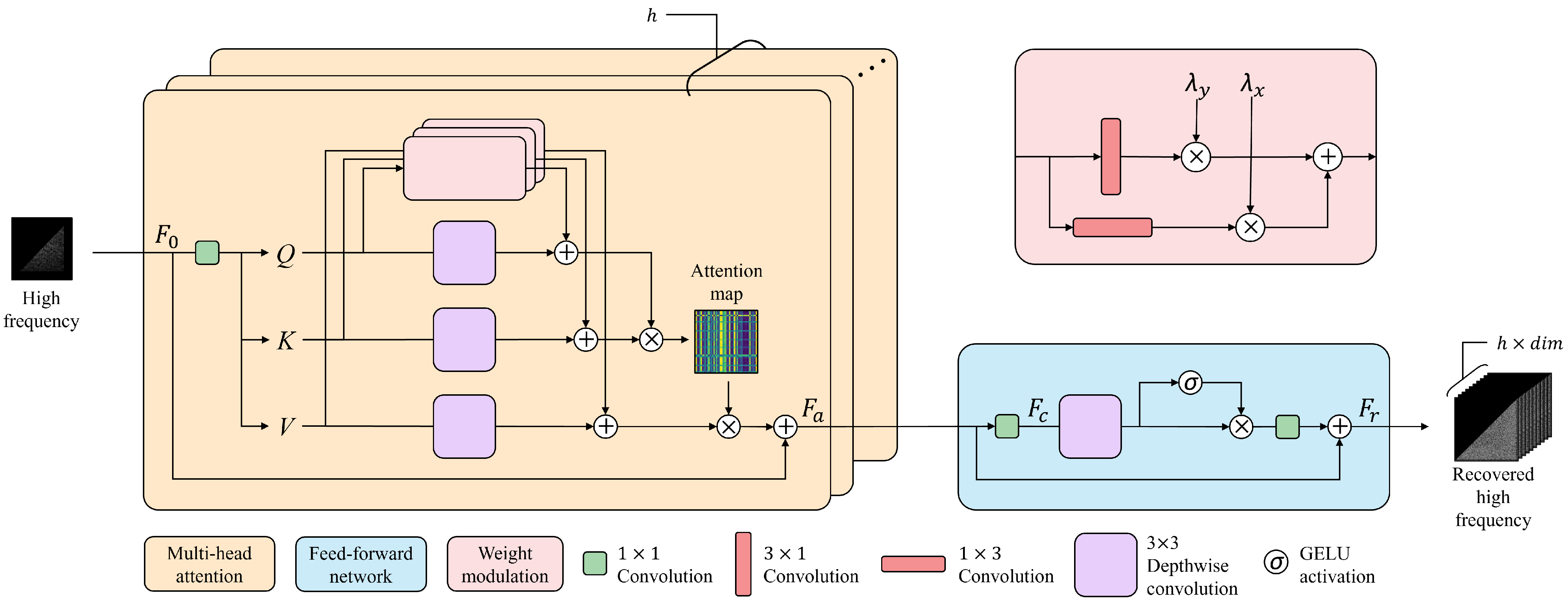
Figure 2.
Architecture of the m-DCTformer.
Figure 2.
Architecture of the m-DCTformer.
Figure 3.
Architecture of weight modulation transformer.
Figure 3.
Architecture of weight modulation transformer.
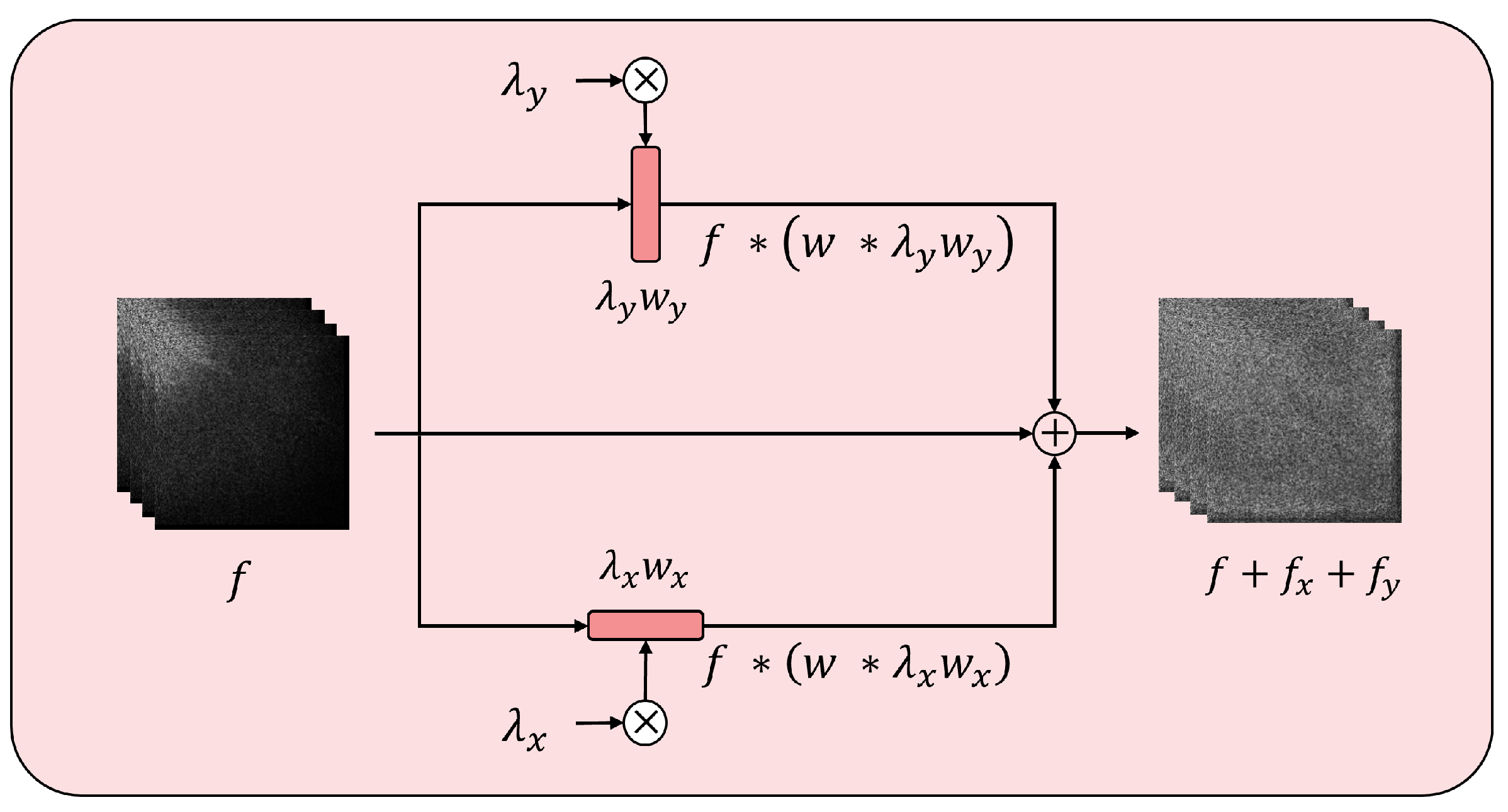
Figure 4.
Weight modulation process.
Figure 4.
Weight modulation process.
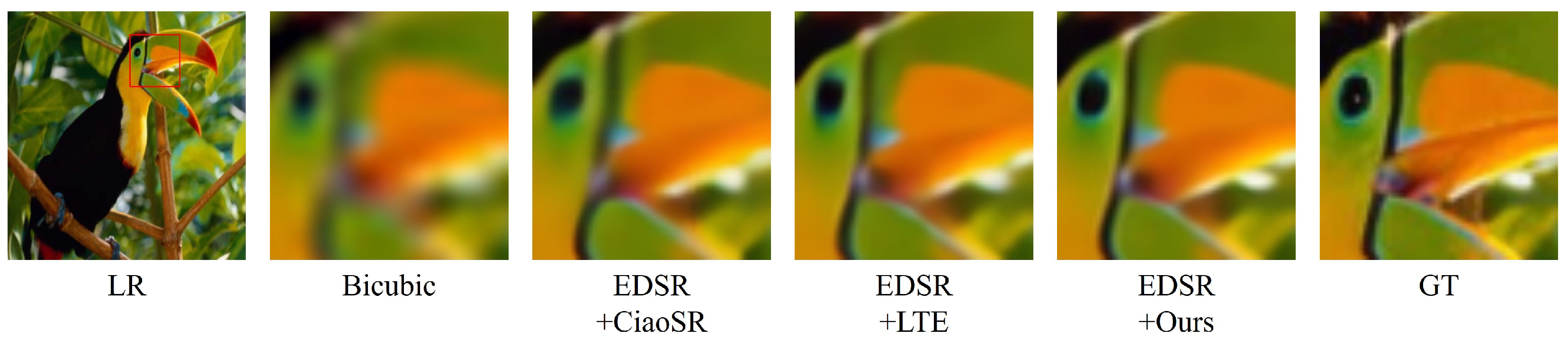
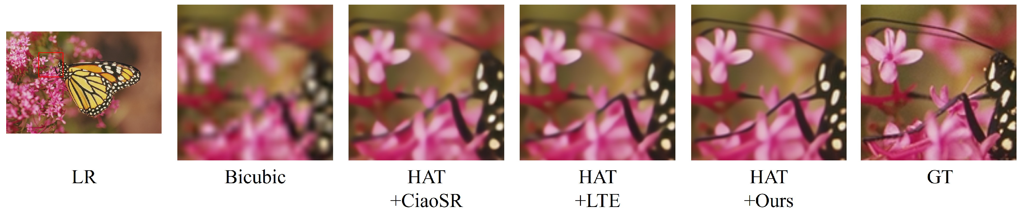
Figure 5.
Qualitative comparison of the m-DCTformer with other arbitrary scale super-resolution methods for a scale factor of ×4.9 on the Set5 dataset.
Figure 5.
Qualitative comparison of the m-DCTformer with other arbitrary scale super-resolution methods for a scale factor of ×4.9 on the Set5 dataset.
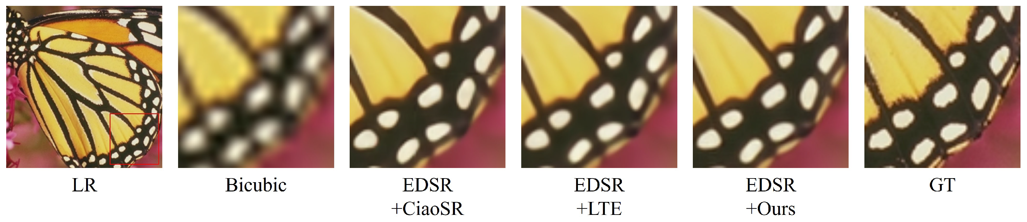
Figure 6.
Qualitative comparison of the m-DCTformer with other arbitrary scale super-resolution methods for a scale factor of ×4.9 on the Set5 dataset.
Figure 6.
Qualitative comparison of the m-DCTformer with other arbitrary scale super-resolution methods for a scale factor of ×4.9 on the Set5 dataset.
Figure 7.
Qualitative comparison of the m-DCTformer with other arbitrary-scale super-resolution methods for a scale factor of ×4.9 on the Set 14 dataset.
Figure 7.
Qualitative comparison of the m-DCTformer with other arbitrary-scale super-resolution methods for a scale factor of ×4.9 on the Set 14 dataset.
Figure 8.
Qualitative comparison of the m-DCTformer with other arbitrary scale super-resolution methods for a scale factor of ×4.9 on the Set 14 dataset.
Figure 8.
Qualitative comparison of the m-DCTformer with other arbitrary scale super-resolution methods for a scale factor of ×4.9 on the Set 14 dataset.
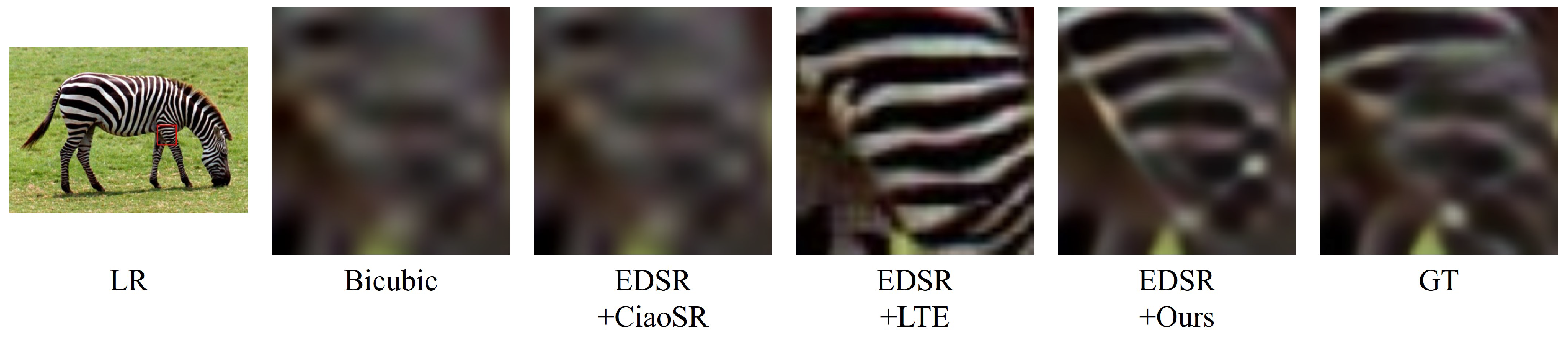
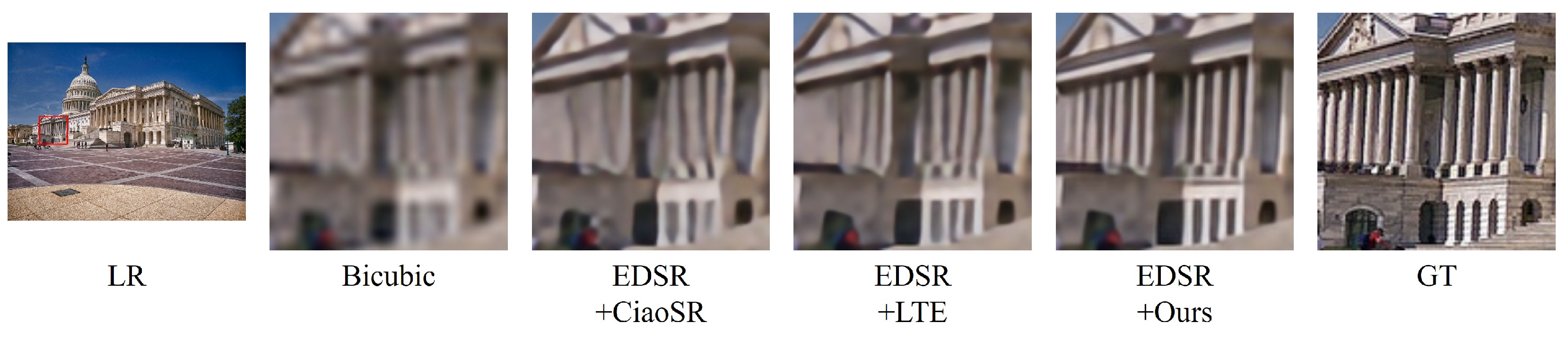
Figure 9.
Qualitative comparison of the m-DCTformer with other arbitrary scale super-resolution methods for a scale factor of ×4.9 on the Urban 100 dataset.
Figure 9.
Qualitative comparison of the m-DCTformer with other arbitrary scale super-resolution methods for a scale factor of ×4.9 on the Urban 100 dataset.
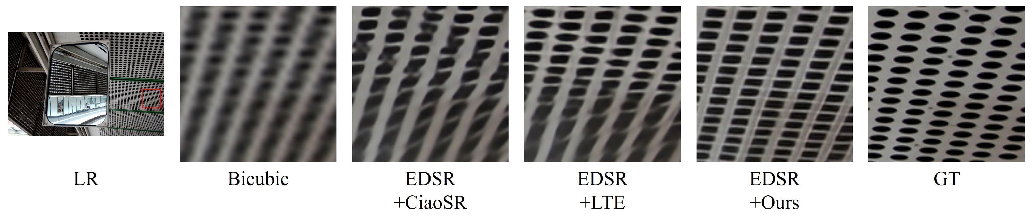
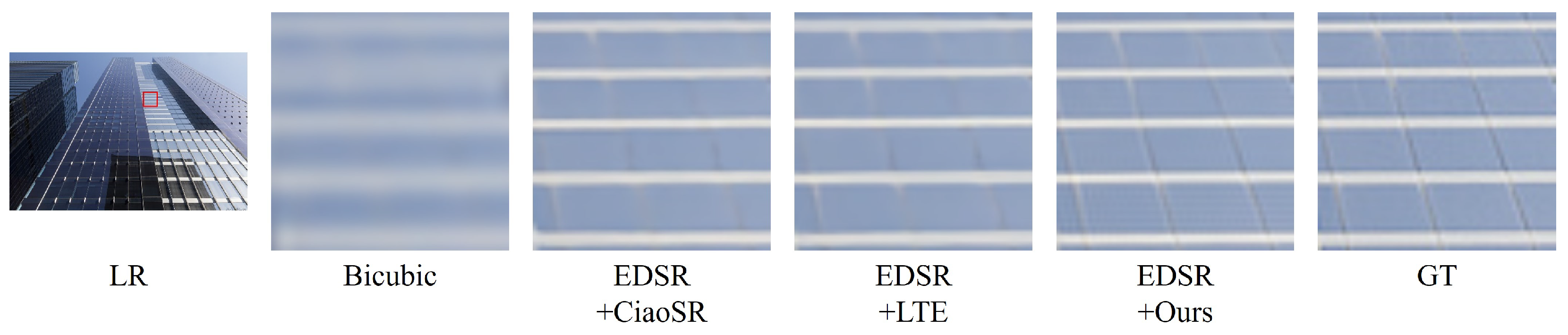
Figure 10.
Qualitative comparison of the m-DCTformer with other arbitrary scale super-resolution methods for a scale factor of ×4.9 on the Urban 100 dataset.
Figure 10.
Qualitative comparison of the m-DCTformer with other arbitrary scale super-resolution methods for a scale factor of ×4.9 on the Urban 100 dataset.
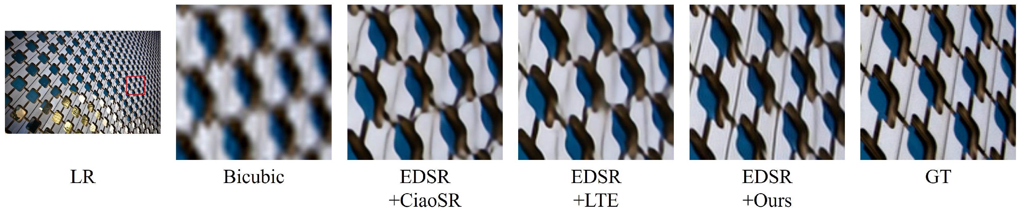
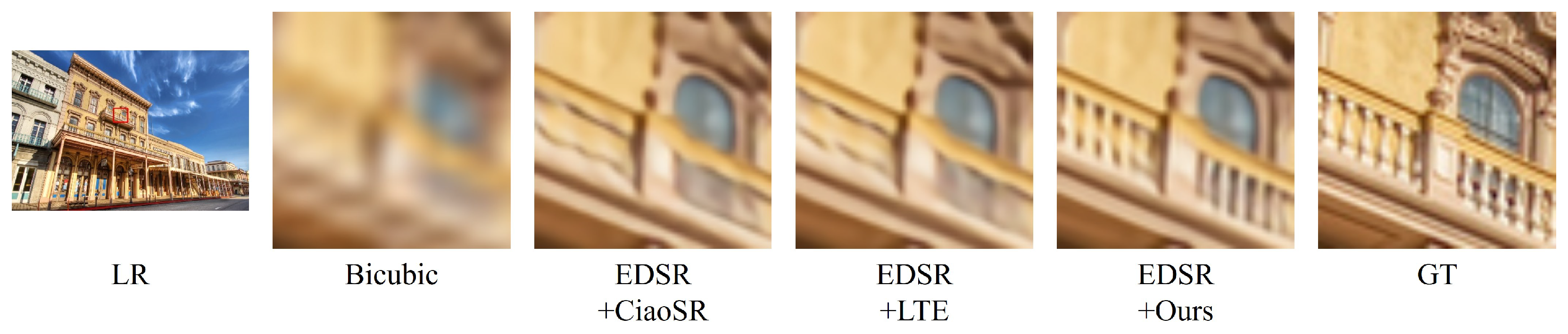
Figure 11.
Qualitative comparison of the m-DCTformer with other arbitrary scale super-resolution methods for a scale factor of ×4.9 on the Urban 100 dataset.
Figure 11.
Qualitative comparison of the m-DCTformer with other arbitrary scale super-resolution methods for a scale factor of ×4.9 on the Urban 100 dataset.
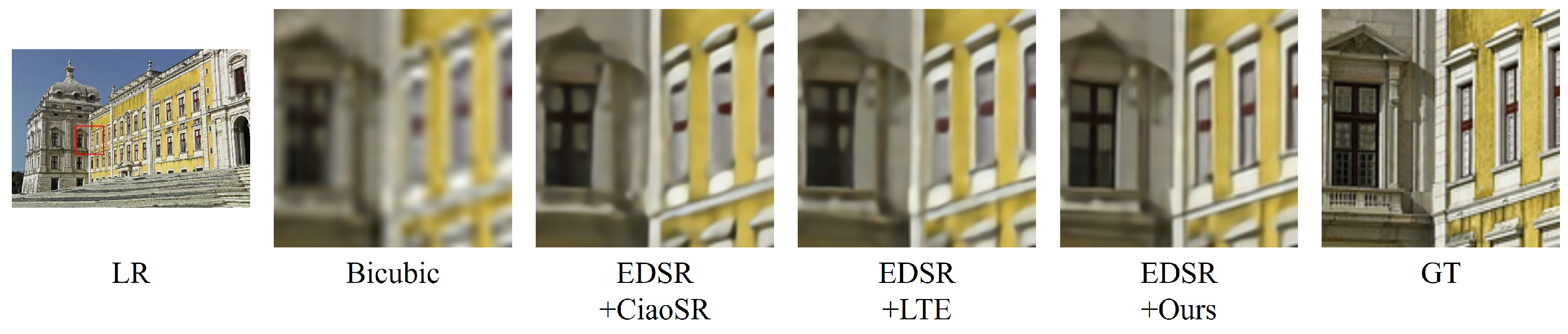
Figure 12.
Qualitative comparison of the m-DCTformer with other arbitrary scale super-resolution methods for a scale factor of ×4.9 on the Urban 100 dataset.
Figure 12.
Qualitative comparison of the m-DCTformer with other arbitrary scale super-resolution methods for a scale factor of ×4.9 on the Urban 100 dataset.
Figure 13.
Qualitative comparison of the m-DCTformer with other arbitrary scale super-resolution methods for a scale factor of ×3.1 on the Urban 100 dataset.
Figure 13.
Qualitative comparison of the m-DCTformer with other arbitrary scale super-resolution methods for a scale factor of ×3.1 on the Urban 100 dataset.
Figure 14.
Qualitative comparison of the m-DCTformer with other arbitrary scale super-resolution methods for a scale factor of ×3.1 on the Urban 100 dataset.
Figure 14.
Qualitative comparison of the m-DCTformer with other arbitrary scale super-resolution methods for a scale factor of ×3.1 on the Urban 100 dataset.
Figure 15.
Qualitative comparison of the m-DCTformer with other arbitrary-scale super-resolution methods for a scale factor of ×4.9 on the Set 14 dataset.
Figure 15.
Qualitative comparison of the m-DCTformer with other arbitrary-scale super-resolution methods for a scale factor of ×4.9 on the Set 14 dataset.
Figure 16.
Qualitative comparison of the m-DCTformer with other arbitrary scale super-resolution methods for a scale factor of ×4.9 on the Urban 100 dataset.
Figure 16.
Qualitative comparison of the m-DCTformer with other arbitrary scale super-resolution methods for a scale factor of ×4.9 on the Urban 100 dataset.
Figure 17.
Qualitative comparison of m-DCTformer with other arbitrary-scale super-resolution methods for a scale factor (×4.9) on the Urban 100 datasets.
Figure 17.
Qualitative comparison of m-DCTformer with other arbitrary-scale super-resolution methods for a scale factor (×4.9) on the Urban 100 datasets.
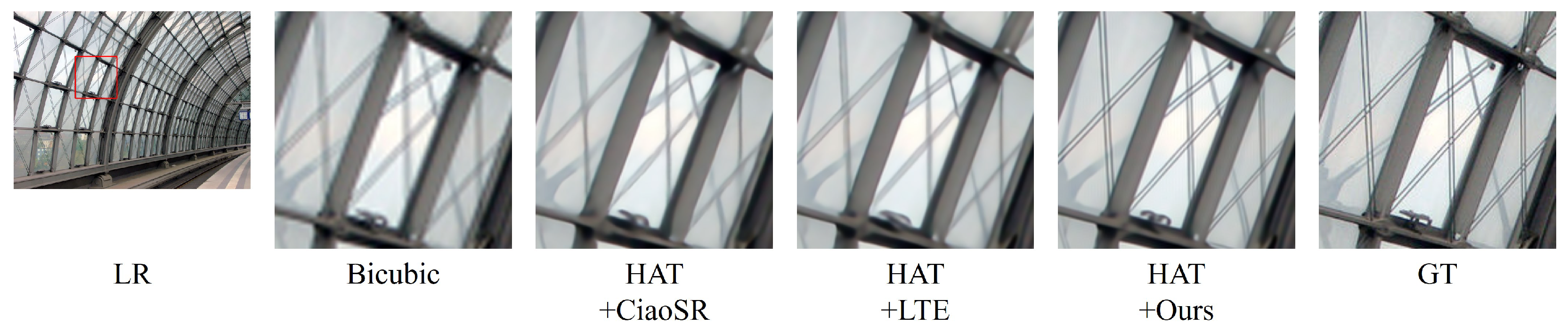
Figure 18.
Qualitative comparison of the m-DCTformer with other arbitrary scale super-resolution methods for a scale factor of ×2.9 on the real-world dataset.
Figure 18.
Qualitative comparison of the m-DCTformer with other arbitrary scale super-resolution methods for a scale factor of ×2.9 on the real-world dataset.
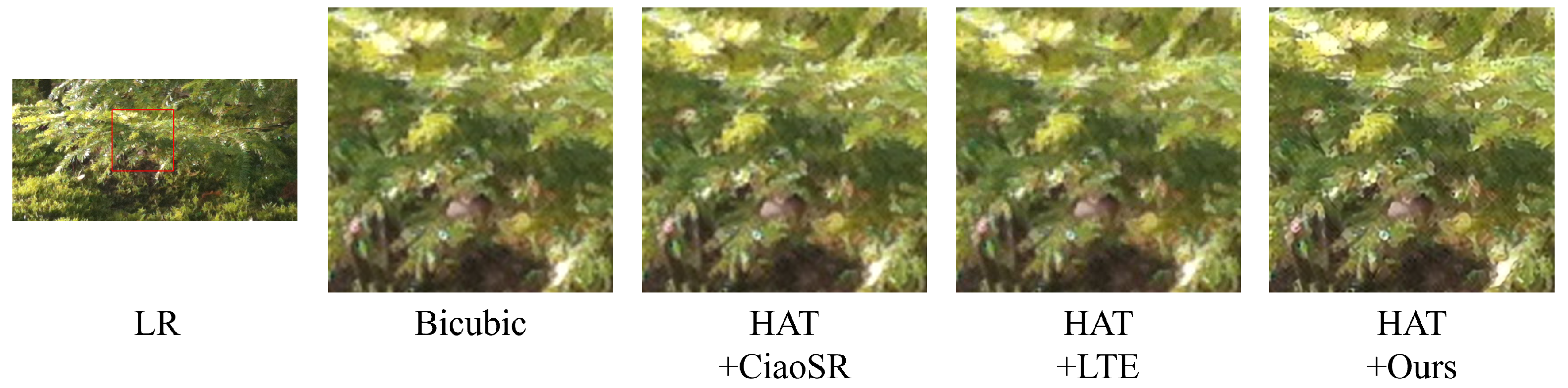
Figure 19.
Qualitative comparison of the m-DCTformer with other arbitrary scale super-resolution methods for a scale factor of ×2.9 on the real-world dataset.
Figure 19.
Qualitative comparison of the m-DCTformer with other arbitrary scale super-resolution methods for a scale factor of ×2.9 on the real-world dataset.
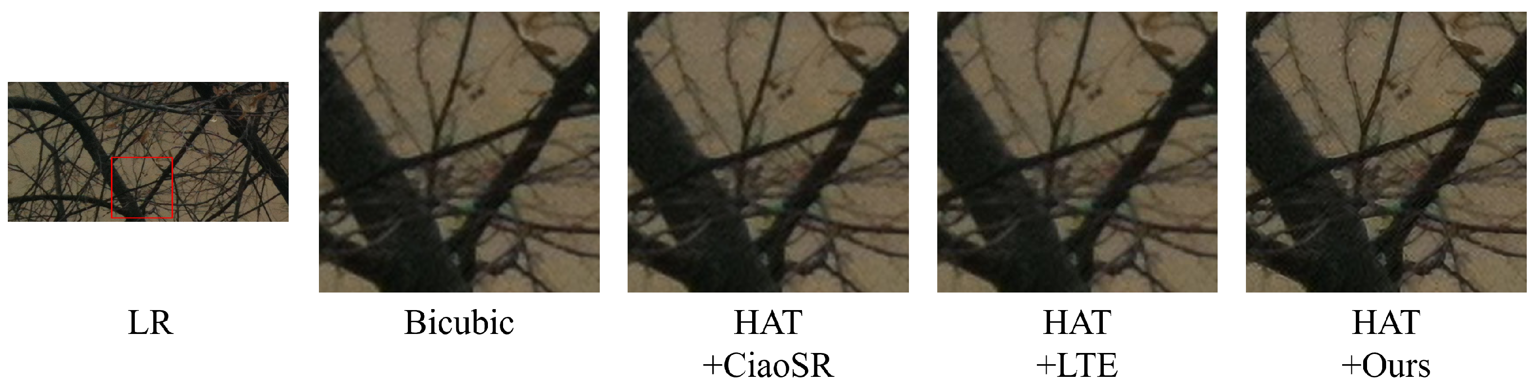
Figure 20.
Qualitative comparison of the m-DCTformer with other arbitrary scale super-resolution methods for a scale factor of ×2.9 on the real-world dataset.
Figure 20.
Qualitative comparison of the m-DCTformer with other arbitrary scale super-resolution methods for a scale factor of ×2.9 on the real-world dataset.
Table 1.
Quantitative results with other approaches and our m-DCTformer with EDSR and HAT on Set5 datasets. Bold represents the best peak signal-to-nose ratio (PSNR) and similarity index measure (SSIM) scores.
Table 1.
Quantitative results with other approaches and our m-DCTformer with EDSR and HAT on Set5 datasets. Bold represents the best peak signal-to-nose ratio (PSNR) and similarity index measure (SSIM) scores.
| Dataset | Set5 |
|---|
| Method | EDSR [19] + CiaoSR [5] | EDSR [19] + LTE [28] | EDSR [19] + ours |
| Metric | PSNR | SSIM | PSNR | SSIM | PSNR | SSIM |
| 2.1 | 37.35 | 0.9313 | 37.47 | 0.9559 | 37.51 | 0.9563 |
| 2.2 | 36.88 | 0.9265 | 37.05 | 0.9527 | 37.12 | 0.9533 |
| 2.3 | 36.58 | 0.9220 | 36.69 | 0.9494 | 36.77 | 0.9498 |
| 2.4 | 36.18 | 0.9176 | 36.30 | 0.9458 | 36.36 | 0.9462 |
| 2.5 | 35.86 | 0.9131 | 35.93 | 0.9425 | 35.99 | 0.9426 |
| 2.6 | 35.54 | 0.9086 | 35.65 | 0.9394 | 35.67 | 0.9393 |
| 2.7 | 35.23 | 0.9042 | 35.28 | 0.9362 | 35.31 | 0.9360 |
| 2.8 | 34.92 | 0.8996 | 34.97 | 0.9329 | 35.01 | 0.9326 |
| 2.9 | 34.60 | 0.8956 | 34.75 | 0.9298 | 34.74 | 0.9293 |
| 3.1 | 34.13 | 0.8871 | 34.19 | 0.9228 | 34.40 | 0.9257 |
| 3.2 | 33.92 | 0.8834 | 34.03 | 0.9200 | 34.22 | 0.9231 |
| 3.3 | 33.65 | 0.8786 | 33.76 | 0.9166 | 33.98 | 0.9201 |
| 3.4 | 33.45 | 0.8742 | 33.53 | 0.9131 | 33.72 | 0.9169 |
| 3.5 | 33.23 | 0.8708 | 33.30 | 0.9104 | 33.47 | 0.9138 |
| 3.6 | 32.95 | 0.8667 | 32.98 | 0.9054 | 33.12 | 0.9090 |
| 3.7 | 32.75 | 0.8628 | 32.73 | 0.9018 | 32.93 | 0.9064 |
| 3.8 | 32.53 | 0.5857 | 32.58 | 0.8989 | 32.73 | 0.9032 |
| 3.9 | 32.35 | 0.8546 | 32.37 | 0.8945 | 32.51 | 0.8993 |
| 4.1 | 31.99 | 0.8474 | 31.98 | 0.8875 | 32.17 | 0.8942 |
| 4.2 | 31.83 | 0.8440 | 31.84 | 0.8843 | 32.10 | 0.8914 |
| 4.3 | 31.62 | 0.8394 | 31.60 | 0.8801 | 31.85 | 0.8878 |
| 4.4 | 31.38 | 0.8356 | 31.43 | 0.8769 | 31.71 | 0.8853 |
| 4.5 | 31.24 | 0.8328 | 31.23 | 0.8722 | 31.56 | 0.8825 |
| 4.6 | 30.98 | 0.8279 | 31.08 | 0.8684 | 31.43 | 0.8797 |
| 4.7 | 30.85 | 0.8251 | 30.88 | 0.8645 | 31.21 | 0.8761 |
| 4.8 | 30.70 | 0.8221 | 30.75 | 0.8623 | 31.03 | 0.8733 |
| 4.9 | 30.53 | 0.8166 | 30.50 | 0.8565 | 30.84 | 0.8690 |
| Method | HAT [32] + CiaoSR [5] | HAT [32] + LTE [28] | HAT [32] + ours |
| Metric | PSNR | SSIM | PSNR | SSIM | PSNR | SSIM |
| 2.1 | 37.46 | 0.9522 | 37.67 | 0.9567 | 37.94 | 0.9587 |
| 2.2 | 36.97 | 0.9472 | 37.27 | 0.9537 | 37.52 | 0.9556 |
| 2.3 | 36.67 | 0.9429 | 36.90 | 0.9505 | 37.14 | 0.9522 |
| 2.4 | 36.24 | 0.9414 | 36.51 | 0.9471 | 36.71 | 0.9488 |
| 2.5 | 35.94 | 0.9401 | 36.17 | 0.9441 | 36.27 | 0.9452 |
| 2.6 | 35.60 | 0.9396 | 35.87 | 0.9409 | 35.96 | 0.9419 |
| 2.7 | 35.31 | 0.9351 | 35.51 | 0.9377 | 35.55 | 0.9382 |
| 2.8 | 35.00 | 0.9305 | 35.26 | 0.9348 | 35.24 | 0.9349 |
| 2.9 | 34.71 | 0.9268 | 35.00 | 0.9319 | 35.02 | 0.9319 |
| 3.1 | 34.22 | 0.9218 | 34.50 | 0.9255 | 35.00 | 0.9305 |
| 3.2 | 33.99 | 0.9200 | 34.32 | 0.9226 | 34.80 | 0.9278 |
| 3.3 | 33.72 | 0.9151 | 34.07 | 0.9197 | 34.52 | 0.9250 |
| 3.4 | 33.56 | 0.9119 | 33.86 | 0.9164 | 34.31 | 0.9226 |
| 3.5 | 33.30 | 0.9084 | 33.60 | 0.9132 | 34.13 | 0.9201 |
| 3.6 | 33.01 | 0.9059 | 33.25 | 0.9085 | 33.83 | 0.9162 |
| 3.7 | 32.80 | 0.9018 | 33.08 | 0.9055 | 33.57 | 0.9128 |
| 3.8 | 32.60 | 0.8984 | 32.89 | 0.9025 | 33.44 | 0.9101 |
| 3.9 | 32.39 | 0.8942 | 32.64 | 0.8975 | 33.13 | 0.9065 |
| 4.1 | 32.01 | 0.8899 | 32.28 | 0.8919 | 32.92 | 0.9032 |
| 4.2 | 31.87 | 0.8843 | 32.22 | 0.8889 | 32.78 | 0.9009 |
| 4.3 | 31.71 | 0.8807 | 32.00 | 0.8852 | 32.61 | 0.8977 |
| 4.4 | 31.50 | 0.8769 | 31.78 | 0.8812 | 32.50 | 0.8963 |
| 4.5 | 31.34 | 0.8726 | 31.62 | 0.8778 | 32.29 | 0.8929 |
| 4.6 | 31.10 | 0.8701 | 31.44 | 0.8739 | 32.11 | 0.8894 |
| 4.7 | 30.97 | 0.8676 | 31.28 | 0.8703 | 31.99 | 0.8873 |
| 4.8 | 30.79 | 0.8659 | 31.10 | 0.8680 | 31.73 | 0.8846 |
| 4.9 | 30.67 | 0.8601 | 30.90 | 0.8627 | 31.62 | 0.8819 |
Table 2.
Quantitative results with other approaches and our m-DCTformer with EDSR and HAT on Set14 datasets. Bold represents the best peak signal-to-nose ratio (PSNR) and similarity index measure (SSIM) scores.
Table 2.
Quantitative results with other approaches and our m-DCTformer with EDSR and HAT on Set14 datasets. Bold represents the best peak signal-to-nose ratio (PSNR) and similarity index measure (SSIM) scores.
| Dataset | Set14 |
|---|
| Method | EDSR [19] + CiaoSR [5] | EDSR [19] + LTE [28] | EDSR [19] + ours |
| Metric | PSNR | SSIM | PSNR | SSIM | PSNR | SSIM |
| 2.1 | 32.91 | 0.8801 | 33.19 | 0.9117 | 33.30 | 0.9123 |
| 2.2 | 32.52 | 0.8690 | 32.70 | 0.9029 | 32.83 | 0.9036 |
| 2.3 | 32.13 | 0.8594 | 32.31 | 0.8955 | 32.41 | 0.8960 |
| 2.4 | 31.81 | 0.8510 | 31.99 | 0.8888 | 32.08 | 0.8885 |
| 2.5 | 31.50 | 0.8418 | 31.63 | 0.8807 | 31.71 | 0.8803 |
| 2.6 | 31.19 | 0.8336 | 31.33 | 0.8727 | 31.40 | 0.8720 |
| 2.7 | 30.92 | 0.8252 | 31.05 | 0.8656 | 31.08 | 0.8645 |
| 2.8 | 30.73 | 0.8188 | 30.78 | 0.8583 | 30.79 | 0.8569 |
| 2.9 | 30.43 | 0.8093 | 30.50 | 0.8511 | 30.51 | 0.8495 |
| 3.1 | 30.13 | 0.7958 | 30.12 | 0.8374 | 30.25 | 0.8387 |
| 3.2 | 29.88 | 0.7878 | 29.94 | 0.8310 | 30.02 | 0.8323 |
| 3.3 | 29.70 | 0.7811 | 29.73 | 0.8239 | 29.83 | 0.8258 |
| 3.4 | 29.53 | 0.7742 | 29.54 | 0.8173 | 29.65 | 0.8196 |
| 3.5 | 29.37 | 0.7678 | 29.39 | 0.8110 | 29.49 | 0.8134 |
| 3.6 | 29.20 | 0.7614 | 29.24 | 0.8058 | 29.33 | 0.8085 |
| 3.7 | 29.05 | 0.7550 | 29.03 | 0.7988 | 29.10 | 0.8014 |
| 3.8 | 28.89 | 0.7497 | 28.86 | 0.7925 | 28.95 | 0.7956 |
| 3.9 | 28.75 | 0.7431 | 28.76 | 0.7879 | 28.83 | 0.7914 |
| 4.1 | 28.48 | 0.7309 | 28.48 | 0.7755 | 28.61 | 0.7816 |
| 4.2 | 28.35 | 0.7259 | 28.36 | 0.7701 | 28.51 | 0.7771 |
| 4.3 | 28.23 | 0.7209 | 28.19 | 0.7637 | 28.41 | 0.7720 |
| 4.4 | 28.10 | 0.7154 | 28.10 | 0.7583 | 28.29 | 0.7677 |
| 4.5 | 27.96 | 0.7105 | 27.95 | 0.7530 | 28.11 | 0.7621 |
| 4.6 | 27.84 | 0.7052 | 27.81 | 0.7474 | 27.93 | 0.7570 |
| 4.7 | 27.73 | 0.6998 | 27.72 | 0.7426 | 27.85 | 0.7529 |
| 4.8 | 27.60 | 0.6944 | 27.62 | 0.7377 | 27.71 | 0.7480 |
| 4.9 | 27.49 | 0.6910 | 27.46 | 0.7309 | 27.59 | 0.7424 |
| Method | HAT [32] + CiaoSR [5] | HAT [32] + LTE [28] | HAT [32] + ours |
| Metric | PSNR | SSIM | PSNR | SSIM | PSNR | SSIM |
| 2.1 | 33.73 | 0.9179 | 33.57 | 0.9148 | 34.16 | 0.9200 |
| 2.2 | 33.27 | 0.9108 | 33.01 | 0.9064 | 33.62 | 0.9114 |
| 2.3 | 32.90 | 0.9014 | 32.64 | 0.8995 | 33.21 | 0.9044 |
| 2.4 | 32.56 | 0.8956 | 32.30 | 0.8925 | 32.81 | 0.8975 |
| 2.5 | 32.22 | 0.8873 | 31.88 | 0.8839 | 32.41 | 0.8894 |
| 2.6 | 31.89 | 0.8808 | 31.58 | 0.8760 | 32.03 | 0.8812 |
| 2.7 | 31.61 | 0.8729 | 31.26 | 0.8689 | 31.66 | 0.8732 |
| 2.8 | 31.31 | 0.8643 | 30.99 | 0.8619 | 31.34 | 0.8655 |
| 2.9 | 31.03 | 0.8576 | 30.72 | 0.8551 | 31.04 | 0.8577 |
| 3.1 | 30.95 | 0.8490 | 30.30 | 0.8415 | 31.01 | 0.8496 |
| 3.2 | 30.38 | 0.8409 | 30.11 | 0.8353 | 30.74 | 0.8437 |
| 3.3 | 30.22 | 0.8335 | 29.91 | 0.8283 | 30.52 | 0.8368 |
| 3.4 | 30.03 | 0.8282 | 29.75 | 0.8220 | 30.29 | 0.8304 |
| 3.5 | 29.84 | 0.8200 | 29.58 | 0.8157 | 30.11 | 0.8243 |
| 3.6 | 29.68 | 0.8156 | 29.41 | 0.8104 | 29.94 | 0.8197 |
| 3.7 | 29.69 | 0.8088 | 29.21 | 0.8031 | 29.69 | 0.8134 |
| 3.8 | 29.35 | 0.8042 | 29.03 | 0.7973 | 29.52 | 0.8074 |
| 3.9 | 29.20 | 0.7998 | 28.95 | 0.7929 | 29.41 | 0.8030 |
| 4.1 | 28.88 | 0.7901 | 28.70 | 0.7816 | 29.14 | 0.7941 |
| 4.2 | 28.73 | 0.7825 | 28.59 | 0.7761 | 29.02 | 0.7888 |
| 4.3 | 28.63 | 0.7780 | 28.45 | 0.7702 | 28.87 | 0.7836 |
| 4.4 | 28.47 | 0.7725 | 28.37 | 0.7656 | 28.81 | 0.7798 |
| 4.5 | 28.33 | 0.7704 | 28.11 | 0.7588 | 28.67 | 0.7748 |
| 4.6 | 28.22 | 0.7638 | 27.94 | 0.7534 | 28.51 | 0.7710 |
| 4.7 | 28.09 | 0.7595 | 27.86 | 0.7488 | 28.42 | 0.7666 |
| 4.8 | 27.96 | 0.7438 | 27.76 | 0.7437 | 28.28 | 0.7624 |
| 4.9 | 27.83 | 0.7401 | 27.71 | 0.7386 | 28.17 | 0.7571 |
Table 3.
Quantitative results with other approaches and our m-DCTformer with EDSR and HAT on Urban100 datasets. Bold represents the best peak signal-to-nose ratio (PSNR) and similarity index measure (SSIM) scores.
Table 3.
Quantitative results with other approaches and our m-DCTformer with EDSR and HAT on Urban100 datasets. Bold represents the best peak signal-to-nose ratio (PSNR) and similarity index measure (SSIM) scores.
| Dataset | Urban100 |
|---|
| Method | EDSR [19] + CiaoSR [5] | EDSR [19] + LTE [28] | EDSR [19] + ours |
| Metric | PSNR | SSIM | PSNR | SSIM | PSNR | SSIM |
| 2.1 | 30.85 | 0.9196 | 31.70 | 0.9224 | 32.00 | 0.9246 |
| 2.2 | 30.25 | 0.9105 | 31.20 | 0.9150 | 31.42 | 0.9166 |
| 2.3 | 29.65 | 0.9002 | 30.74 | 0.9076 | 30.87 | 0.9082 |
| 2.4 | 29.32 | 0.8948 | 30.33 | 0.9004 | 30.37 | 0.8999 |
| 2.5 | 28.95 | 0.8873 | 29.92 | 0.8929 | 29.91 | 0.8917 |
| 2.6 | 28.65 | 0.8798 | 29.56 | 0.8856 | 29.47 | 0.8831 |
| 2.7 | 28.14 | 0.8649 | 29.21 | 0.8783 | 29.07 | 0.8750 |
| 2.8 | 28.06 | 0.8665 | 28.89 | 0.8712 | 28.70 | 0.8667 |
| 2.9 | 27.87 | 0.8601 | 28.60 | 0.8643 | 28.38 | 0.8588 |
| 3.1 | 27.16 | 0.8460 | 28.07 | 0.8507 | 28.46 | 0.8573 |
| 3.2 | 26.94 | 0.8380 | 27.83 | 0.8441 | 28.20 | 0.8508 |
| 3.3 | 26.66 | 0.8318 | 27.60 | 0.8372 | 27.93 | 0.8437 |
| 3.4 | 26.47 | 0.8242 | 27.38 | 0.8307 | 27.69 | 0.8372 |
| 3.5 | 26.24 | 0.8176 | 27.16 | 0.8239 | 27.46 | 0.8304 |
| 3.6 | 26.09 | 0.8120 | 26.96 | 0.8173 | 27.24 | 0.8239 |
| 3.7 | 25.88 | 0.8041 | 26.76 | 0.8107 | 27.03 | 0.8172 |
| 3.8 | 25.72 | 0.7990 | 26.58 | 0.8044 | 26.82 | 0.8109 |
| 3.9 | 25.55 | 0.7930 | 26.41 | 0.7981 | 26.64 | 0.8046 |
| 4.1 | 25.22 | 0.7806 | 26.07 | 0.7851 | 26.43 | 0.7964 |
| 4.2 | 25.07 | 0.7741 | 25.91 | 0.7788 | 26.27 | 0.7907 |
| 4.3 | 24.94 | 0.7686 | 25.77 | 0.7731 | 26.12 | 0.7853 |
| 4.4 | 24.78 | 0.7643 | 25.62 | 0.7666 | 25.97 | 0.7795 |
| 4.5 | 24.49 | 0.7494 | 25.49 | 0.7610 | 25.84 | 0.7744 |
| 4.6 | 24.57 | 0.7550 | 25.34 | 0.7544 | 25.69 | 0.7685 |
| 4.7 | 24.26 | 0.7401 | 25.21 | 0.7487 | 25.55 | 0.7629 |
| 4.8 | 30.70 | 0.8221 | 25.09 | 0.7431 | 25.42 | 0.7579 |
| 4.9 | 30.53 | 0.8166 | 24.96 | 0.7369 | 25.28 | 0.7522 |
| Method | HAT [32] + CiaoSR [5] | HAT [32] + LTE [28] | HAT [32] + ours |
| Metric | PSNR | SSIM | PSNR | SSIM | PSNR | SSIM |
| 2.1 | 32.66 | 0.9302 | 32.45 | 0.9295 | 33.32 | 0.9373 |
| 2.2 | 32.10 | 0.9253 | 31.93 | 0.9227 | 32.63 | 0.9302 |
| 2.3 | 31.38 | 0.9138 | 31.47 | 0.9159 | 32.00 | 0.9227 |
| 2.4 | 31.10 | 0.9101 | 31.03 | 0.9092 | 31.45 | 0.9150 |
| 2.5 | 30.71 | 0.9036 | 30.63 | 0.9025 | 30.92 | 0.9072 |
| 2.6 | 30.35 | 0.8977 | 30.24 | 0.8956 | 30.43 | 0.8992 |
| 2.7 | 29.46 | 0.8842 | 29.89 | 0.8890 | 29.98 | 0.8913 |
| 2.8 | 29.73 | 0.8857 | 29.56 | 0.8822 | 29.57 | 0.8834 |
| 2.9 | 29.45 | 0.8794 | 29.27 | 0.8759 | 29.19 | 0.8756 |
| 3.1 | 28.98 | 0.8758 | 28.70 | 0.8731 | 30.26 | 0.8876 |
| 3.2 | 28.81 | 0.8701 | 28.46 | 0.877 | 29.94 | 0.8821 |
| 3.3 | 28.65 | 0.8728 | 28.22 | 0.8704 | 29.61 | 0.8758 |
| 3.4 | 28.51 | 0.8692 | 27.98 | 0.8643 | 29.32 | 0.8699 |
| 3.5 | 28.18 | 0.8601 | 27.76 | 0.8581 | 29.02 | 0.8638 |
| 3.6 | 27.96 | 0.8552 | 27.55 | 0.8520 | 28.75 | 0.8578 |
| 3.7 | 27.79 | 0.8497 | 27.36 | 0.8459 | 28.49 | 0.8519 |
| 3.8 | 27.53 | 0.8424 | 27.17 | 0.8400 | 28.27 | 0.8463 |
| 3.9 | 27.41 | 0.8374 | 26.99 | 0.8339 | 28.04 | 0.8405 |
| 4.1 | 27.23 | 0.8367 | 26.62 | 0.8319 | 28.18 | 0.8404 |
| 4.2 | 26.92 | 0.8290 | 26.46 | 0.8259 | 27.98 | 0.8354 |
| 4.3 | 26.75 | 0.8242 | 26.32 | 0.8205 | 27.82 | 0.8311 |
| 4.4 | 26.65 | 0.8191 | 26.16 | 0.8144 | 27.63 | 0.8258 |
| 4.5 | 26.61 | 0.8153 | 26.03 | 0.8093 | 27.45 | 0.8211 |
| 4.6 | 26.31 | 0.8102 | 25.88 | 0.8033 | 27.30 | 0.8163 |
| 4.7 | 26.12 | 0.8054 | 25.74 | 0.7976 | 27.13 | 0.8112 |
| 4.8 | 25.92 | 0.8007 | 25.62 | 0.7923 | 26.99 | 0.8071 |
| 4.9 | 25.71 | 0.7952 | 25.48 | 0.7864 | 26.84 | 0.8021 |
Table 4.
Comparison of the m-DCTformer with arbitrary-scale super-resolution approaches for FLOPs, parameters, model capacity, and time.
Table 4.
Comparison of the m-DCTformer with arbitrary-scale super-resolution approaches for FLOPs, parameters, model capacity, and time.
| | FLOPs (G) | Parameters (M) | Model Capacity (MB) | Time (ms) |
|---|
| EDSR [19] + CiaoSR [5] | 599 | 42.83 | 490 | 1340 |
| EDSR [19] + LTE [28] | 618 | 39.74 | 454 | 483 |
| EDSR [19] + ours | 538 | 47.75 | 155 | 391 |
Table 5.
Quantitative results with the m-DCTformer on the Set5 dataset for . Bold represents the best PSNR and SSIM scores.
Table 5.
Quantitative results with the m-DCTformer on the Set5 dataset for . Bold represents the best PSNR and SSIM scores.
| DCT Domain | Weight Modulation | PSNR | SSIM |
|---|
| | | 35.50 | 0.9335 |
| | 🗸 | 35.52 | 0.9335 |
| 🗸 | | 35.93 | 0.9424 |
| 🗸 | 🗸 | 35.99 | 0.9426 |
Table 6.
Quantitative results with the m-DCTformer on the Urban 100 dataset for . Bold represents the best PSNR and SSIM scores.
Table 6.
Quantitative results with the m-DCTformer on the Urban 100 dataset for . Bold represents the best PSNR and SSIM scores.
| DCT Domain | Weight Modulation | PSNR | SSIM |
|---|
| | | 29.58 | 0.8841 |
| | 🗸 | 29.61 | 0.8842 |
| 🗸 | | 29.84 | 0.8899 |
| 🗸 | 🗸 | 29.91 | 0.8917 |
Table 7.
Quantitative results with the m-DCTformer on the Set 14 dataset for . Bold represents the best PSNR and SSIM scores.
Table 7.
Quantitative results with the m-DCTformer on the Set 14 dataset for . Bold represents the best PSNR and SSIM scores.
| The Parameter d | Set14 |
|---|
| | PSNR | SSIM |
| 10 | 29.38 | 0.8128 |
| 20 | 29.49 | 0.8134 |
| 30 | 29.46 | 0.8133 |


