A Decoupling Method for Successive Robot Rotation Based on Time Domain Instantaneous Euler Angle

Abstract

In the present study, a novel time domain decoupling method was proposed for the multiple successive rotations of different kinds of robots. This is achieved through the utilization of instantaneous Euler angles. For a general parallel mechanism, the Plücker coordinates of the intersection line of the before and after rotation plane are determined through the reciprocal product principle of screw theory. Additionally, the angle between these two rotation planes is defined as the instantaneous Euler angle. The analysis of the general parallel mechanism was used as an example to illustrate the solution method of the instantaneous Euler angle. To investigate the intrinsic relationship between the instantaneous Euler angle and the conventional Euler angle, the mathematical mapping relationship and the difference between the instantaneous Euler angle and the two kinds of Euler angles (Z-Y-X and Z-Y-Z) were explored, respectively. Simulations of a 3-sps-s parallel mechanism and a robotic arm were employed to illustrate the superiority of the instantaneous Euler angle. The findings showed that the instantaneous Euler angle exhibited enhanced temporal consistency compared to the conventional Euler angle. Further, it is better suited for accurately describing the decoupled rotation of robotic systems. The proposed approach is also generally applicable to robot performance evaluation, mechanism design, and other relevant fields.

1. Introduction

The configuration design of existing robots is closely derived from bionic movements in nature. Most design methods equate the robot’s motion to several rotational joints or prismatic joints. However, bionic movement in nature is often irregular, so the corresponding equivalent rigid body movement is difficult to describe accurately [1,2]. In order to analyze the kinematic performance of a spatially rigid body, it is necessary to find a suitable description method that can accurately and clearly express the rotation performance. In addition, since different pose description methods are intrinsically linked, finding this intrinsic link can help in the selection of a suitable description method [3]. However, the existing literature [4,5,6,7,8] lacks in-depth studies on the description method of successive multiple rotations and the description methods of the intrinsic connections of the rigid body’s motion. Therefore, it is worthwhile to introduce a novel method to describe the decoupled rotation of the successive rotation and establish the intrinsic connection between different description methods with universal applicability.

It is well known that after the rotation of a rigid body, the components along different axes need to be further analyzed and evaluated [9,10,11,12]. The direction cosine matrices and homogeneous coordinate matrices are widely used to describe the rigid body motion [13,14]. The directional cosine matrix represents the directional cosine of three orthonormal vectors in a fixed coordinate system, i.e., R = [n o k], where R is an orthogonal matrix, six of the nine variables are restrained, and the other three variables are independent. Furthermore, after several successive rotations, the position of each axis is changed at least one time. Therefore, the direction and position of the axis should be obtained by summing the components of each direction vector. Currently, there are various mathematical expressions describing the motion of a rigid body, such as the Euler angle [15,16,17], the RPY angle [18], the Euler–Rodrigues parameter [19], and quaternion [20,21]. However, there is a common problem with these methods of describing the rotation of rigid bodies: the variables involved appear in different time domains, and time domain consistency is difficult to guarantee.

In the existing literature, the relationship between the orientation and position of robots after multiple successive rotations and the reference coordinate system is commonly presented, but the coupling angle of the axis after multiple successive rotations is not described, which has an important influence on the different fields that require accurate mathematical description [22,23,24,25,26]. In addition, the coupling angle helps to reveal the intrinsic connection between different posture description methods and provides a theoretic basis for selecting a suitable method to describe the motion of robots. Zhang et al. [27] analyzed the relationship between the normal motion of a moving platform and the intersection line of two rotation planes and obtained an expression for the coupling angle around the normal motion and its analytic expression. Huang et al. [28] represented the ridge line as the intersection line of the before and after rotation plane, and introduced a method to describe spatial motion using the Euler angle. Qu et al. [29] proposed a criterion for defining decoupled motion based on screw theory, and established conditions and implementation methods for the decoupled motion.

The analyses in the existing literature are mainly based on traditional methods of describing the rotations of robots, but the problem of the time domain consistency between multiple successive rotations remains to be solved. For example, the Z-Y-X Euler angles are used to illustrate the description of spatially rigid rotation (see Figure 1). If the target motion $\kappa \left(t\right)$ is expressed as a function of time, the x₀, y₀, and z₀ axes of the local coordinate system coincide with the x, y, and z axes of the global coordinate system prior to the rotation. The first rotation is rotated $\alpha$ around the z₀ axis by $\alpha$ degrees, and then the new coordinate system is defined as o-x₁y₁z₁, the interval time is expressed as interval $\Delta t_{01}$, and the instantaneous moment is expressed as $t_{01}$; the second rotation is rotated $\beta$ around the y₁ axis by $\beta$ degrees, the new coordinate system is defined as o-x₂y₂z₂, the interval time is expressed as $\Delta t_{02}$, and the instantaneous moment is expressed as $t_{02}$; the last rotation is rotated $\gamma$ around the x₂ axis by $\gamma$ degrees, the new coordinate system is defined as o-x₃y₃z₃, the interval time is expressed as $\Delta t_{03}$, and the instantaneous moment is expressed as $t_{03}$. Clearly, the corresponding rotations involve three rotation angles for each plane of rotation. Usually, the rotation performance of robots is represented by the Euler angles $\alpha$, $\beta$, and $\gamma$. However, from the initial rotation state $\kappa \left(t_0\right)$ to the final motion state $\kappa \left(t_3\right)$, these three angles appear in different time domains, and the internal relationships vary from time to time, which is called time domain inconsistency. That is, for multiple successive rotations of a robot, it is not appropriate to use the conventional Euler angle to describe the instantaneous rotation at a particular moment.

$$\kappa \left(t_0\right)\stackrel{\alpha \left(t_{01}\right)\to \beta \left(t_{02}\right)\to \gamma \left(t_{03}\right)}{\to }\kappa \left(t_1\right)$$

(1)

where $\begin{array}{l}{t}_{01}=t_0+\Delta t_{01}\\ t_{02}=t_1+\Delta t_{01}+\Delta t_{02}\\ t_{03}=t_1+\Delta t_{01}+\Delta t_{02}+\Delta t_{03}\end{array}$.

In order to solve the problem of the time domain inconsistency, this paper decouples the traditional Euler angles into three rotation directions, and establishes the inner relationship between the decoupled rotation angle and the Euler angle. The structure of this article is as follows: Section 2 introduces the basic principle of the mathematical method used in this paper. In Section 3, a general parallel mechanism is set as an example, and we introduce the deriving process of the instantaneous Euler angle. In Section 4, we discuss the intrinsic relationship between the instantaneous Euler angle and different forms of the conventional Euler angles. In Section 5, in order to illustrate the application of the instantaneous Euler angle, we choose a 3-sps-s parallel mechanism and a robotic arm to investigate the description of the robots’ motion performance. Lastly, the conclusion of this paper is presented.

2. Introduction of the Basic Principles of Euler Angle Decoupling

2.1. Introduction of the Conventional Euler Angle

A common method to describe the rotation of robots is the Z-Y-X Euler angle [2,3]. Initially, the x₀ axis, y₀ axis, and z₀ axis of the local coordinate system coincide with the x, y, and z axes of the global coordinate system. The first rotation rotates by $\alpha$ degrees around the z₀ axis, and the new coordinate system is defined as o-x₁y₁z₁; the second rotation rotates by $\beta$ degrees around the y₁ axis, and the new coordinate system is defined as x₂y₂z₂; the last rotation rotates $\gamma$ degrees around the x₂ axis, and the new coordinate system is defined as o-x₃y₃z₃. This process is called the Z-Y-X rotation type, where the three rotations vary around different axes. In the existing literature, the description of rigid body motion and the decoupling motion of robots are mainly analyzed according to the conventional Euler angle. For instance, the authors in [30] propose a kinematic hybrid decoupling parallel mechanism based on the geometry method. Li et al. [31] analyze the degree of freedom of the coupling mechanism with the help of the cell differentiation principle. In [32], a three-DOF decoupled parallel mechanism is proposed using the combination of different kinds of joints. However, the description of these decoupling mechanisms adopts the conventional Euler angle, without considering the continuity of the robot in the time domain.

Usually, the conventional Euler angles represent the rotation along a specified linear vector axis or bivector axis, i.e., the rotational motion or transitional motion of a rigid body along the x, y, or z axis of a local coordinate system. The ridges represent the intersection lines before and after the plane of rotation [28]. Finding the ridge line is helpful to achieve an objective method of measuring the direction and magnitude of the spatial rotation [33]. Therefore, determining the ridge line and calculating the Euler angles are very important for analyzing the rotation of the parallel mechanism. Generally, the conventional ridge line of a single rigid body appears at the completion of the second rotation, and the third rotation does not affect the position of the ridge lines; however, the rotation of a robot is always carried out along three directions, and the rotation directions interact with each other. Therefore, in this paper, the ridge line is represented as three axes along different directions, which are the intersection lines of the before and after rotation planes in the XY plane, the YZ plane, and the XZ plane, respectively; then, the corresponding rotation angles are represented as the instantaneous Euler angles.

2.2. Introduction of Reciprocal Product Principle

As mentioned before, the instantaneous Euler angle represents the intersection line of the before and after rotation plane, including the scalar value of the instantaneous Euler angle and the position and direction of the ridge line. When solving the ridge line, the corresponding instantaneous Euler angle can also be solved. In this paper, the principle of the reciprocal product of the screw theory is introduced to solve the above problem. Firstly, the three line vectors are expressed as below:

$$\begin{array}{l}{\mathsf{\$}}_1=\left(S_1;S_{01}\right)=(\begin{array}{ccc}{l}_1& m_1& n_1\end{array};\begin{array}{ccc}{O}_1& P_1& Q_1\end{array})\\ {\mathsf{\$}}_2=\left(S_2;S_{02}\right)=(\begin{array}{ccc}{l}_2& m_2& n_2\end{array};\begin{array}{ccc}{O}_2& P_2& Q_2\end{array})\\ {\mathsf{\$}}_3=\left(S_3;S_{03}\right)=(\begin{array}{ccc}{l}_3& m_3& n_3\end{array};\begin{array}{ccc}{O}_3& P_3& Q_3\end{array})\end{array}$$

(2)

By definition, if there exists a ridge line with intersection lines that do not intersect with the other three lines, the screw of the ridge line must be reciprocal to the other three-line vectors. If the ridge line is expressed as ${\mathsf{\$}}_r=\left(S;S_0\right)=(\begin{array}{ccc}l& m& n\end{array};\begin{array}{ccc}O& P& Q\end{array})$, the algebraic equations can be obtained according to the principle of the reciprocal product of the screw theory:

$$\begin{array}{l}l{O}_1+m{P}_1+n{Q}_1+l_{1}O+m_{1}P+n_{1}Q=0\\ l{O}_2+m{P}_2+n{Q}_2+l_{2}O+m_{2}P+n_{2}Q=0\\ l{O}_3+m{P}_3+n{Q}_3+l_{3}O+m_{3}P+n_{3}Q=0\end{array}$$

(3)

However, the number of unknown variables is greater than the number of algebraic equations, i.e., there are infinite such solutions satisfying the condition. In addition, three of the basic solution systems are linearly independent of the vectors, i.e., according to algebraic Equation (3), there must exist three linearly independent vectors intersecting with the known line vectors. Therefore, the reciprocal screw should be chosen according to the linear relationship with the system of Equation (3).

2.3. Solution of the Coordinate Axis for the Final Rotation State

Firstly, let us denote the local system and reference system. The coordinate system O_i-XYZ is fixed at the center of the initial state of the rotation plane, and the O_f-XYZ system is fixed at the center of the final state of the rotation plane. Then, the Plücker coordinates of each coordinate axis can be expressed as:

$$\begin{array}{l}{\mathsf{\$}}_{O_{f}X}=\left(\begin{array}{ccc}1& 0& 0\end{array};\begin{array}{ccc}0& 0& 0\end{array}\right)\\ {\mathsf{\$}}_{O_{f}Y}=\left(\begin{array}{ccc}0& 1& 0\end{array};\begin{array}{ccc}0& 0& 0\end{array}\right)\\ {\mathsf{\$}}_{O_{f}Z}=\left(\begin{array}{ccc}0& 0& 1\end{array};\begin{array}{ccc}0& 0& 0\end{array}\right)\end{array}$$

(4)

According to the reference [34], the screws in the O_f-XYZ coordinate system can be converted to the O_i-XYZ coordinate system using the following equations:

$${\mathsf{\$}}_{O_i}=T_{\mathsf{\$}}{\mathsf{\$}}_{O_f}$$

(5)

where $T_{\mathsf{\$}}=\left[\begin{array}{cc}\left[R_{O_i}^{O_f}\right]& O_{3\times 3}\\ \left[O_i{O}_f\right]\left[R_{O_i}^{O_f}\right]& \left[R_{O_i}^{O_f}\right]\end{array}\right]$.

$\left[R_{O_i}^{O_f}\right]$ denotes the O_f-XYZ coordinate system orientation cosine matrix, which can be expressed as below:

$${}_{O_i}{}^{O_f}R_{ZYX}\left(\alpha ,\beta ,\gamma \right)=\left[\begin{array}{ccc}{r}_{11}^{O_f}& r_{12}^{O_f}& r_{13}^{O_f}\\ r_{21}^{O_f}& r_{22}^{O_f}& r_{23}^{O_f}\\ r_{31}^{O_f}& r_{32}^{O_f}& r_{33}^{O_f}\end{array}\right]=\left[\begin{array}{ccc}c\alpha c\beta & c\alpha s\beta s\gamma -s\alpha c\gamma & c\alpha s\beta c\gamma +s\alpha s\gamma \\ s\alpha c\beta & s\alpha s\beta s\gamma +c\alpha c\gamma & s\alpha s\beta c\gamma -c\alpha s\gamma \\ -s\beta & c\beta s\gamma & c\beta c\gamma \end{array}\right]$$

(6)

and

$$\left[O_i{O}_f\right]=\left[\begin{array}{ccc}0& -O_{fz}& O_{fy}\\ O_{fz}& 0& -O_{fx}\\ -O_{fy}& O_{fx}& 0\end{array}\right]$$

$$T_{\mathsf{\$}}=[\begin{array}{cccccc}{r}_{11}^{O_f}& r_{12}^{O_f}& r_{13}^{O_f}& 0& 0& 0\\ r_{21}^{O_f}& r_{22}^{O_f}& r_{23}^{O_f}& 0& 0& 0\\ r_{31}^{O_f}& r_{32}^{O_f}& r_{33}^{O_f}& 0& 0& 0\\ -O_{fz}{r}_{21}^{O_f}+O_{fy}{r}_{31}^{O_f}& -O_{fz}{r}_{22}^{O_f}+O_{fy}{r}_{32}^{O_f}& -O_{fz}{r}_{23}^{O_f}+O_{fy}{r}_{33}^{O_f}& 0& -O_{fz}& O_{fy}\\ O_{fz}{r}_{11}^{O_f}-O_{fx}{r}_{31}^{O_f}& O_{fz}{r}_{12}^{O_f}-O_{fx}{r}_{32}^{O_f}& O_{fz}{r}_{13}^{O_f}-O_{fx}{r}_{33}^{O_f}& O_{fz}& 0& -O_{fx}\\ -O_{fy}{r}_{11}^{O_f}+O_{fx}{r}_{21}^{O_f}& -O_{fy}{r}_{12}^{O_f}+O_{fx}{r}_{22}^{O_f}& -O_{fy}{r}_{13}^{O_f}+O_{fx}{r}_{23}^{O_f}& -O_{fy}& O_{fx}& 0\end{array}]$$

Thus, the Plücker coordinate of the three axes of the O_f-XYZ coordinate system in the reference coordinate system can be expressed as:

$$\begin{array}{l}{\mathsf{\$}}_{O_{i}X}=\left(\begin{array}{ccc}{r}_{11}& r_{21}& r_{31}\end{array};\begin{array}{ccc}-O_{fz}{r}_{21}+O_{fy}{r}_{31}& O_{fz}{r}_{11}-O_{fx}{r}_{31}& -O_{fy}{r}_{11}+O_{fx}{r}_{21}\end{array}\right)\\ {\mathsf{\$}}_{O_{i}Y}=\left(\begin{array}{ccc}{r}_{12}& r_{22}& r_{32}\end{array};\begin{array}{ccc}-O_{fz}{r}_{22}+O_{fy}{r}_{32}& O_{fz}{r}_{12}-O_{fx}{r}_{32}& -O_{fy}{r}_{12}+O_{fx}{r}_{22}\end{array}\right)\\ {\mathsf{\$}}_{O_{i}Z}=\left(\begin{array}{ccc}{r}_{13}& r_{23}& r_{33}\end{array};\begin{array}{ccc}-O_{fz}{r}_{23}+O_{fy}{r}_{33}& O_{fz}{r}_{13}-O_{fx}{r}_{33}& -O_{fy}{r}_{13}+O_{fx}{r}_{23}\end{array}\right)\end{array}$$

(7)

In summary, the process of solving the instantaneous Euler angle and its axis of rotation can be summarized as follows. Firstly, a local coordinate system is established on the moving platform; then, three lines should be determined according to the distribution characteristics of each hinge, and all of the above conditions need to be satisfied. Then, by introducing the reciprocal product principle of the screw theory, the ridge lines can be derived. It is worth noting that since the number of unknown variables may be more than the number of the algebraic equations, the solution of the system may not be unique, so the reciprocal screw should be determined according to the actual geometric constraints. Therefore, each corresponding axis of the above coordinate system will be derived, and the corresponding instantaneous Euler angles will be solved. In Section 3, the instantaneous Euler angle of a general parallel mechanism will be presented to illustrate the above approach.

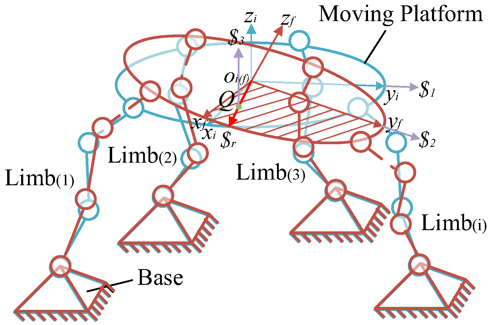
3. Instantaneous Euler Angle of a General Parallel Mechanism

3.1. Assumptions

In this section, a general parallel mechanism is used as an example to illustrate the solution of the instantaneous Euler angle, and the schematic diagram of the general parallel mechanism is introduced in Section 3.2. To facilitate the theoretical analysis, some assumptions are listed below:

• The three rotational DOFs of the general parallel mechanism are considered, and the other three translational DOFs are not considered;
• The rotation of the moving platform is continuous, and the singularities within the cycle are neglected;
• The rotation of the moving platform is a purely rigid rotation; any elastic deformation or micro-displacement is not taken into consideration.

The establishment of the coordinate system is illustrated in Section 3.2. The parallel mechanisms in the blue and red lines represent the initial posture and the final attitude after multiple successive rotations, respectively. The coordinate system O_i-xyz is fixed to the center of the initial attitude of the moving platform, and the coordinate system O_f-xyz is fixed to the center of the final attitude of the moving platform. The red axes indicate the corresponding ridge lines.

3.2. Solution for Each Ridge Axis

(1) Solution of the ridge axis Z_r

First, we denote the ridge axis Z_r as the intersection of the O_ixy plane and the O_fxy plane. As shown in Figure 2, before calculating the position and orientation of the intersection line, the Plücker coordinate of the three lines should be solved. As we mentioned in Section 2, the three lines should be specified as follows: ${\mathsf{\$}}_1$ is denoted as coinciding with the O_fy axis, ${\mathsf{\$}}_2$ is the O_iy axis, and ${\mathsf{\$}}_3$ is the axis that passes through the point Q(Q_x Q_y 0) and parallel with the O_iz axis.

The screw of the three lines can be expressed as:

$$\{\begin{array}{l}{\mathsf{\$}}_{O_{fy}}(t_{03})=(\begin{array}{c}c\alpha \left(t_{01}\right)s\beta \left(t_{02}\right)s\gamma -s\alpha \left(t_{01}\right)c\gamma \left(t_{03}\right)\dots \end{array}\hfill \\ \begin{array}{l}\begin{array}{cc}\dots s\alpha (t_{01})s\beta \left(t_{02}\right)s\gamma \left(t_{03}\right)+c\alpha c\gamma \left(t_{03}\right)& c\beta \left(t_{02}\right)s\gamma \left(t_{03}\right);\begin{array}{ccc}0& 0& 0\end{array}\end{array})\\ {\mathsf{\$}}_{O_{iy}}(t_{03})=\left(\begin{array}{ccc}0& 1& 0\end{array};\begin{array}{ccc}0& 0& 0\end{array}\right)\end{array}\hfill \\ {\mathsf{\$}}_{Q_{iz}}(t_{03})=\left(\begin{array}{ccc}0& 0& 1\end{array};\begin{array}{ccc}{Q}_Y& -Q_X& 0\end{array}\right)\hfill \end{array}$$

(8)

According to the principle of reciprocal products, the axis of the intersection between the plane O_fxy and plane O_ixy can be expressed as:

$${\mathsf{\$}}_{xy}^R(t_{03})=\left(\begin{array}{ccc}{Q}_x\left(t_{03}\right)& Q_y\left(t_{03}\right)& 0\end{array};\begin{array}{ccc}0& 0& 0\end{array}\right)$$

(9)

where the point Q is an arbitrary point on the moving platform appearing on the moment $t_{03}$. The decoupled angle between the O_fxy plane and O_ixy plane can be obtained by calculating the angle between the normal lines of the two planes as:

$${\chi }_z\left(t_{03}\right)=\arccos (c\beta (t_{02}\left)c\gamma \right(t_{03}))$$

(10)

(2) Solution of the ridge axis Y_r

Next, we denote the ridge axis Y_r as the intersection line of O_ixz plane and O_fxz plane. As shown in Figure 3, before calculating the position and orientation of the intersection line, the Plücker coordinate of the three lines should be determined. ${\mathsf{\$}}_1$ is denoted as coinciding with the O_fx axis, ${\mathsf{\$}}_2$ is the O_ix axis, and ${\mathsf{\$}}_3$ is the axis that passes through the point Q(Q_x 0 Q_z) and parallel with the O_iy axis.

The screw of the three lines can be expressed as:

$$\{\begin{array}{l}{\mathsf{\$}}_{O_{fx}}(t_{03})=(c\alpha \left(t_{01}\right)s\beta \left(t_{02}\right)s\gamma \left(t_{03}\right)-s\alpha \left(t_{01}\right)c\gamma \left(t_{03}\right)\dots \hfill \\ \begin{array}{l}\begin{array}{cc}\dots s\alpha (t_{01})s\beta \left(t_{02}\right)s\gamma \left(t_{03}\right)+c\alpha \left(t_{01}\right)c\gamma \left(t_{03}\right)& c\beta \left(t_{02}\right)s\gamma \left(t_{03}\right)\end{array};\begin{array}{ccc}0& 0& 0\end{array})\\ {\mathsf{\$}}_{O_{ix}}(t_{03})=\left(\begin{array}{ccc}0& 1& 0\end{array};\begin{array}{ccc}0& 0& 0\end{array}\right)\end{array}\hfill \\ {\mathsf{\$}}_{Q_{iy}}(t_{03})=\left(\begin{array}{ccc}0& 0& 1\end{array};\begin{array}{ccc}{Q}_Y& -Q_X& 0\end{array}\right)\hfill \end{array}$$

(11)

According to the principle of reciprocal product, the axis of the intersection line of the plane O_fxz and plane O_ixz can be expressed in Plücker coordinates as:

$${\mathsf{\$}}_{xz}^R\left(t_{03}\right)=\left(\begin{array}{ccc}{Q}_x\left(t_{03}\right)& 0& Q_z\left(t_{03}\right)\end{array};\begin{array}{ccc}0& 0& 0\end{array}\right)$$

(12)

The decoupled angle between the O_fxz plane and O_ixz plane can be obtained by calculating the angle between the normal lines of the two planes as:

$${\chi }_y\left(t_{03}\right)=\arccos (s\alpha (t_{01}\left)s\beta \right(t_{02}\left)s\gamma \right(t_{03})+c\alpha (t_{01}\left)c\gamma \right(t_{03}))$$

(13)

(3) Solution of the ridge axis X_r

Third, we denote the ridge axis X_r as the intersection line of the O_iyz plane and O_fyz plane. As shown in Figure 4, before calculating the position and orientation of the intersection line, the Plücker coordinate of the three lines should be determined. ${\mathsf{\$}}_1$ is denoted as coinciding with the O_fz axis, ${\mathsf{\$}}_2$ is the O_iz axis, and ${\mathsf{\$}}_3$ is the axis that passes through the point Q(0 Q_y Q_z) and parallel with the O_ix axis.

The screw of the three lines can be expressed as:

$$\{\begin{array}{l}{\mathsf{\$}}_{O_{fz}}(t_{03})=(c\alpha \left(t_{01}\right)s\beta \left(t_{02}\right)c\gamma \left(t_{03}\right)+s\alpha \left(t_{01}\right)s\gamma \left(t_{03}\right)\dots \hfill \\ \begin{array}{l}\begin{array}{cc}\dots s\alpha \left(t_{01}\right)s\beta \left(t_{02}\right)c\gamma -c\alpha \left(t_{01}\right)s\gamma \left(t_{03}\right)& c\beta \left(t_{02}\right)c\gamma \left(t_{03}\right)\end{array};\begin{array}{ccc}0& 0& 0\end{array})\\ {\mathsf{\$}}_{O_{i\mathrm{z}}}(t_{03})=\left(\begin{array}{ccc}0& 0& 1\end{array};\begin{array}{ccc}0& 0& 0\end{array}\right)\end{array}\hfill \\ {\mathsf{\$}}_{Q_{ix}}(t_{03})=\left(\begin{array}{ccc}1& 0& 0\end{array};\begin{array}{ccc}0& Q_Z& -Q_Y\end{array}\right)\hfill \end{array}$$

(14)

According to the principle of reciprocal products, the axis of the intersection between the O_fyz plane and O_iyz plane can be expressed in Plücker coordinates as:

$${\mathsf{\$}}_{yz}^R\left(t_{03}\right)=\left(\begin{array}{ccc}0& Q_y\left(t_{03}\right)& Q_z\left(t_{03}\right)\end{array};\begin{array}{ccc}0& 0& 0\end{array}\right)$$

(15)

The decoupled angle between the O_fyz plane and O_iyz plane can be obtained by calculating the angle between the normal lines of the two planes:

$${\chi }_x\left(t_{03}\right)=\arccos (c\alpha (t_{01})c\beta (t_{02}))$$

(16)

It is worth noting that the three Euler angles $\alpha$, $\beta$, and $\gamma$ belong to the different time domains, but Equations (10), (13) and (16) transfer the three variables to the same time domain; i.e., they transform the three process variables into three status variables describing the rotation of the parallel mechanism at a particular moment in time.

4. Discussion of the Intrinsic Relationship between the Conventional Euler Angle and the Instantaneous Euler Angle

This section aims to investigate two Euler angle description methods to establish the relationship with the instantaneous Euler angle. In [28], there are 12 combinations of Euler angles used to describe the rotation of a rigid body; most of the sequences can be found to be similar. Since some Euler angles are named in the opposite order of the embryonic names, they have different initial axis directions and positions. Due to the nature of Euler angles, basically only four are typical, namely, ZYX, ZXY, ZYZ, and ZXZ. Among the typical Euler angles, ZYX and ZYZ are selected for analysis in this paper, and their mapping relationships with the corresponding instantaneous Euler angle are obtained.

4.1. Z-Y-Z Euler Angle (Φ, θ, and φ)

For the Z-Y-Z Euler angle, the first rotation is rotated by Φ degrees around the z₀ axis, the second rotation is rotated by θ degrees around the y₁ axis, and the third rotation is rotated by φ degrees around the z₂ axis; the final position can be expressed as o-x₃y₃z₃. When the three Euler angles are known, the final posture [28] of the parallel mechanism can be derived as:

$$\begin{array}{l}Euler\left({\varphi }_z,{\theta }_y,{\phi }_z\right)=\left[R_{\varphi }\right]\left[R_{\theta }\right]\left[R_{\phi }\right]\\ =\left[\begin{array}{ccc}\cos \varphi \cos \theta \cos \phi -\sin \varphi \sin \phi & -\cos \varphi \cos \theta \sin \phi -\sin \varphi \cos \phi & \cos \varphi \sin \theta \\ \sin \varphi \cos \theta \cos \phi +\cos \varphi \sin \phi & -\sin \varphi \cos \theta \sin \phi +\cos \varphi \sin \phi & \sin \varphi \sin \theta \\ -\sin \theta \cos \phi & \sin \theta \sin \phi & \cos \theta \end{array}\right]\end{array}$$

(17)

According to Equations (10), (13) and (16), the mapping relationship between the instantaneous Euler angle and the Z-Y-Z Euler angle can be expressed as:

$$\{\begin{array}{l}{\chi }_x=\theta \\ {\chi }_y=\arccos (-\sin \varphi \cos \theta \sin \phi +\cos \varphi \sin \phi )\\ {\chi }_z=\arccos (\cos \varphi \cos \theta \cos \phi -\sin \varphi \sin \phi )\end{array}$$

(18)

Through Equation (18), we can further investigate the intrinsic relationship of the intersection lines between the Euler angle and the instantaneous Euler angle after multiple successive rotations.

One-time rotation: If the Euler angle is expressed as $\left(\begin{array}{ccc}\alpha & 0& 0\end{array}\right)$, then the corresponding instantaneous Euler angle can be expressed as $\left(\begin{array}{ccc}\alpha & \alpha & 0\end{array}\right)$; i.e., when the ridge axes are expressed as $Z_r$ and $Y_r$, the axis $Z_r$ coincides with the z₀ axis after the first rotation. If the Euler angle is denoted as $\left(\begin{array}{ccc}0& \beta & 0\end{array}\right)$, the corresponding instantaneous Euler angle can be expressed as $\left(\begin{array}{ccc}\beta & 0& \beta \end{array}\right)$, i.e., when the ridge axes are denoted as $Z_r$ and $X_r$, each axis is not coincident with the y₀ axis after the first rotation. If the Euler angle is denoted as $\left(\begin{array}{ccc}0& 0& \gamma \end{array}\right)$, the corresponding instantaneous Euler angle can be expressed as $\left(\begin{array}{ccc}0& \gamma & \gamma \end{array}\right)$; that is, when the ridge axes are denoted as $Y_r$ and $X_r$, the axis $X_r$ coincides with the x₀ axis after the first rotation. It is worth noting that, for the two parallel planes of rotation, the ox₃y₃ plane is parallel to the oxy plane, and two of the three Euler angles are zero, that is, $\beta =\gamma =0$, where each Euler angle represents the attitude of the rotation plane. The expression of the instantaneous Euler angle is the same as the corresponding conventional Euler angle.

Two-time rotation: If the Euler angle is denoted as $\left(0,\beta ,\gamma \right)$, the corresponding instantaneous Euler angle can be expressed as $\left(\begin{array}{ccc}\beta & \gamma & \arccos (\cos \beta \cos \gamma )\end{array}\right)$, and the ridge axes are denoted as $Z_r$ and $Y_r$, where each axis appears after the second rotation. If the Euler angle is denoted as $\left(\alpha ,\beta ,0\right)$, the corresponding instantaneous Euler angle can be expressed as $\left(\begin{array}{ccc}\arccos (\cos \alpha \cos \beta )& \alpha & \beta \end{array}\right)$, and the ridge axes are denoted as $Z_r$, $Y_r$, and $X_r$, where each axis appears after the second rotation. If the Euler angle is denoted as $\left(\alpha ,0,\gamma \right)$, the corresponding instantaneous Euler angle can be expressed as $\left(\begin{array}{ccc}\alpha & \arccos (\cos \alpha \cos \gamma )& \gamma \end{array}\right)$, and the ridge axes are denoted as $X_r$ and $Y_r$, where each of the axes appear after the second rotation.

Three-time rotation: If the Euler angle is denoted as $\left(\alpha ,\beta ,\gamma \right)$, the corresponding instantaneous Euler angle can be expressed as Equation (18), and the ridge axes are denoted as $Z_r$, $Y_r$, and $X_r$, where each axis appears after the third rotation.

4.2. Z-Y-X Euler Angle (α, β, γ)

For the Z-Y-X Euler angle, the first rotation is rotated by $\alpha$ degrees around the z₀ axis, the second rotation is rotated by $\beta$ degrees around the y₁ axis, and the third rotation is rotated by $\gamma$ degrees around the x₂ axis; the final position can be expressed as o-x₃y₃z₃. When the three Euler angles are known, the final posture [28] of the parallel mechanism can be derived as:

$$\begin{array}{l}Euler\left({\alpha }_z,{\beta }_y,{\gamma }_x\right)=\left[R_{\alpha }\right]\left[R_{\beta }\right]\left[R_{\gamma }\right]\\ =\left[\begin{array}{ccc}\cos \alpha \cos \beta & \cos \alpha \sin \beta \sin \gamma -\sin \alpha \cos \gamma & \cos \alpha \sin \beta \cos \gamma +\sin \alpha \sin \gamma \\ \sin \alpha \cos \beta & \sin \alpha \sin \beta \sin \gamma +\cos \alpha \cos \gamma & \sin \alpha \sin \beta \cos \gamma -\cos \alpha \sin \gamma \\ -\sin \beta & \cos \beta \sin \gamma & \cos \beta \cos \gamma \end{array}\right]\end{array}$$

(19)

According to Equations (10), (13) and (16), the mapping relationship between the instantaneous Euler angle and Z-Y-X Euler angle can be expressed as:

$$\{\begin{array}{l}{\chi }_x=\arccos (\cos \beta \cos \gamma )\\ {\chi }_y=\mathrm{acos}\left(\sin \alpha \sin \beta \sin \gamma +\cos \alpha \cos \gamma \right)\\ {\chi }_z=\mathrm{acos}\left(\cos \alpha \cos \beta \right)\end{array}$$

(20)

In the same way, we can investigate the intrinsic relationship of the intersection lines between the Euler angle and the instantaneous Euler angle after multiple consecutive rotations by Equation (20).

One-time rotation: If the Euler angle is expressed as $\left(\begin{array}{ccc}\varphi & 0& 0\end{array}\right)$, the corresponding instantaneous Euler angle can be expressed as $\left(\begin{array}{ccc}\varphi & 0& 0\end{array}\right)$; that is, when the ridge axis is expressed as $Z_r$, the axis coincides with the z₁ axis after the first rotation. If the Euler angle is expressed as $\left(\begin{array}{ccc}0& \theta & 0\end{array}\right)$, the corresponding instantaneous Euler angle can be expressed as $\left(\begin{array}{ccc}\theta & 0& \theta \end{array}\right)$; that is, when the ridge axes are represented as $Z_r$ and $X_r$, the axis $Z_r$ coincides with the y₂ axis after the first time rotation. If the Euler angle is expressed as $\left(\begin{array}{ccc}0& 0& \phi \end{array}\right)$, the corresponding instantaneous Euler angle can be expressed as $\left(\begin{array}{ccc}0& \arccos (\sin \phi )& \phi \end{array}\right)$; that is, when the ridge axes are represented as $Y_r$ and $X_r$, the axis $X_r$ coincides with the z₃ axis by the first time rotation. When the ox₃y₃ plane is parallel to the ox₀y₀ plane, the Euler angle $\theta$ should be equal to zero. If the Euler angle can be expressed as $\left(\begin{array}{ccc}\varphi & 0& 0\end{array}\right)$, the rotation plane is rotated by $\varphi$ degrees around the z₀ axis; if the Euler angle can be expressed as $\left(\begin{array}{ccc}{\varphi }^{\prime }& 0& {\phi }^{\prime }\end{array}\right)$, the rotation plane is rotated by ${\varphi }_3$ degrees around the z₀ axis, and then is rotated by ${\phi }_3$ degrees around z₂ axis. ${\varphi }_3$ and ${\phi }_3$ can be arbitrary values. When the equation ${\theta }^{\prime }+{\phi }^{\prime }=\theta =\phi$ is satisfied, the three descriptions of the instantaneous Euler angle and the Euler angle are the same.

Two-time rotation: If the Euler angle is expressed as $\left(0,\theta ,\phi \right)$, the corresponding instantaneous Euler angle can be expressed as $\left(\begin{array}{ccc}\arccos (\sin \theta \cos \phi )& \phi & \theta \end{array}\right)$; that is, when the ridge axes are denoted as $Z_z$, $Y_r$, and $X_r$, the ridge axis $X_r$ coincides with the original z₃ axis by the second rotation. If the Euler angle is expressed as $\left(\varphi ,\theta ,0\right)$, the corresponding instantaneous Euler angles can be expressed as $\left(\begin{array}{ccc}\arccos (\cos \varphi \cos \theta )& \varphi & \theta \end{array}\right)$; that is, when the ridge axes are denoted as $Z_r$, $Y_r$, and $X_r$, the ridge axis $X_r$ coincides with the original y₃ axis after the second rotation. If the Euler angle is denoted as $\left(\varphi ,0,\phi \right)$, the corresponding instantaneous Euler angle can be expressed as $\left(\begin{array}{ccc}\arccos (\cos \varphi \cos \phi )& \varphi +\phi & 0\end{array}\right)$; that is, when the ridge axes are represented as $X_r$, $Y_r$, and $Z_r$, each axis is not coincident with the original axis after the second rotation.

Three-time rotation: If the Euler angle is expressed as $\left(\varphi ,\theta ,\phi \right)$, the corresponding instantaneous Euler angle can be expressed as Equation (20); that is, when the ridge axes are denoted as $Z_r$, $Y_r$, and $X_r$, each axis is not coincident with the original axis after the third rotation (exception for peculiar circumstances).

Obviously, for the Z-Y-X and Z-Y-Z Euler angles, the instantaneous Euler angle is the arccosine of the diagonal element of the rotation transformation matrix. Therefore, in order to obtain the instantaneous Euler angle, it is necessary to derive the corresponding rotational transformation matrix and obtain the instantaneous Euler angle by calculating the arccosine of the diagonal element of the transformation matrix. The corresponding intersection line can be derived using Equations (10), (13) and (16). By comparing the descriptions of the instantaneous Euler angle and the conventional Euler angle, the difference is that the former represents the change from the initial position to the final position, and each angle belongs to the same time domain, i.e., the instantaneous Euler angle is determined if the final attitude of the rotation plane is specified, regardless of the corresponding changes in Euler angles. On the contrary, if the final attitude of the rotation plane is specified, the Euler angles are not uniquely determined. Therefore, it is concluded that the instantaneous Euler angles proposed in this paper are more suitable than conventional Euler angles to describe the decoupled rotation performance, especially when the instantaneous kinstate of a parallel mechanism needs to be known.

5. Application of the Instantaneous Euler Angle

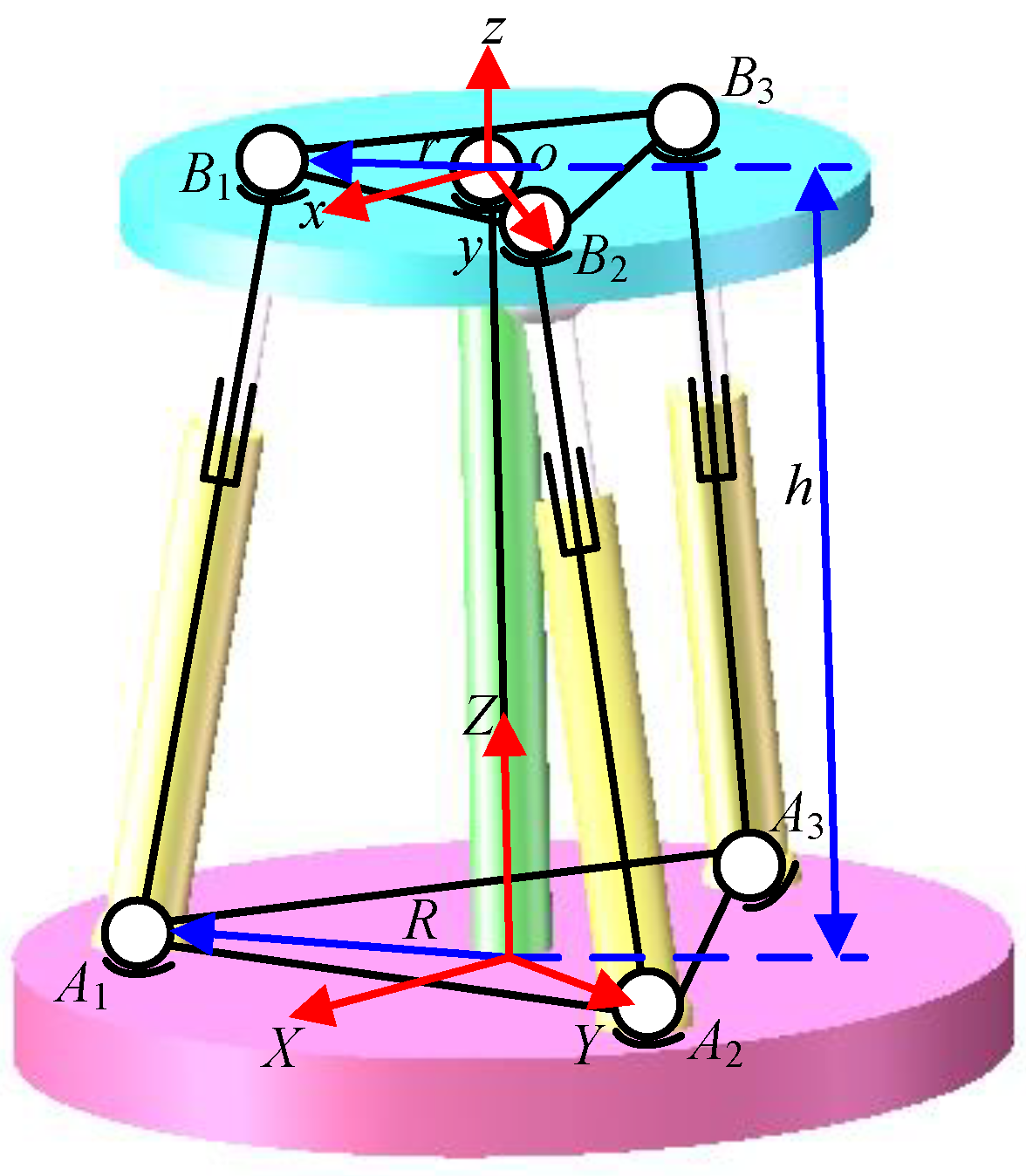
5.1. 3-sps-s Parallel Mechanism

To illustrate the application of the instantaneous Euler angle, a 3-sps-s parallel mechanism is introduced to describe and analyze the spatial rotation of the parallel mechanism.

As shown in Figure 5, the local coordinate system is fixed on the center of the MP, the origin coincides with the center of the MP, and the y-axis coincides with the vector $\overrightarrow{o{B}_2}$. The reference coordinate system is fixed at the center of the base, and the origin coincides with the center of the base. r is the outer radius of MP, R is the outer radius of the base, and the vertical dimension between MP and base is h. MP rotates in the order of z-y-x, and the corresponding Euler angles are α, β, and γ. According to Figure 5, the coordinates of each of the points can be expressed as:

$$B_1^o=r\left[\begin{array}{c}\frac{\sqrt{3}}{2}\\ \frac{1}{2}\\ 0\\ \end{array}\right],B_2^o=r\left[\begin{array}{c}0\\ 1\\ 0\end{array}\right],B_3^o=r\left[\begin{array}{c}-\frac{\sqrt{3}}{2}\\ \frac{1}{2}\\ 0\\ \end{array}\right];A_1^O=R\left[\begin{array}{c}\frac{\sqrt{3}}{2}\\ \frac{1}{2}\\ 0\\ \end{array}\right],A_2^O=R\left[\begin{array}{c}0\\ 1\\ 0\end{array}\right],A_3^O=R\left[\begin{array}{c}-\frac{\sqrt{3}}{2}\\ \frac{1}{2}\\ 0\\ \end{array}\right];$$

(21)

According to the equation $B_i^O=R_o^O{B}_i^O+o^O$, the following results can be obtained:

$$B_i^O=\frac{1}{2}\left[\begin{array}{c}\sqrt{3}r{n}_{11}-r{n}_{12}\\ \sqrt{3}r{m}_{21}-r{m}_{22}\\ \sqrt{3}r{k}_{31}-r{k}_{32}+2h\end{array}\right]; B_2^O=\left[\begin{array}{c}r{n}_{12}\\ r{m}_{22}\\ r{k}_{32}+h\end{array}\right]; B_3^O=\frac{1}{2}\left[\begin{array}{c}-\sqrt{3}r{n}_{11}-r{n}_{12}\\ -\sqrt{3}r{m}_{21}-r{m}_{22}\\ -\sqrt{3}r{k}_{31}-r{k}_{32}+2h\end{array}\right];$$

(22)

Thus, if the rotation angles (α, β, γ) are specified, the corresponding changes in the prismatic joint will be realized, i.e., the mapping relationship between the MP and each active joint is determined as:

$$L_i=\left|B_i^O-A_i^O\right|={\left|{\left(X_{Bi}-X_{Ai}\right)}^2+{\left(Y_{Bi}-Y_{Ai}\right)}^2+{\left(Z_{Bi}-Z_{Ai}\right)}^2\right|}^{1/2}$$

(23)

According to Equations (21)–(23), the instantaneous Euler angles are obtained. The comparison of the simulation between the conventional Euler angle (blue line) and the corresponding instantaneous Euler angle (red line) (see Figure 6) can be analyzed as shown in the following figures.

Assuming that the conventional Euler angles α, β, and γ vary from 0° to 360°, the curve variation indicates that the corresponding instantaneous Euler angles do not follow the conventional Euler angles, and the peaks of the instantaneous Euler angles are smaller than the conventional Euler angles. In addition, for a periodic variation in the Euler angles, the corresponding instantaneous Euler angles tend to be zero, which is more in line with the actual situation. The instantaneous Euler angles correspond to the Euler angles α and γ passing through the origin twice in the cycle, and the instantaneous Euler angle β passing through the origin three times in the cycle. The instantaneous Euler angle describes the angle between the current rotation plane and the initial rotation plane, which is independent of the rotation in other directions at any time. The advantage of this is that the instantaneous Euler angle can be used to describe the absolute rotation value of a rotation direction without considering the coupling of rotation angles in other directions.

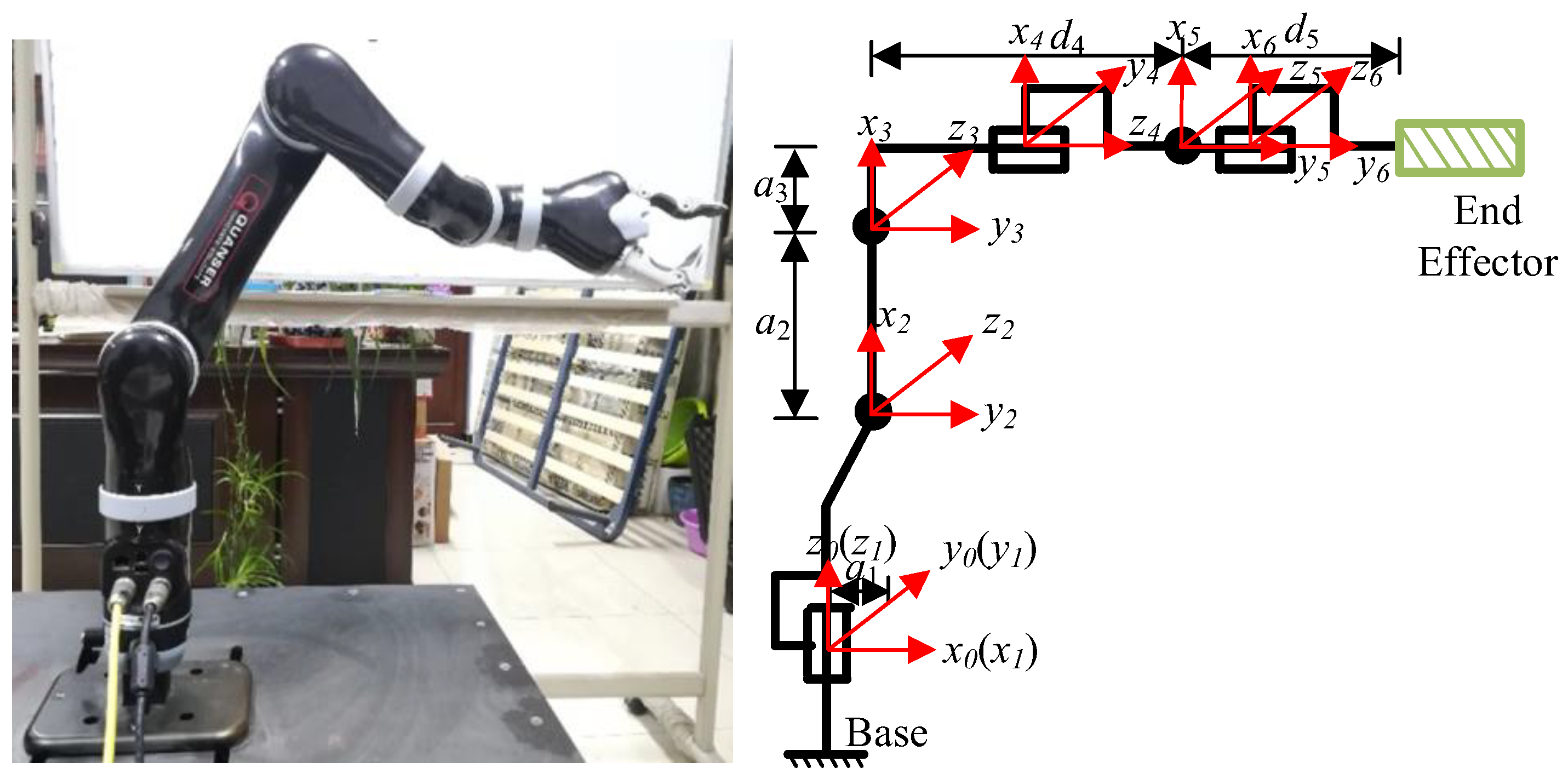
5.2. 6-DOF Robotic Arm

In order to further illustrate the application of the instantaneous Euler angle, a 6-DOF robotic arm is introduced to describe and analysis of the spatial rotation performance. As shown in Figure 7, the local coordinate system is fixed at the center of the base, and the reference coordinate system is fixed at the center of the joint. The rotation plane rotates in the sequence Z-Y-X, and the corresponding Euler angles are α, β, and γ, respectively. The rotation planes XY, YZ, and XZ in the end effector are the rotation planes that are to be investigated. The variation in the Euler angle (blue line) and its corresponding instantaneous Euler angle (green line) are shown for different curves:

Curve 1 $\{\begin{array}{c}\alpha =\sin (x)\\ \beta =0\\ \lambda =0\end{array}$

For curve 1, when the distribution of the angle $\alpha$ varies as a sinusoidal function and the other two Euler angles are zero, it can been observed that the instantaneous Euler angle corresponding to the x axis is equal to the absolute value of $\alpha$; the instantaneous Euler angle corresponding to the y axis is consistent with the instantaneous Euler angle corresponding to the x axis; and the instantaneous Euler angle corresponding to the z axis is 0. It can be seen that when a certain rotation angle changes, other rotation planes will also produce a corresponding coupling rotation angle, which should also be taken into account in the calculation (as shown in Figure 8).

Curve 2 $\{\begin{array}{c}\alpha =\sin (x)\\ \beta =\cos (x)\\ \lambda =0\end{array}$

For curve 2, when the distribution of the angle $\alpha$ varies as a sinusoidal waveform, $\beta$ varies in cosinoidal waveform, and $\lambda$ is zero. It can be observed that the instantaneous Euler angle corresponding to the x axis is greater than the value of $\alpha$; the instantaneous Euler angle corresponding to the y axis varies in sinusoidal waveform; and the instantaneous Euler angle corresponding to the z axis is equal to the absolute value of the angle $\alpha$. Compared with Figure 8, it can be seen that the variation in the Euler angles has an influence on the instantaneous Euler angles; that is, the variation in any instantaneous Euler angle is jointly determined by the other three Euler angles, which shows that the instantaneous Euler angle is a state quantity, denoting the description of the rotation performance of the robot at a certain moment (As shown in Figure 9).

For the successive rotation of some kinds of robots, it is often necessary to describe the rotation angle in three directions at a certain time separately. At this time, the three instantaneous Euler angles are better for the quantifiable description of multiple successive rotations than the conventional Euler angles. During the period of motion, the instantaneous Euler angles are more in line with the actual situation in the simulation. Significantly, the three variables differ from the conventional Euler angle in that the three variables are in the same time domain and independent of each other, which means that they are better suited to describing the decoupled rotation of the robot.

6. Conclusions

In the present study, a novel time domain decoupling method was introduced for managing the multiple consecutive rotations of robots. The proposed approach leverages the instantaneous Euler angle for effective implementation. Through the application of the reciprocal products principle within screw theory, the intersection line between the pre- and post-rotation planes of a generic parallel mechanism is resolved. At the same time, the instantaneous Euler angles are obtained. Additionally, the mathematical mapping relationship and the difference between the instantaneous Euler angle and the Z-Y-X and Z-Y-Z Euler angles were explored. The instantaneous Euler angle was found to be the arccosine of the diagonal element of the rotation transformation matrix of the conventional Euler angle. Through an analysis of the rotational behavior exhibited by two distinct robot types, the fundamental principle and benefits of utilizing the instantaneous Euler angle for depicting consecutive robot rotations were elucidated. As a result, the effectiveness of the method was substantiated to a certain degree. In conclusion, the method provides a theoretical basis for structural synthesis, performance evaluation, and parameter optimization in the field of robotics.

References

1. Li, K.; Jiang, H.; Wang, S.; Yu, J. A soft robotic fish with variable stiffness decoupled mechanisms. J. Bionic Eng. 2018, 15, 599–609. [Google Scholar] [CrossRef]
2. Abduh, W.; Berhouet, J.; Samargandi, R.; Favard, L. Clinical results and radiological bony adaptations on a cementless short-stem prosthesis-a comparative study between anatomical and reverse total shoulder arthroplasty. Orthop. Traumatol. Surg. Res. 2022, 108, 103262. [Google Scholar] [CrossRef] [PubMed]
3. Acar, O.; Şaka, Z.; Özçelik, Z. Parametric Euler-Savary Equations for Spherical instantaneous Kinematics, Mechanisms and Machine Science; Springer: Berlin/Heidelberg, Germany, 2019; pp. 347–356. [Google Scholar]
4. Balakina, E.A.; Kuznetsov, E.B. On the numerical integration of the Euler kinematic Equations. Comput. Math. Math. Phys. 2001, 41, 1623–1629. [Google Scholar]
5. Li, K.; Zhang, Y.; Zhan, H.; Du, Y.; Lü, C. Vibrational characteristics of rotating soft cylinders. Sci. China-Phys. Mech. Astron. 2021, 64, 254611. [Google Scholar] [CrossRef]
6. Giulietti, F.; Tortora, P. Optimal Rotation Angle about a Nonnominal Euler Axis. J. Guid. Control. Dyn. 2007, 30, 1561–1563. [Google Scholar] [CrossRef]
7. Lovera, M.; Astolfi, A. Spacecraft Attitude Control Using Magnetic Actuators. Automatica 2004, 40, 1405–1414. [Google Scholar] [CrossRef]
8. Araromi, O.A.; Gavrilovich, I.; Shintake, J.; Rosset, S.; Richard, M.; Gass, V.; Shea, H.R. Rollable Multisegment Dielectric Elastomer Minimum Energy Structures for a Deployable Microsatellite Gripper. IEEE/ASME Trans. Mechatron. 2014, 20, 438–446. [Google Scholar] [CrossRef]
9. Zhu, T.; Liu, Y.; Li, W.; Li, K. The quaternion-based attitude error for the nonlinear error model of the INS. IEEE Sens. J. 2021, 21, 25782–25795. [Google Scholar] [CrossRef]
10. Shuster, M.D.; Oh, S.D. Three-Axis Attitude Determination from Vector Observation. J. Guid. Control Dyn. 1981, 4, 70–77. [Google Scholar] [CrossRef]
11. Ershkov, S.V. New exact solution of Euler’s Equations (rigid body dynamics) in the case of rotation over the fixed point. Arch. Appl. Mech. 2014, 84, 385–389. [Google Scholar] [CrossRef]
12. Behal, A.; Dawson, D.; Zergeroglu, E.; Fang, Y. Nonlinear Tracking Control of an Underactuated Spacecraft. J. Guid. Control. Dyn. 2002, 25, 979–985. [Google Scholar] [CrossRef]
13. Baoyin, H.; Yin, M. Review on time-optimal reorientation of agile satellite. J. Dyn. Control 2020, 18, 1–11. (In Chinese) [Google Scholar]
14. Bonev, I.A.; Gosselin, C. Advantages of the modified euler angles in the design and control of PKMs. In Proceedings of the 2002 Parallel Kinematic Machines International Conference, Montreal, QC, Canada, 23–25 April 2002; pp. 171–188. [Google Scholar]
15. Taunyazov, T.; Rubagotti, M.; Shintemirov, A. Constrained orientation control of a spherical parallel manipulator via online convex optimization. IEEE/ASME Trans. Mechatron. 2017, 23, 252–261. [Google Scholar] [CrossRef]
16. Cao, Z.; Qin, C.; Fan, S.; Yu, D.; Wu, Y.; Qin, J.; Chen, X. Pilot study of a surgical robot system for zygomatic implant placement. Med. Eng. Phys. 2020, 75, 72–78. [Google Scholar] [CrossRef] [PubMed]
17. Feng, Y.; Fan, J.; Tao, B.; Wang, S.; Mo, J.; Wu, Y.; Liang, Q.; Chen, X. An image-guided hybrid robot system for dental implant surgery. Int. J. Comput. Assist. Radiol. Surg. 2022, 17, 15–26. [Google Scholar] [CrossRef]
18. Hu, H.; Cheng, J.; Niu, Z. Analysis on obstacle-surmounting of coal mine detection robot based on RPY. J. Coal Mine Mach. 2013, 34, 109–111. [Google Scholar]
19. Wei, L.; Toby, H.; Jorge, A. On the use of the dual euler-rodrigues parameters in the numerical solution of the inverse-displacement problem. Mech. Mach. Theory 2018, 125, 21–33. [Google Scholar]
20. Yazell, D. Origins of the unusual space shuttle quaternion definition. In Proceedings of the 47th American Institute of Aeronautics and Astronautics, Orlando, FL, USA, 5–9 January 2009; Volume 43, pp. 1–6. [Google Scholar]
21. Wang, X.; Yu, C.; Lin, Z. A dual quaternion solution to attitude and position control for rigid-body coordination. IEEE Trans. Robot. 2012, 28, 1162–1170. [Google Scholar] [CrossRef]
22. Biswal, P.; Mohanty, P.K. Development of quadruped walking robots: A review. Ain Shams Eng. J. 2021, 12, 2017–2031. [Google Scholar] [CrossRef]
23. Mofid, O.; Mobayen, S.; Zhang, C.; Esakki, B. Desired tracking of delayed quadrotor UAV under model uncertainty and wind disturbance using adaptive super-twisting terminal sliding mode control. ISA Trans. 2022, 123, 455–471. [Google Scholar] [CrossRef]
24. Hua, C.C.; Wang, K.; Chen, J.N.; You, X. Tracking differentiator and extended state observer -based nonsingular fast terminal sliding mode attitude control for a quadrotor. Nonlinear Dyn. 2018, 94, 343–354. [Google Scholar] [CrossRef]
25. Khoder, W.; Fassinut-Mombot, B.; Benjelloun, M. Inertial navigation attitude velocity and position algorithms using quaternion scaled unscented kalman filtering. In Proceedings of the IEEE Industrial Electronics, Orlando, FL, USA, 10–13 November 2008; pp. 754–759. [Google Scholar]
26. Luo, J.; Wei, C.; Dai, H.; Yin, Z.; Wei, X.; Yuan, J. Robust inertia-free attitude takeover control of post capture combined spacecraft with guaranteed prescribed performance. ISA Trans. 2018, 74, 28–44. [Google Scholar] [CrossRef] [PubMed]
27. Zhang, D.; Yao, J.; Xu, Y.; Duan, Y.; Hou, Y.; Zhao, Y. The Internal Relations of the Pose Description Methods of the Rigid Body after Two Successive Rotations. J. Mech. Eng. 2015, 51, 86–94. [Google Scholar] [CrossRef]
28. Zhen, H.; Yanwen, L.; Feng, G. The expression of the orientation of a spatial moving unit by Euler angle. J. Yanshan Univ. 2002, 26, 189–192. [Google Scholar]
29. Qu, S.; Li, R.; Bai, S. Type Synthesis of 2T1R Decoupled Parallel Mechanisms Based on Lie Groups and Screw Theory. Math. Probl. Eng. 2017, 2017, 8304312. [Google Scholar] [CrossRef]
30. Kong, X.W.; Gosselin, C.M. Type Synthesis of Input-Output Decoupled Parallel Manipulators. Trans. Can. Soc. Mech. Eng. 2004, 28, 185–196. [Google Scholar] [CrossRef]
31. Li, C.; Guo, H.; Tang, D. Cell division method for mobility analysis of multi-loop mechanisms. Mech. Mach. Theory 2019, 141, 67–94. [Google Scholar] [CrossRef]
32. Li, W.; Gao, F.; Zhang, J. A Decoupled Parallel Manipulator only with Revolute Joints. Mech. Mach. Theory 2005, 40, 467–473. [Google Scholar] [CrossRef]
33. Liu, X.; Wu, C.; Wang, J.; Bonev, I. Attitude description method of [PP]S type parallel robotic mechanisms. Chin. J. Mech. Eng. 2008, 44, 19–23. [Google Scholar] [CrossRef]
34. Jack, P. Freedom in Machinery; Cambridge University Press: Sydney, Australia, 1900; pp. 1–30. [Google Scholar]
Figure 1. Variation in the Euler angles in time domain.
Mathematics 11 03882 g001
Figure 2. Diagram of the screw’s distribution for three-time rotation (for intersection line between the Oixy plane and Ofxy plane).
Mathematics 11 03882 g002
Figure 3. Schematic diagram of the distribution of the three rotating screws (for the intersection line between the Oixz plane and Ofxz plane).
Mathematics 11 03882 g003
Figure 4. Schematic diagram of the distribution of the three rotating screws (for the intersection line between the Oiyz plane and Ofyz plane).
Mathematics 11 03882 g004
Figure 5. Schematic diagram of the 3-sps-s parallel mechanism.
Mathematics 11 03882 g005
Figure 6. Analysis of the variation in the conventional Euler angle and the corresponding instantaneous Euler angle.
Mathematics 11 03882 g006
Figure 7. Schematic diagram of the robotic arm.
Mathematics 11 03882 g007
Figure 8. (a) Comparison between the instantaneous Euler angle and its corresponding Euler angle α. (b) Comparison between the instantaneous Euler angle and its corresponding Euler angle β. (c) Comparison between the instantaneous Euler angle and its corresponding Euler γ.
Mathematics 11 03882 g008
Figure 9. (a) Comparison between the instantaneous Euler angle and its corresponding Euler angle α. (b) Comparison between the instantaneous Euler angle and its corresponding Euler angle β. (c) Comparison between the instantaneous Euler angle and its corresponding Euler angle γ.
Mathematics 11 03882 g009
Disclaimer/Publisher’s Note: The statements, opinions and data contained in all publications are solely those of the individual author(s) and contributor(s) and not of MDPI and/or the editor(s). MDPI and/or the editor(s) disclaim responsibility for any injury to people or property resulting from any ideas, methods, instructions or products referred to in the content.