Article

Multistage Adaptive Robust Binary Optimization: Uncertainty Set Lifting versus Partitioning through Breakpoints Optimization

Department of Chemical & Materials Engineering, University of Alberta, Edmonton, AB T6G 1H9, Canada
*
Author to whom correspondence should be addressed.
Mathematics 2023, 11(18), 3883; https://doi.org/10.3390/math11183883
Submission received: 22 August 2023 / Revised: 4 September 2023 / Accepted: 9 September 2023 / Published: 12 September 2023
(This article belongs to the Section Engineering Mathematics)

Abstract

:
Two methods for multistage adaptive robust binary optimization are investigated in this work. These methods referred to as binary decision rule and finite adaptability inherently share similarities in dividing the uncertainty set into subsets. In the binary decision rule method, the uncertainty is lifted using indicator functions which result in a nonconvex lifted uncertainty set. The linear decision rule is further applied to a convexified version of the lifted uncertainty set. In the finite adaptability method, the uncertainty set is divided into partitions and a constant decision is applied for each partition. In both methods, breakpoints are utilized either to define the indicator functions in the lifting method or to partition the uncertainty set in the finite adaptability method. In this work, we propose variable breakpoint location optimization for both methods. Extensive computational study on an illustrating example and a larger size case study is conducted. The performance of binary decision rule and finite adaptability methods under fixed and variable breakpoint approaches is compared.

1. Introduction

Multistage decision making under uncertainty has practical applications in many areas such as finance, engineering, and operations management, etc. To mention a few examples, Goulart et al. [1] applied stochastic optimization for the robust control of linear discrete-time systems. Skaf and Boyd [2] designed an affine controller for linear dynamic systems. Ben Tal et al. [3] addressed the problem of minimizing the overall cost of a supply chain under demand uncertainty. See and Sim [4] proposed a robust optimization method to tackle an inventory control problem where only limited demand information is available. Gounaris et al. [5] studied the robust vehicle routing problem to minimize the delivery costs of a product to geographically dispersed customers using capacity-constrained vehicles. Calafiore [6] presented an affine control method for dynamic asset allocation. Fadda et al. [7] studied the multi-period stochastic assignment problem for social engagement.
There are challenges to solving multistage adaptive robust optimization problems. As Shapiro and Nemirovski [8] pointed out, multistage adaptive robust optimization problems including real-valued and binary decision variables are computationally intractable in general. Dyer and Stougie [9] demonstrated that obtaining the optimal solution for the class of single-stage uncertain problems involving only real-valued decisions is already P-hard. One popular solution approach to this problem is to use decision rules where variables are modeled as functions of uncertain parameters. The application of decision rules for real-valued functions in stochastic programming goes back to 1974 [10]. However, only recently did the decision rule-based approach received major attention with the research advances made in robust optimization [11,12]. Ben-Tal et al. [13] formulated the real-valued functions as affine functions of uncertain parameters. The simple structure of linear decision rules may result in some optimality loss. However, it has the advantage of providing the required scalability to deal with multistage stochastic adaptive problems. It should be mentioned that linear decision rules are shown to be optimal in some problem instances. For instance, Bertsimas et al. [14] showed the optimality of affine control policies in one-dimensional uncertainty within robust optimization context. The reader can refer to [5,15] for other cases.
In order to reduce the loss of optimality due to linear decision rules, various nonlinear decision rule structures were proposed. Motivated by the success of linear decision rules in providing the favorable scalability features for multistage problems, the nonlinear decision rules are formulated as x ( ξ ) = X O ( ξ ) where x is the decision variable, ξ denotes the uncertain parameters, X represents the decision rule coefficients, and O : R m R m is a nonlinear operator that defines the basis terms in the decision rule. This structure considerably improves the solution optimality while retaining the scalability property. To mention some instances, different authors have suggested various decision rule structures such as linear [1,2,13,16], piecewise linear [17,18,19,20], multilinear [19], quadratic [19,21] and polynomial. Kuhn et al. [16] proposed a method to estimate the approximation error introduced by linear decision rules. They have argued the method is applicable to problems with random recourse and multiple decision stages. Chen et al. [17] addressed uncertain problems where only limited information of underlying stochastic parameters are available. The authors discussed that linear decision rules are inadequate for this type of problem and can result in infeasible solutions. They suggested an alternative second-order conic optimization model that can be solved efficiently. Chen and Zhang [18] presented an extended affinely adjustable robust counterpart method to solve multistage uncertain linear problems and illustrated that the potential of their proposed method is beyond what is presented in the literature. Georghiou et al. [19] proposed a lifting technique that provides tighter upper and lower bounds compared to the case where the linear decision rule is directly applied to the original stochastic problem. They proposed a structured lifting method that gives rise to a flexible piecewise linear and nonlinear decision rules. Goh and Sim [20] developed new piecewise linear decision rules that provide a more flexible formulation of the original uncertain problem and results in better bounds on the objective. Bertsimas et al. [22] proposed a framework for tackling linear dynamic systems under uncertainty. They introduced a hierarchy of polynomial control policies that exhibited strong numerical performance at a moderate computational expense.
Although there is a wealth of literature available for real-valued decision rules, the available literature for binary decision rules is relatively scarce. Bertsimas and Georghiou [23] proposed a structure for binary decision rules that models binary variables as piecewise constant functions and can provide high-quality solutions. However, the computational expense is significant. Bertsimas and Caramanis [24] proposed a structure for integer decision rules formulated as y ( ξ ) = y ξ , where y Z k and · is the ceiling function. In their work, the resulting problem is approximated and solved using a randomized algorithm [25] that provides only a limited guarantee on solution feasibility. Hanasusanto et al. [26] proposed a so-called “k-adaptable” structure that can only be applied to two-stage uncertain binary problems where the decision maker pre-commits to k second-stage policies and implements the best one once the uncertain parameters are revealed. Recently, Bertsimas and Georghiou [27] proposed a systematic lifting method for binary decision rule that trades off scalability and optimality. This method can be applied to large multistage problems. They demonstrated that the method is highly scalable and provides high-quality solutions and can readily be used along with real-valued decision rules with the general structure of x ( ξ ) = x O ( ξ ) , O : R m R m . Postek and Den Hertog [28] proposed a method to iteratively split the uncertainty set into subsets based on some heuristics. The method keeps the computational complexity at the same level as the static robust optimization problem. Bertsimas and Dunning [29] extended the work of finite adaptability and presented a partition-and-bound method for the multistage adaptive robust mixed integer optimization problem.
While there are many possible ways for uncertainty lifting and uncertainty set partition, we focus on the grid partition-based method in this work considering its simplicity in implementation. This means that for the lifting method, we lift each uncertain parameter individually instead of any aggregated version among them. Whereas, for the uncertainty set partition method, we divide the uncertainty set using hyper-rectangles. Under this assumption, the binary decision rule (lifting) method and the finite adaptability method (with grid partitioning) for addressing multistage adaptive robust optimization problems inherently share similarities. The goal of this study is to compare the solution complexity of these two methods in order to obtain insights into the advantages and limitations of each method. The contribution of this work is summarized below:
  • Point out the similarity and difference between the lifting method and the finite adaptability (partitioning) method. We demonstrate that under the equivalent setting, the partition method in general leads to better solution quality since the lifting method has less flexibility due to the restriction of linear decision rule.
  • Propose novel breakpoint optimization formulations for both lifting and partitioning methods. It is shown that breakpoint optimization leads to improved solution quality with the cost of solving mixed integer nonlinear problems (MINLP) compared to mixed integer linear problems (MILP) under a fixed breakpoint setting.
  • Conduct an extensive computational study to investigate the advantages of lifting and finite adaptability methods under fixed breakpoint and variable breakpoint settings. We highlight the tractability of the lifting method for handling large cases with many time stages, and the limitation of finite adaptability method caused by the quick increase in model size.
This paper is organized as follows. Section 2 presents the general multistage adaptive robust binary optimization problem formulation and the traditional scenario tree-based method is applied to an illustrating example. Section 3 provides detailed formulations of the binary decision rule method based on the lifting technique and the variable breakpoint technique is explained. Section 4 provides the detailed formulation for the finite adaptability method based on uncertainty set partitioning and the variable breakpoint-based formulation is presented. Section 5 presents an extensive computational study using an inventory control problem and finally, Section 6 concludes the paper.

2. Multistage Adaptive Robust Binary Optimization

The multistage adaptive robust binary optimization problem to be addressed is as follows:
min E ξ t ( D t ξ [ t ] ) y t ( ξ [ t ] )
s . t . τ = 1 t B t , τ y τ ( ξ [ τ ] ) E t ξ [ t ] ξ Ξ , t = 1 , . . . , T
y t ( ξ [ t ] ) { 0 , 1 } N y t
where D t , B t , τ and E t are constant vectors/matrices, y t ( ξ [ t ] ) is the adaptive binary decision variable expressed as a function of uncertainty vector ξ [ t ] , based on the following notation:
ξ q , t scalar, q-th uncertain parameter of stage t
ξ t vector of uncertain parameters of stage t: [ ξ 1 , t , , ξ q t ¯ , t ] ,
 where q t ¯ is the number of uncertain parameters in stage t
ξ [ t ] vector of uncertain parameters from stage 1 to t: 1 , ξ 1 , , ξ t
ξ vector of all uncertain parameters (from stage 1 to T): 1 , ξ 1 , , ξ T , that is, ξ [ T ]
In this work, we consider polyhedral uncertainty set for ξ R | ξ [ T ] | ( | ξ [ T ] | is the size of ξ ):
Ξ = { ξ : J ξ h }
where J and h are the constant matrix and vector, respectively. For each uncertain parameter, we assume that it is subject to an interval Ξ q , t = { ξ ̲ q , t ξ q , t ξ ¯ q , t } .
Illustrating example
Throughout this paper, we will study the following illustrating example while presenting various solution methods. The problem has two stages (t = 1, 2). Each stage includes only one uncertain parameter. First stage decision y 1 could depend on ξ 1 , and the second stage decision y 2 could depend on both ξ 1 and ξ 2 . The problem is formulated as:
min E ξ ( y 1 ( ξ ) y 2 ( ξ ) )
s . t . 2 y 1 ( ξ ) 1 + 2 ξ 1 ξ Ξ
3 y 1 ( ξ ) + 2 y 2 ( ξ ) 1 + 2 ξ 1 + ξ 2 ξ Ξ
y t ( ξ ) { 0 , 1 } ξ Ξ , t = 1 , 2
Assume that each uncertain parameter follows an independent uniform distribution in a certain interval and the uncertainty set Ξ is given as:
Ξ = { ξ : ξ 1 [ 0 , 3 ] , ξ 2 [ 0 , 6 ] }
The above numeric example can be casted into the formulation (1a)–(1c) with B 11 = 2 , B 21 = 3 , B 22 = 2 , E 1 = [ 1 , 2 ] , E 2 = [ 1 , 2 , 1 ] , D 1 = [ 1 , 0 ] , D 2 = [ 1 , 0 , 0 ] , ξ [ 1 ] = [ 1 , ξ 1 ] , ξ [ 2 ] = [ 1 , ξ 1 , ξ 2 ] .
Before presenting the lifting and the finite adaptability methods, the traditional scenario tree-based method is applied to solve the illustrating problem in order to investigate the problem’s true optimal solution. While the number of scenarios is reasonably large, we can find the approximate optimal solution of the adaptive optimization problem. Figure 1 illustrates the scenario tree for two-time stages where each node includes three-branches.
In the following scenario tree-based model, y k represents the decision made at node k, a ( k ) denotes the parent node of k, p k is the unconditional probability of node k. Equations (4a)–(4d) present the nodal formulation. For the above scenario tree shown in Figure 1, K 1 = { 1 , 2 , 3 } , K 2 = { 4 , , 12 } , which indicate the set of nodes at the first and second time steps, respectively.
min k K 1 K 2 p k y k
s . t . 2 y k 1 + 2 ξ k k K 1
3 y a ( k ) + 2 y k 1 + 2 ξ a ( k ) + ξ k k K 2
y k { 0 , 1 } k K 1 K 2
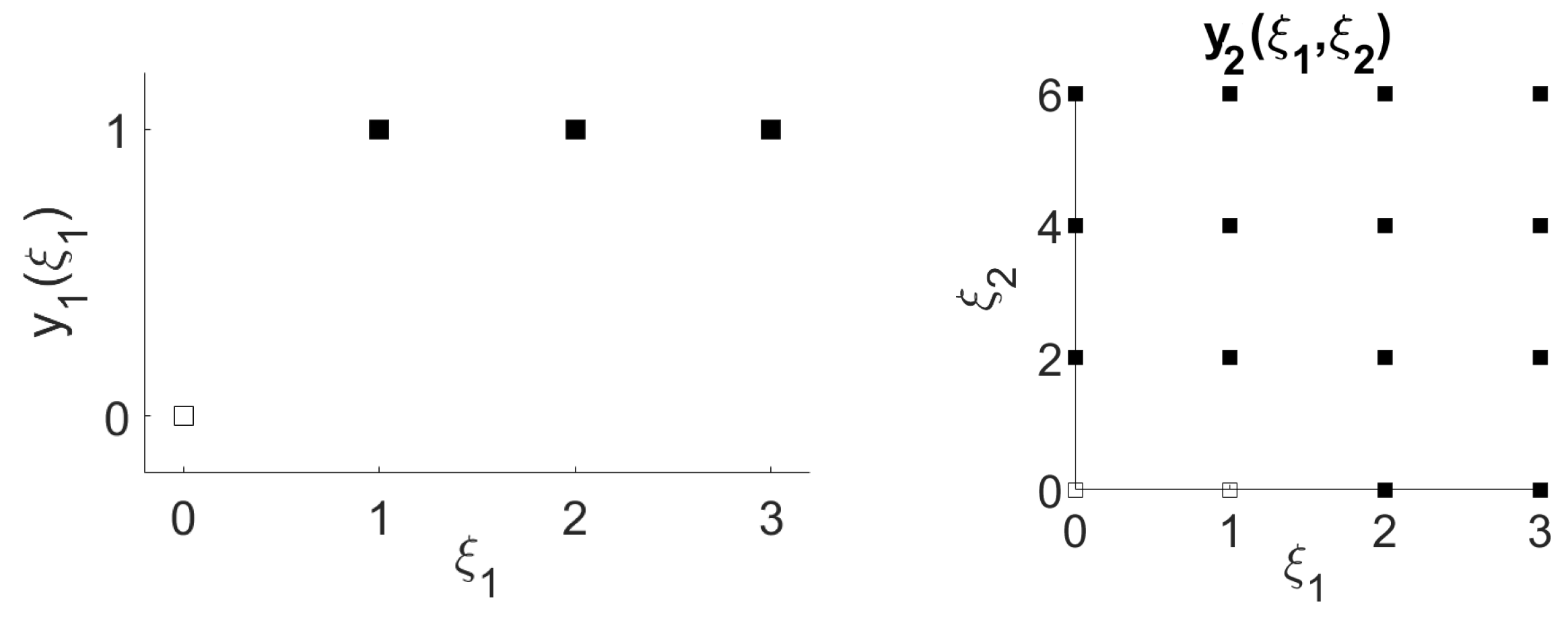
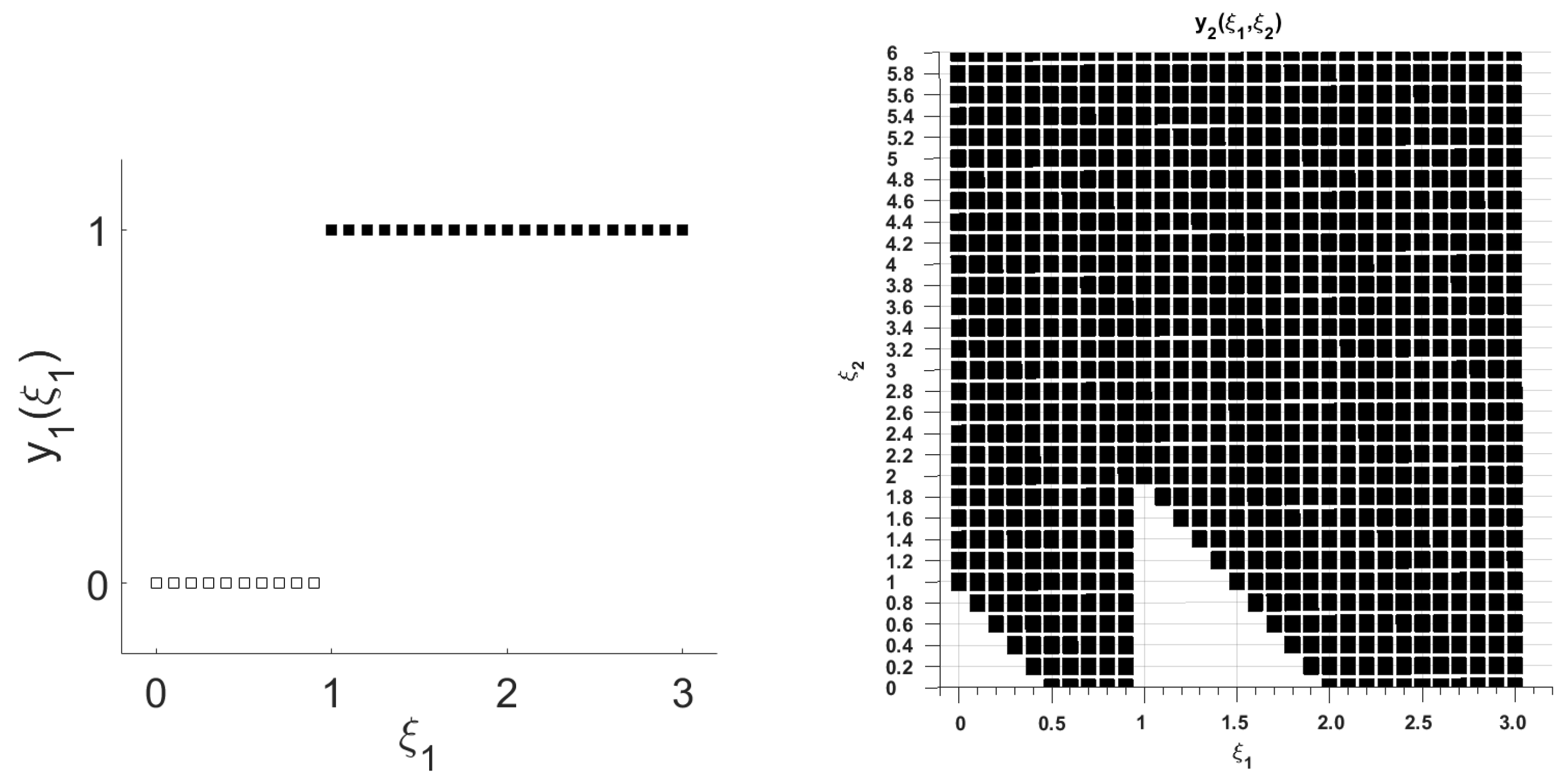
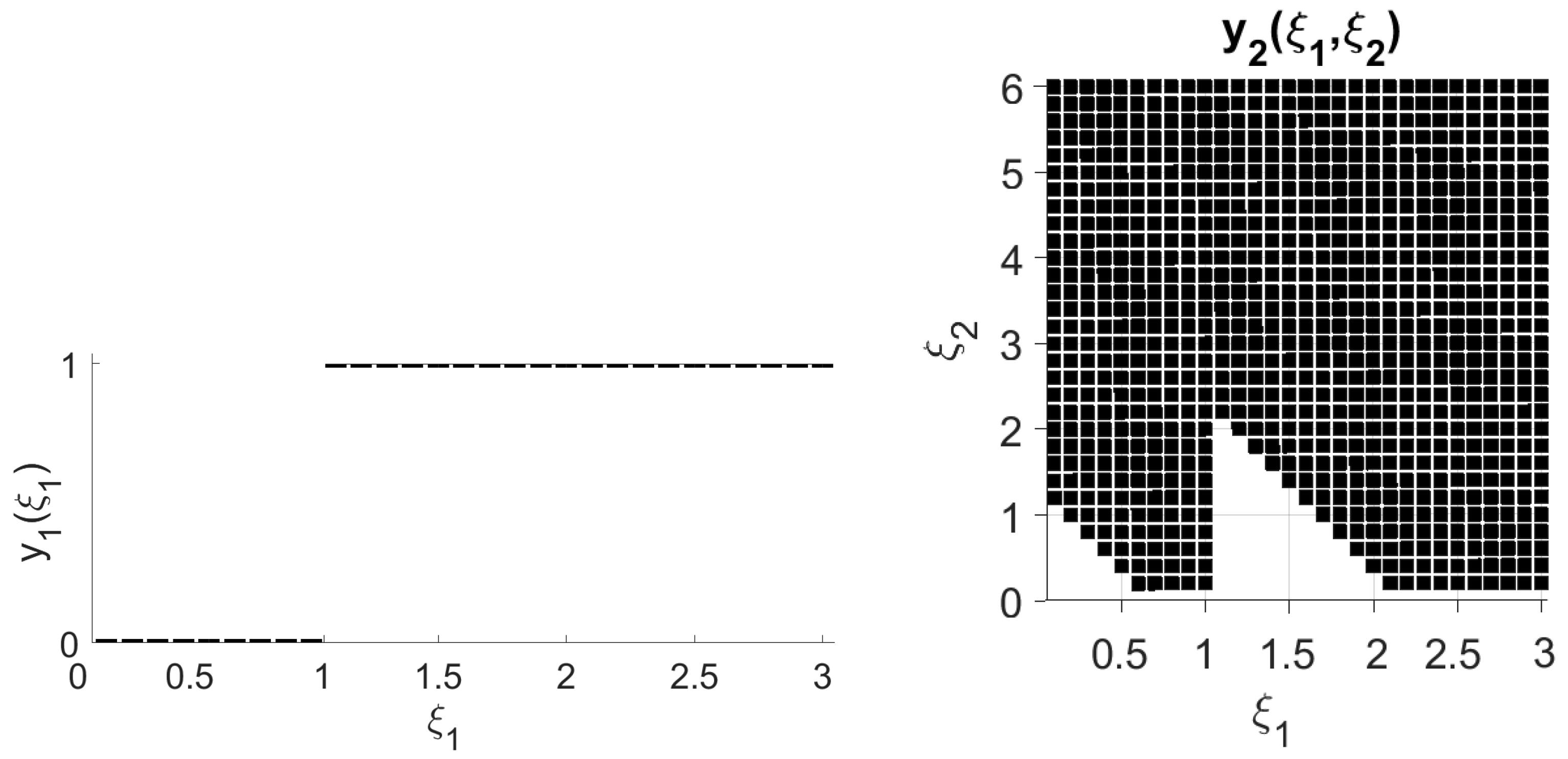
In this work, all the mixed-integer linear optimization problems were modeled in GAMS 25 and solved using CPLEX 12 solver on a workstation (Intel Xeon Dual 20 Core 2.0 GHz Processor, 128 GB DDR4 ECC RAM). Table 1 present the results of the above model for 4, 11, 31 and 99 branches per node. Figure 2 and Figure 3 illustrate the binary solution for 4 and 31 branches per node, respectively. In these figures, the black squares indicate a value of 1 and the white squares indicate a value of 0. Table 1 shows that, by increasing the number of scenarios, the optimal objective value converges to a value around 1.6 . We use this as a benchmark for comparing the different methods to be discussed.
Regarding the recourse decision, Figure 3 illustrates that, for y 1 ( ξ 1 ) , there is a change point around 1 for ξ 1 . For y 2 ( ξ 1 , ξ 2 ) , there are three change points at around 0.5, 1 and 2 for ξ 1 , and two change points at around 1 and 2 for ξ 2 . Those values can be used as a basis for comparison while the lifting and partitioning methods are implemented.

3. Binary Decision Rule with Lifted Uncertainty

3.1. Uncertainty Lifting

Bertsimas and Georghiou [27] proposed a decision rule method for adaptive binary variables. This method enforces a linear relation between the binary variable and the lifted uncertain parameters. In this method, 0–1 indicator functions are defined based on a set of breakpoints for each uncertain parameter. The utilization of the indicator functions results in a nonconvex lifted uncertainty set. To resolve this problem, convex overestimation is applied to the lifted nonconvex set in order to obtain a convex set. The accuracy of the solution can be improved by increasing the number of breakpoints in the lifted set. While traditional scenario-tree methods result in an exponential growth of model size which restricts the application in large-scale problems, the lifting method provides the scalability and tractability required for large-scale problems.
Consider a single uncertain parameter ξ q , t subject to the interval Ξ q , t = { ξ ̲ q , t ξ q , t ξ ¯ q , t } , and assume that the interval is divided into ( r ¯ q , t + 1 ) subintervals using r ¯ q , t breakpoints: α r , q , t , r = 1 , , r ¯ q , t . To lift the uncertainty, the indicator functions Q r , q , t ( · ) of uncertain parameters are used. The following list summarizes the notation used for lifting a single uncertain parameter ξ q , t :
r ¯ q , t scalar, number of breakpoints applied for ξ q , t
α r , q , t scalar, value of the r-th breakpoint for ξ q , t , r = 1 , , r ¯ q , t
as a generalization, we denote the bounds as: α 0 , q , t ξ ̲ q , t , α r ¯ q , t + 1 , q , t ξ ¯ q , t
α 0 , q , t < α 1 , q , t < . . . < α r ¯ q , t , q , t < α r ¯ q , t + 1 , q , t
Q r , q , t the r-th lifted uncertain parameter for ξ q , t (an indicator function of ξ q , t ),
  Q r , q , t ( ξ q , t ) = 1 , if ξ q , t α r , q , t 0 , if ξ q , t < α r , q , t
Q q , t vector of all lifted parameters for ξ q , t : [ Q 1 , q , t , , Q r ¯ q , t , q , t ]
Q t vector of all lifted parameters for ξ t : = [ Q 1 , t , , Q q ¯ t , t ]
Q [ t ] vector, all lifted parameters for ξ [ t ] : [ 1 , Q 1 , . . . , Q t ]
 the first element 1 is used for the intercept term while implementing linear decision rule
ξ q , t vector of overall (original + lifted) uncertainty related to parameter ξ q , t : ξ q , t , Q q , t
ξ t vector of overall uncertainty for stage t: ξ 1 , t , , ξ q ¯ t , t
ξ [ t ] vector of overall uncertainty from stage 1 to t: 1 , ξ 1 , , ξ t
ξ vector of overall uncertainty from stage 1 to T: 1 , ξ 1 , , ξ T
Ξ p , q , t the p-th line segment of the lifted uncertainty set for ξ q , t , p = 1 , , r ¯ q , t + 1
Ξ q , t the lifted uncertainty set (nonconvex) for ξ q , t
Ξ the lifted uncertainty set (nonconvex) for ξ
ν i , p , q , t the two extreme points of Ξ p , q , t , i = 1 , 2
  ν 1 , p , q , t = α p 1 , q , t , 1 , , 1 p 1 times , 0 , , 0 r ¯ q , t p + 1 times , p = 1 , , r ¯ q , t + 1
  ν 2 , p , q , t = α p , q , t , 1 , , 1 p 1 times , 0 , , 0 r ¯ q , t p + 1 times , p = 1 , , r ¯ q , t + 1
η i , p , q , t scalar, coefficient of extreme points in convex full formulation
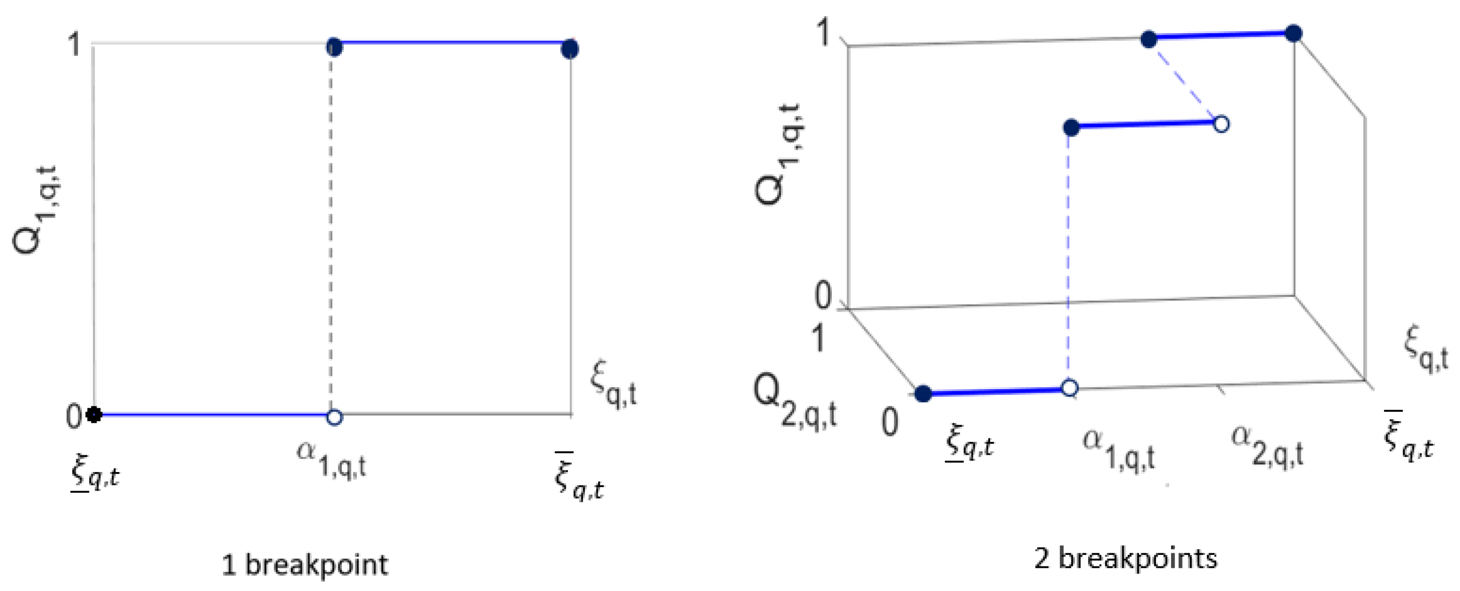
Figure 4 illustrates the lifted uncertainty set ( Ξ q , t ) for a single uncertain parameter ξ q , t based on 1 and 2 breakpoints. It is clear that the lifted uncertainty set is nonconvex since it contains disconnected pieces ( Ξ 1 , q , t , , Ξ R q , t + 1 , q , t ) in a higher dimensional space.
In addition, projection matrices P ξ [ t ] R | ξ [ t ] | × | ξ | and P Q [ t ] R | Q [ t ] | × | ξ | are used in order to obtain ξ [ t ] and Q [ t ] ( ξ ) from the overall uncertainty vector, as follows:
ξ [ t ] = P ξ [ t ] ξ t = 1 , , T
Q [ t ] ( ξ ) = P Q [ t ] ξ t = 1 , , T
Based on the above notation and the original uncertainty set definition in Equation (2), the lifted nonconvex uncertainty set for ξ can be written as:
Ξ = { ξ : P ξ [ T ] ξ Ξ ; ξ q , t Ξ q , t , t = 1 , , T , q = 1 , , q ¯ t }
The nonconvexity of the lifted uncertainty set poses challenges to the optimization problem. The lifted set is convexified such that the semi-infinite constraints can be addressed. Given the 2 ( r ¯ q , t + 1 ) extreme points, the convex hull of Ξ q , t can be constructed as:
c o n v ( Ξ q , t ) = { ξ q , t = [ ξ q , t , Q q , t ] : η i , p , q , t ξ q , t = p = 1 r ¯ q , t + 1 i = 1 2 η i , p , q , t ν i , p , q , t p = 1 r ¯ q , t + 1 i = 1 2 η i , p , q , t = 1 η i , p , q , t > 0 , i = 1 , 2 ; p = 1 , , r ¯ q , t + 1 }
Based on the above convex hull, we define the following convex overestimation for the overall uncertainty set Ξ defined in Equation (6):
Ξ ^ = { ( ξ , η ) : P ξ [ T ] ξ Ξ ; ( ξ q , t , η q , t ) c o n v ( Ξ q , t ) , t = 1 , , T , q = 1 , , q ¯ t }
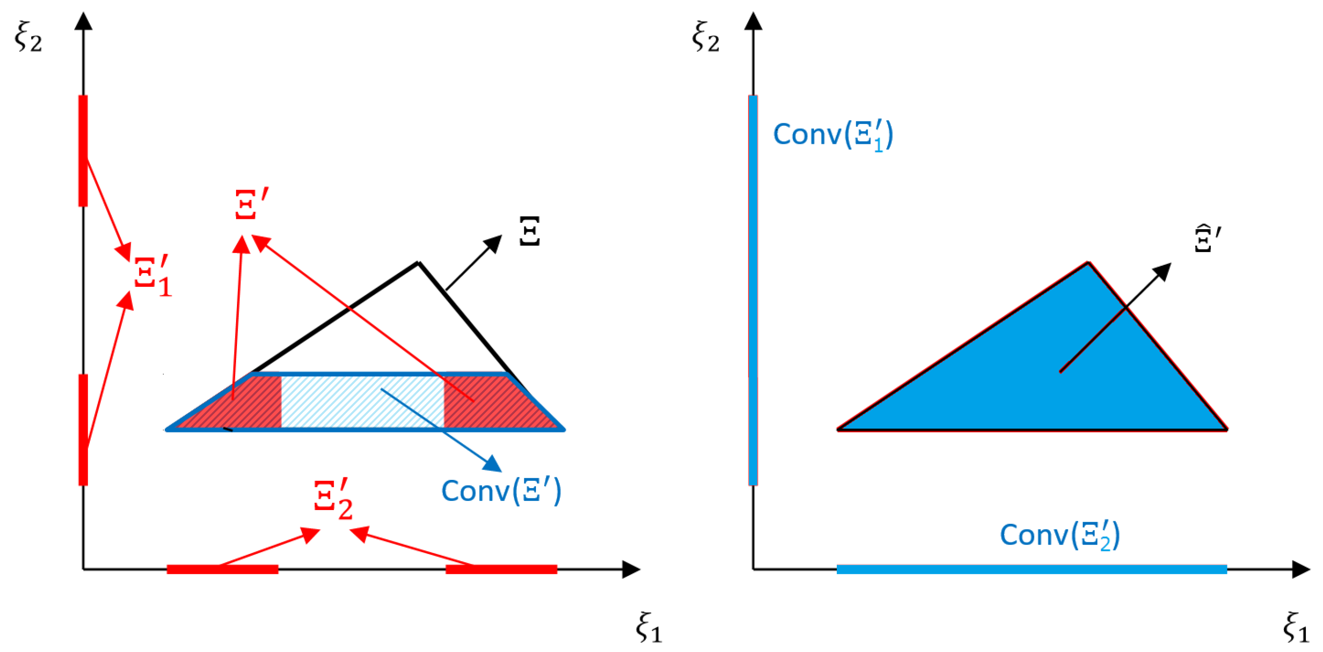
Notice that the convex hull of Ξ , c o n v ( Ξ ) , is a subset of the above overestimation. Figure 5 illustrates the relation between c o n v ( Ξ ) and the overestimation Ξ ^ . The left figure illustrates Ξ according to Equation (6). Ξ is obtained by intersecting the original uncertainty set Ξ (the black triangle) and the nonconvex sets Ξ 1 and Ξ 2 denoted by discontinuous red lines segments. Notice that the sets Ξ 1 and Ξ 2 are at least two dimensional where the dimension depends on the number of breakpoints used in the definition of the lifted set. However, for illustration purposes, the dimension of Ξ 1 and Ξ 2 is assumed to be one since using two dimensions on each axis will make the visualization impossible. The blue shaded area demonstrates c o n v ( Ξ ) . In the right figure, the blue triangle corresponds to the overestimation set Ξ ^ (Equation (8)), which is obtained by intersecting the original uncertainty set Ξ and c o n v ( Ξ 1 ) × c o n v ( Ξ 2 ) . As the figure shows, Ξ ^ is an overestimation of c o n v ( Ξ ) .
Finally, for simplicity in derivation, we project the polyhedral uncertainty set Ξ ^ onto the space of ξ , and compactly write it as:
Ξ ^ = { ξ : J ξ h }
where J and h are constant matrix calculated from the breakpoints value and the original uncertainty set parameters J , h .
Illustrating example (cont.)
In this section, the lifting method is applied to the illustrating example. Two breakpoints are considered for each uncertain parameter (r = 1, 2):
for ξ 1 : α 1 , 1 , 1 = 1 , α 2 , 1 , 1 = 2 for ξ 2 : α 1 , 1 , 2 = 2 , α 2 , 1 , 2 = 4
The lifted uncertainty vector is formulated as:
ξ = 1 , ξ 1 , Q 1 , 1 , 1 ( ξ 1 ) , Q 2 , 1 , 1 ( ξ 1 ) , ξ 2 , Q 1 , 1 , 2 ( ξ 2 ) , Q 2 , 1 , 2 ( ξ 2 )
The 0–1 indicator functions are defined as:
Q 1 , 1 , 1 ( ξ 1 ) = 1 , if ξ 1 1 0 , if ξ 1 < 1 , Q 2 , 1 , 1 ( ξ 1 ) = 1 , if ξ 1 2 0 , if ξ 1 < 2 Q 1 , 1 , 2 ( ξ 2 ) = 1 , if ξ 2 2 0 , if ξ 2 < 2 , Q 2 , 1 , 2 ( ξ 2 ) = 1 , if ξ 2 4 0 , if ξ 2 < 4
The associated projection matrices and the corresponding (original or lifted) uncertainty vectors are:
P ξ [ 1 ] = 1 0 0 0 0 0 0 0 1 0 0 0 0 0 , ξ [ 1 ] = P ξ [ 1 ] ξ = [ 1 , ξ 1 ] P ξ [ 2 ] = 1 0 0 0 0 0 0 0 1 0 0 0 0 0 0 0 0 0 1 0 0 , ξ [ 2 ] = P ξ [ 2 ] ξ = [ 1 , ξ 1 , ξ 2 ] P Q [ 1 ] = 1 0 0 0 0 0 0 0 0 1 0 0 0 0 0 0 0 1 0 0 0 , Q [ 1 ] ( ξ ) = P Q [ 1 ] ξ = [ 1 , Q 1 , 1 , 1 , Q 2 , 1 , 1 ] P Q [ 2 ] = 1 0 0 0 0 0 0 0 0 1 0 0 0 0 0 0 0 1 0 0 0 0 0 0 0 0 1 0 0 0 0 0 0 0 1 , Q [ 2 ] ( ξ ) = P Q [ 2 ] ξ = [ 1 , Q 1 , 1 , 1 , Q 2 , 1 , 1 , Q 1 , 1 , 2 , Q 2 , 1 , 2 ]
The lifted uncertainty set is defined as: Ξ = { ξ R 2 : P ξ [ 2 ] ξ Ξ , ξ q , t Ξ q , t } , where Ξ = { ξ : ξ 1 [ 0 , 3 ] , ξ 2 [ 0 , 6 ] } . Next, the convex hull for each single lifted uncertain parameter c o n v ( Ξ q , t ) is constructed. For simplicity in presentation, η i , p , 1 , 1 and η i , p , 1 , 2 are represented by η p , i and η p , i in the following equations, respectively.
c o n v ( Ξ 1 , 1 ) = ξ 1 , 1 : η 1 , 1 , η 1 , 2 , η 2 , 1 , η 2 , 2 , η 3 , 1 , η 3 , 2 0 , η 1 , 1 + η 1 , 2 + η 2 , 1 + η 2 , 2 + η 3 , 1 + η 3 , 2 = 1 ξ 1 Q 1 , 1 , 1 Q 2 , 1 , 1 = η 1 , 1 0 0 0 + η 1 , 2 α 1 , 1 , 1 0 0 + η 2 , 1 α 1 , 1 , 1 1 0 + η 2 , 2 α 2 , 1 , 1 1 0 + η 3 , 1 α 2 , 1 , 1 1 1 + η 3 , 2 3 1 1 c o n v ( Ξ 1 , 2 ) = ξ 1 , 2 : η 1 , 1 , η 1 , 2 , η 2 , 1 , η 2 , 2 , η 3 , 1 , η 3 , 2 0 , η 1 , 1 + η 1 , 2 + η 2 , 1 + η 2 , 2 + η 3 , 1 + η 3 , 2 = 1 ξ 2 Q 1 , 1 , 2 Q 2 , 1 , 2 = η 1 , 1 0 0 0 + η 1 , 2 α 1 , 1 , 2 0 0 + η 2 , 1 α 1 , 1 , 2 1 0 + η 2 , 2 α 2 , 1 , 2 1 0 + η 3 , 1 α 2 , 1 , 2 1 1 + η 3 , 2 6 1 1
The overall convex hull c o n v ( Ξ ) is a subset of the following overestimated set Ξ ^ = { ξ R 2 : P ξ [ 2 ] ξ Ξ , ξ q , t c o n v ( Ξ q , t ) , q = 1 , t = 1 , 2 } .

3.2. Binary Decision Rule

To approximate the optimal adaptive binary solution, binary decision rule is employed. It enforces a linear relation with respect to the lifted uncertainty (indicator function). The binary decision y t depends on uncertainty up to time stage t. In binary decision rule, y t is approximated by a linear combination of indicator functions from stage 1 to stage t, Q [ t ] ( ξ ) :
y t ( ξ [ t ] ) = Y t Q [ t ] ( ξ ) t = 1 , , T
where the coefficients only take the following possible integer values: Y t { 1 , 0 , 1 } | y t | × | Q [ t ] | . Furthermore, binary restriction on original variables need to be enforced, hence:
0 Y t Q [ t ] ( ξ ) e ξ Ξ , t = 1 , , T
where e is the vector of all ones. By applying the binary decision rule to the general stochastic formulation, a semi-infinite optimization problem with a finite number of variables but infinite number of constraints is obtained:
min E ξ t ( D t ξ [ t ] ) Y t Q [ t ] ( ξ )
s . t . τ = 1 t B t , τ Y τ Q [ τ ] ( ξ ) E t ξ [ t ] ξ Ξ , t = 1 , , T
0 Y t Q [ t ] ( ξ ) e ξ Ξ , t = 1 , , T
In the above model, the constraints contain a nonconvex indicator functions of original uncertain parameters. Using Equations (5a) and (5b), the stochastic model can be written as the following model with linear constraints with respect to the lifted uncertainty ξ :
min E ξ t ( D t P ξ [ t ] ξ ) Y t P Q [ t ] ξ
s . t . τ = 1 t B t , τ Y τ P Q [ τ ] ξ E t P ξ [ t ] ξ ξ Ξ , t 1 , , T
0 Y t P Q [ t ] ξ e ξ Ξ , t 1 , , T
Since the lifted uncertainty set Ξ is nonconvex and consequently the problem is still intractable. The problem can be conservatively approximated by using the convex overestimation Ξ ^ of the lifted uncertainty set as defined in Equation (9).
min E ξ t ( D t P ξ [ t ] ξ ) Y t P Q [ t ] ξ
s . t . τ = 1 t B t , τ Y τ P Q [ τ ] ξ E t P ξ [ t ] ξ ξ Ξ ^ , t 1 , , T
0 Y t P Q [ t ] ξ e ξ Ξ ^ , t 1 , , T
Since constraints (14b) and (14c) are linear with respect to ξ , and the uncertainty set Ξ ^ is a polyhedral set, duality theorem can be used to covert this semi-infinite problem into its deterministic robust counterpart. As an example, constraint (14b) can be written as
τ = 1 t B t , τ Y τ P Q [ τ ] E t P ξ [ t ] ξ 0 ξ Ξ ^ , t 1 , , T
or equivalently as in the following, based on the uncertainty set definition in Equation (9)
max J ξ h τ = 1 t B t , τ Y τ P Q [ τ ] E t P ξ [ t ] ξ 0 t 1 , , T
Its deterministic counterpart is obtained as follows after applying duality to the inner maximization problem:
h θ t 0 t J θ t = ( τ = 1 t B t , τ Y τ P Q [ τ ] E t P ξ [ t ] ) t θ t 0 t
Similarly, constraint (14c) can be divided into two parts: 0 Y t P Q [ t ] ξ and Y t P Q [ t ] ξ e , and the robust counterpart is derived accordingly. The overall deterministic counterpart formulation is given by
min t Tr ( E [ ξ ξ ] P ξ [ t ] D t Y t P Q [ t ] )
s . t . h θ t 0 t
J θ t = ( τ = 1 t B t , τ Y τ P Q [ τ ] E t P ξ [ t ] ) t
θ t 0 t
h λ t 0 t
J λ t = ( Y t P Q [ t ] ) t
λ t 0 t
h ϕ t e t
J ϕ t = ( Y t P Q [ t ] ) t
ϕ t 0 t
Y t { 1 , 0 , 1 } | y t | × | Q [ t ] |
where Tr ( · ) is trace operator and E [ ξ ξ ] can be derived from the know distribution of the uncertainty.
Illustrating example (cont.)
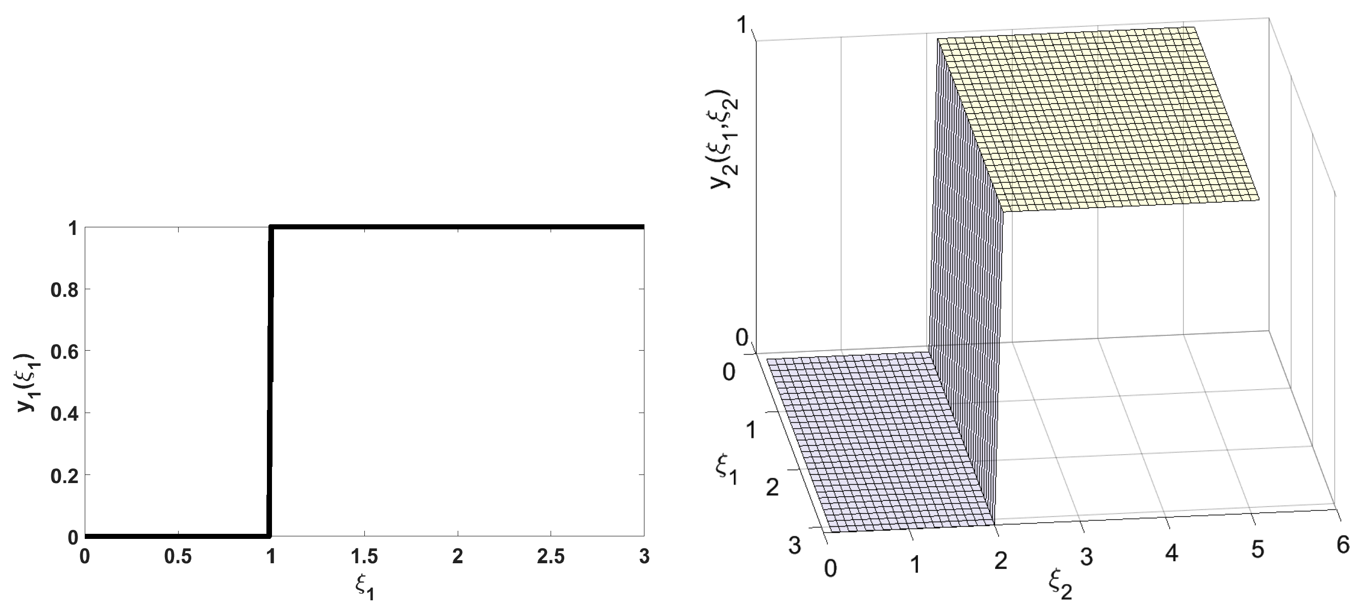
Table 2 presents the results of the above lifting method for different numbers of breakpoints. For 1 breakpoint case, the breakpoint values are set as 1.5 for ξ 1 , and 3 for ξ 2 . For 2 breakpoints case, the breakpoint values are set as ( 1 , 2 ) for ξ 1 , and ( 2 , 4 ) for ξ 2 . For 9 breakpoints case, the breakpoint values are set as ( 0.3 , 0.6 , 0.9 , , 2.7 ) for ξ 1 , and ( 0.6 , 1.2 , , 5.4 ) for ξ 2 . The objective did not improve beyond 1.333 even for nine breakpoints. This observation indicates that the lifting solution quality may be restricted. Using the definition of the lifting method for the binary variable, we can plot the y 1 ( ξ 1 ) and y 2 ( ξ 1 , ξ 2 ) variables. For the case of 2 breakpoints, the model solution is Y 1 = [ 0 , 1 , 0 ] and Y 2 = [ 0 , 0 , 0 , 1 , 0 ] , and the adaptive binary variables are expressed as:
y 1 ( ξ 1 ) = Y 1 Q [ 1 ] = [ 0 , 1 , 0 ] × [ 1 , Q 1 , 1 , 1 ( ξ 1 ) , Q 2 , 1 , 1 ( ξ 1 ) ] = Q 1 , 1 , 1 ( ξ 1 ) y 2 ( ξ 1 , ξ 2 ) = Y 2 Q [ 2 ] = [ 0 , 0 , 0 , 1 , 0 ] × [ 1 , Q 2 , 1 , 1 ( ξ 1 ) , Q 1 , 1 , 2 ( ξ 2 ) , Q 2 , 1 , 2 ( ξ 2 ) ] = Q 1 , 1 , 2 ( ξ 2 )
As shown in Figure 6, the binary variable y 2 is only a function of parameter ξ 2 which indicates a restricted solution quality.

3.3. Breakpoint Optimization for Lifting Method

In this section, we assume that the location of breakpoints is not pre-fixed and they are optimized instead. Based on Equation (9), the breakpoints information is contained in the parameters J , h and can be formulated as:
J = J 0 + J 1 α h = h 0 + h 1 α
where J 0 , J 1 , h 0 , h 1 are known constant matrices/vectors, α is the vector involving all location information of breakpoints. The above formulated J and h should be substituted in the dual counterpart formulation (Equations (15a)–(15j)) to complete the variable breakpoint lifting technique.
min E ξ t Tr ( E [ ξ ξ ] P ξ [ t ] D t Y t P Q [ t ] )
s . t . ( h 0 + h 1 α ) θ t 0 t
( J 0 + J 1 α ) θ t = ( s = 1 t B ts Y s P Q [ s ] E t P ξ [ t ] ) t
θ t 0 t
( h 0 + h 1 α ) λ t 0 t
( J 0 + J 1 α ) λ t = ( Y t P Q [ t ] ) t
λ t 0 t
( h 0 + h 1 α ) ϕ t e t
( J 0 + J 1 α ) ϕ t = ( Y t P Q [ t ] ) t
ϕ t 0 t
Y t { 1 , 0 , 1 } | y t | × | Q [ t ] |
Notice that the expectation of the lifted uncertainty E ( ξ ) also depends on the location of the variable breakpoints, so E [ ξ ξ ] is also a function of α (which can be analytically evaluated based on the distribution information). The resulting model will be a mixed integer nonlinear optimization problem, where the integer variables are the binary decision rule coefficients Y t , and the continuous variables include the dual variables θ , λ , ϕ and the breakpoint locations α .
In this work, all MINLP problems were solved using the ANTIGONE 1.0 solver [30] in the GAMS 25 platform on a workstation (Intel Xeon Dual 20 Core 2.0 GHz Processor, 128 GB DDR4 ECC RAM) using a time resource limit of 10 h. The reported solution have zero optimality gap, otherwise it is reported. Using a single variable breakpoint in the illustrating example, the obtained objective ( 1.333 ) is better than using a single fixed breakpoint ( 1.000 ). This shows the advantage of variable breakpoint lifting compared to the fixed breakpoint method. However, in this example, using more than one variable breakpoint did not further improve the objective, as shown in Table 3. This observation shows that the lifting method’s solution quality is restricted.
The optimized breakpoint values are summarized below:
  • For 1 breakpoint case, 1 for ξ 1 , 2 for ξ 2
  • For 2 breakpoints case, (0, 1) for ξ 1 , (0, 2) for ξ 2
  • For 9 breakpoints case, (1.5, 1.5, 1.5, 1.5, 1.5, 1.5, 3, 3, 3) for ξ 1 , (1, 1, 1, 1, 2.52, 3.6, 4.2, 4.8, 5.4) for ξ 2
Notice that the variable breakpoints are not forced to be different to each other, so the solution has overlapped breakpoints while the number of breakpoints increases.

4. Finite Adaptability with Uncertainty Set Partitioning

4.1. Uncertainty Set Partitioning

In this method, the uncertainty set is divided into small partitions and a constant binary decision is assumed for each partition. Similarly to the lifting method, we define breakpoints for each uncertain parameter and each subset is a box type of uncertainty set. Figure 7 illustrates the partitioning of a two-dimensional rectangular uncertainty set and the corresponding scenario tree with each branch representing a subinterval for each parameter. In this figure, the interval of each uncertain parameter is divided into three segments such that there are three nodes in the first stage and nine nodes in the second stage. The following notations were used in this method:
s:
a scenario (each scenario is represented by a matrix structure (allowing empty elements), its element s q , t gives the subinterval index of the uncertain parameter ξ q , t ) under this scenario
r ¯ q , t :
scalar, number of breakpoints for ξ q , t
α s q , t , q , t :
scalar, upper bound value for element ξ q , t under scenario s
As an example, consider a two-stage problem: the first stage has uncertain parameters ξ 1 , 1 , ξ 2 , 1 and the second stage has one uncertain parameter ξ 1 , 2 . Assume no breakpoint is applied to ξ 1 , 1 , one breakpoint is applied to ξ 2 , 1 , and two breakpoints are applied to ξ 1 , 2 . Then, the set S is:
s S = 1 1 1 , 1 1 2 , 1 2 1 , 1 2 2 , 1 3 1 , 1 3 2
where “*” denotes that the corresponding element does not exist.
For each scenario s S , the uncertainty set is a hyper-rectangular (subset of original set Ξ )
Ξ s = { ξ : α s q , t 1 , q , t ξ q , t α s q , t , q , t ; t = 1 , , T , q = 1 , , q ¯ t }
which can be compactly written as
Ξ s = { ξ : W s ξ V s }

4.2. Finite Adaptability

Next, the finite adaptability method (also denoted as “partitioning method” in this work) is applied to the original problem (1a)–(1c). The idea is a combination of scenario tree-based stochastic formulation and robust optimization. For each scenario, we enforce constraint satisfaction over a uncertainty set as defined in Equation (17) instead of a single point in the uncertainty space. The resulting model can be cast as:
min y s S p s t = 1 T D t E Ξ s ( ξ ) y t , s
s . t . τ = 1 t A t τ y τ , s E t ξ t , s , ξ Ξ s
y t , s = y t , s ( t , s , s ) S P
where the last constraint is enforcing non-anticipativity and S P is the set of all scenarios with the same path up to time t:
S P = { ( t , s , s ) : s q , τ = s q , τ , τ = 1 , , t , q = 1 , , q ¯ τ }
Reformulating the semi-infinite constraint using linear programming duality, the corresponding robust scenario-based formulation is
min y s S p s t = 1 T D t E Ξ s ( ξ ) y t , s
s . t . V s θ t , s τ t A t τ y τ , s s , t
W s θ t , s = E t s , t
θ t , s 0 s , t
y t , s = y t , s ( t , s , s ) S P
Illustrating example (cont.)
In this section, the partitioning method is applied to the illustrating example (3a)–(3d) and the results are presented. Figure 7 illustrates the partitioning and the corresponding scenario tree for the illustrating example.
The formulation for the partitioning of the uncertainty set is based on two equally-spaced breakpoints for each uncertainty element: for ξ 1 , 1 [ 0 , 3 ] , the breakpoints are set as 0 < 1 < 2 < 3 ; for ξ 1 , 2 [ 0 , 6 ] the breakpoints are 0 < 2 < 4 < 6 . Hence, S = [ 1 , 1 ] , [ 1 , 2 ] , [ 1 , 3 ] , [ 2 , 1 ] , [ 2 , 2 ] , [ 2 , 3 ] , [ 3 , 1 ] , [ 3 , 2 ] , [ 3 , 3 ] .
The non-anticipativity condition set S P contains the following elements:
1 , [ 1 , 1 ] , [ 1 , 2 ] , 1 , [ 1 , 1 ] , [ 1 , 3 ] , 1 , [ 1 , 2 ] , [ 1 , 3 ] 1 , [ 2 , 1 ] , [ 2 , 2 ] , 1 , [ 2 , 1 ] , [ 2 , 3 ] , 1 , [ 2 , 2 ] , [ 2 , 3 ] 1 , [ 3 , 1 ] , [ 3 , 2 ] , 1 , [ 3 , 1 ] , [ 3 , 3 ] , 1 , [ 3 , 2 ] , [ 3 , 3 ]
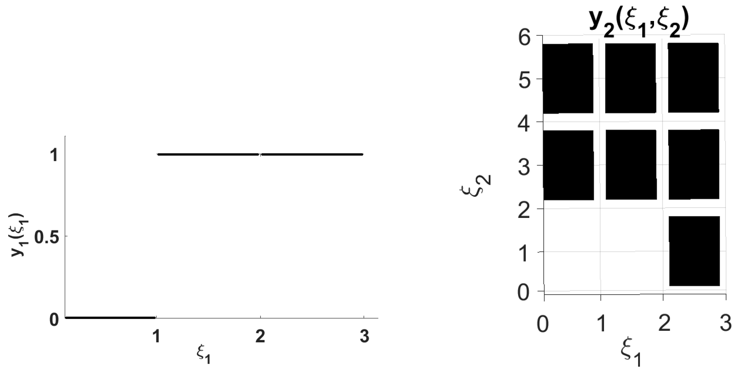
The partitioning-based model is the MILP problem. Table 4 presents the results from the finite adaptability method. As the number of partitions increases, the objective improves until it reaches close to the optimal solution obtained from scenario method (−1.594 for 99 branches per node). For comparison, the branches and breakpoints are evenly distributed in the scenario and finite adaptability method, respectively. For 29 breakpoints in the partitioning method and 31 branches in the scenario method, the optimal objectives are −1.589 and −1.605, respectively. Figure 8 and Figure 9 illustrate the partitioning solutions for 2 and 29 breakpoints. As the figures demonstrates, there is a close match between the partitioning and scenario solution.

4.3. Breakpoint Optimization in Partitioning Method

In the variable breakpoint partitioning technique, the location of breakpoints is unknown a priori and it is optimized instead. The location of breakpoints is reflected in the V s matrix of Equation (17) and it is formulated as follows:
V s = V s 0 + V s 1 α s S
where V s 0 and V s 1 are constant matrices. The corresponding robust scenario-based formulation is
min y s S p s t = 1 T D t E Ξ s ( ξ ) y t , s
s . t . ( V s 0 + V s 1 α ) θ t , s τ = 1 t A t τ y τ , s s , t
W s θ t , s = E t s , t
θ t , s 0 s , t
y t , s = y t , s ( t , s , s ) S P
In this formulation, the probability of the occurrence of each scenario depends on the location of breakpoints since the length of each dimension in each scenario depends on the location of breakpoints. The probability p s for each scenario and E Ξ s ( ξ ) are both functions of α and they can be evaluated based on the distribution of the uncertainty.
Table 5 summarized the results of the variable partitioning technique. It can be observed that, for the same number of partitions, the variable partitioning method provided a better objective compared to the fixed breakpoint method. For instance, for 2 breakpoints per uncertain parameter, the variable and fixed methods’ objectives are −1.500 and −1.444, respectively. The variable method even provided a better objective with just three breakpoints compared to the fixed method with nine breakpoints. However, for a large number of partitions, the fixed breakpoint method is much faster in terms of solution and it could provide a better objective using 29 breakpoints in less than 1 s compared to the variable method using 5 breakpoints after about 18 min run time.

4.4. Flexibility Comparison

We can observe from Table 2 that, for the illustrating problem, the lifting method’s objective does not improve beyond −1.333, even for nine breakpoints, while the partitioning method could provide a better objective of −1.444 with two breakpoints for each parameter. In this section, we investigate the reason why lifting method leads to restricted solution quality compared to the partitioning method. For this purpose, the solution from partitioning method is substituted into the decision rule solution from the lifting method. Note that the same breakpoints are applied in the lifting and partitioning method (as shown in Figure 7). This will result in a linear system of equations. If the set of equations has no solution, this means that the lifting method has a restricted flexibility such that it cannot cover the solution of the partitioning method.
Figure 8 presents the partitioning solution. In this problem, the intervals for ξ 1 , ξ 2 are divided into three equally distributed pieces. Based on the binary decision rule equations:
y t = Y t Q [ t ] Q [ 1 ] = [ 1 , Q 1 , 1 , 1 , Q 2 , 1 , 1 ] Q [ 2 ] = [ 1 , Q 1 , 1 , 1 , Q 2 , 1 , 1 , Q 1 , 1 , 2 , Q 2 , 1 , 2 ]
For the three nodes at stage 1, the corresponding lifted uncertainty vector Q [ 1 ] takes the three following values:
Node 1 : Y 1 [ 1 , 0 , 0 ] = 0 Node 2 : Y 1 [ 1 , 1 , 0 ] = 1 Node 3 : Y 1 [ 1 , 1 , 1 ] = 1
There is a solution Y 1 = [ 0 , 1 , 0 ] for the above equations. For the nine nodes at stage 2, the lifted uncertainty vector takes nine different values for nodes 4 to 12:
Node 4 : Y 2 [ 1 , 0 , 0 , 0 , 0 ] = 0 Node 5 : Y 2 [ 1 , 0 , 0 , 1 , 0 ] = 1 Node 6 : Y 2 [ 1 , 0 , 0 , 1 , 1 ] = 1 Node 7 : Y 2 [ 1 , 1 , 0 , 0 , 0 ] = 0 Node 8 : Y 2 [ 1 , 1 , 0 , 1 , 0 ] = 1 Node 9 : Y 2 [ 1 , 1 , 0 , 1 , 1 ] = 1 Node 10 : Y 2 [ 1 , 1 , 1 , 0 , 0 ] = 1 Node 11 : Y 2 [ 1 , 1 , 1 , 1 , 0 ] = 1 Node 12 : Y 2 [ 1 , 1 , 1 , 1 , 1 ] = 1
There is no solution Y 2 satisfying this linear system of equations (there are nine equations and five variables for Y 2 ). This evidence indicates that lifting the method’s solution is restricted compared to the partitioning method. The limited solution flexibility is due to the affine decision rule over the lifted uncertainty.

5. Case Study: Inventory Control Problem

In this section, an inventory control problem with discrete ordering decisions is studied where the problem is adapted from [27]. This problem can be formulated as an multistage adaptive robust optimization problem with fixed recourse and can be explained as follows. At the beginning of each time period t T = { 1 , , T } , the product demand ξ t is observed. This demand can be satisfied in two ways: (1) by pre-ordering at period t using maximum N lots (binary variable z n , t is introduced to express whether we order from n lots in time period t or not), each delivering a fixed quantity q z at the beginning of period t for a unit cost of c z ; (2) by placing a recourse order during the period t using maximum N lots (binary variable y n , t is introduced for this decision), each delivering immediately a fixed quantity q y for a unit cost of c y . The pre-ordering cost is always less than the immediate ordering cost ( c z < c y ). If the ordered quantity is greater than the demand, the excess units are stored in a warehouse that incurs a unit holding cost of c h and can be used to satisfy future demand. Furthermore, the cumulative volume of pre-orders τ = 1 t n = 1 N q z z n , τ cannot exceed the ordering budget B ¯ t . The objective is to minimize the total ordering and holding costs over the planning horizon by determining the optimal decision of z n , t and y n , t ( ξ [ t ] ) . Equations (21a)–(21e) express the problem formulation.
min E ξ t = 1 T n = 1 N c z q z z n , t + c y q y y n , t ( ξ [ t ] ) + c h I t ( ξ [ t ] )
s . t . I t ( ξ [ t ] ) = I 0 + τ = 1 t n = 1 N q z z n , τ + q y y n , τ ( ξ [ τ ] ) ξ τ t T , ξ Ξ
I t ( ξ [ t ] ) 0 t T , ξ Ξ
τ = 1 t n = 1 N q z z n , τ B ¯ t t T
z n , t { 0 , 1 } , y n , t ( ξ [ t ] ) { 0 , 1 } n , t
Notice that z n , t is a static binary decision variable, while y n , t is the adaptive binary decision variable dependent on the realized uncertainty ξ [ t ] . The uncertainty set is represented as: Ξ = { ξ R T : l ξ u } . Uniform distribution is assumed for all of them. The bounds for each random parameter are chosen from l t [ 0 , 5 ] and u t [ 10 , 15 ] for t = 1 , , T . The cumulative ordering budget equals to B ¯ t = 10 t for t = 1 , T . It is also assumed that q z = q y = 15 / N and the initial inventory is zero ( I 0 = 0 ) .
Two different configurations of the inventory problem are studied in this work (Table 6). In the second configuration, the unit cost for immediate ordering ( c y ), unit cost for storage at warehouse ( c h ) and the maximum number of delivery lots (N) are greater than the first configuration. Since, at the second configuration, the costs for immediate ordering and warehouse are higher, it is therefore more economical to satisfy demand using first-stage decisions. Lifting and partitioning methods using both fixed and variable breakpoints are applied to the case study and the obtained results are discussed.
First, the comparison is made between lifting and partitioning methods using same fixed breakpoint setting. The following results are obtained:
  • The number of variables grows exponentially in the partitioning method while it grows linearly in the lifting. For a large number of time stages (T) and number of breakpoints used ( B r ), the number of variables in the partitioning method can be prohibitively large and it may not be possible to run the model (Table 7 and Table 8). Therefore, considering time and computational resource limitations, the lifting method is suggested for large models (experiments next to T = 10 , B r = 2 in this case study, Table 9 and Table 10). Thus, the ability to run large models can be considered the main advantage of the lifting method.
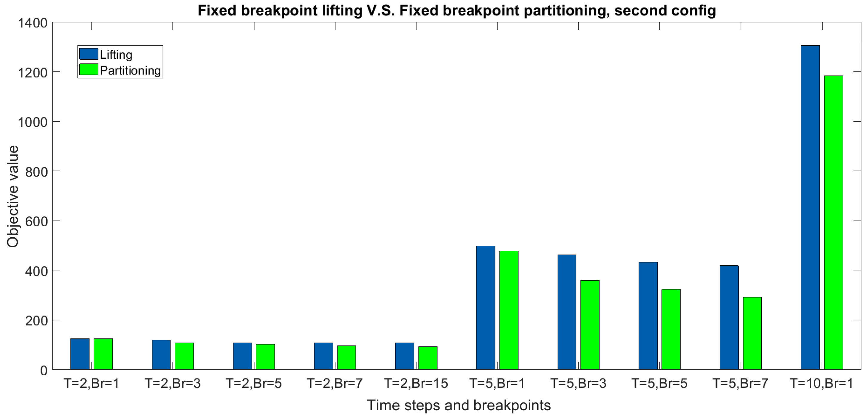
  • It is observed that for experiments with small and medium model size (up to T = 10 , B r = 1 in this case study), the partitioning method provides a better objective value in a shorter run time compared to the lifting method. For instance, for experiments with 5 time steps, the partitioning method provides a better solution in 9.5 s (Table 7, T = 5 , B r = 2 ) compared to the lifting method in 10 h run time (Table 9, T = 5 , B r = 15 ). Figure 10 and Figure 11 compare the fixed breakpoint lifting and finite adaptability (partitioning) methods for the first and second configurations, respectively.
  • In general, in both partitioning and lifting methods, the objective improves by increasing the number of breakpoints except for large problems where the optimality gap is still quite large after 10 h run time limitation (Table 9 and Table 10). Thus, for large models, in order to obtain the best objective in limited run time, there is no need to consider a large number of breakpoints.
Next, the comparison is made between fixed and variable breakpoint methods. The following observations are made:
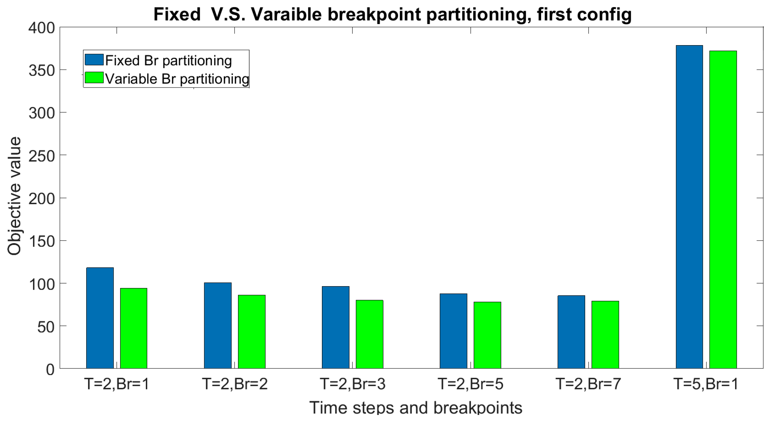
  • Variable breakpoint lifting and partitioning techniques introduce additional variables and require the mixed integer nonlinear optimization compared to mixed integer linear optimization for fixed breakpoint case. As shown in Table 7, Table 9, Table 11 and Table 12, and Figure 12 and Figure 13, the variable breakpoint techniques can provide a better objective compared to fixed methods for small-to-medium size models ( T = 2 and T = 5 ). However, the run time is longer. For a large number of time steps and breakpoints, the problem size is too large such that it is impossible to run the model under computational resource restrictions.
  • For small-to-medium size experiments ( T = 2 , T = 5 ), the fixed breakpoints partitioning method is recommended since it provides the best objective within the shortest run time considering computational resource restrictions.
  • For large-size problems ( T = 10 , T = 20 ), the lifting method under fixed breakpoints is the only method that results in a feasible solution considering the computational resource limitations. The partitioning technique leads to large-size problems such that the solver could not find a solution in the 10 h time limit.

6. Conclusions

In this work, the lifting and partitioning methods for multistage adaptive robust binary optimization problems were studied. Different formulations based on fixed or variable breakpoints setting for each method were presented. Computational studies were made to compare the computational performance and the solution quality. The following conclusions can be made from this study. First, the binary decision rule (lifting)-based method and the finite adaptability (partitioning)-based method share a similar idea of uncertainty set splitting using breakpoints for each uncertain parameter. While the lifting-based method has less solution flexibility than the partitioning method (under the same breakpoint setting), the lifting method has the advantage of superior computational tractability and scalability for large problems. While computational resource restrictions is a major concern (especially for problems with a large number of stages), the lifting method with fixed breakpoints is suggested and the number of breakpoints can be moderately large to avoid inferior solution quality. Otherwise, the partitioning method is suggested. Variable breakpoints can be implemented for partitioning method especially for small number of stages with the usage of small number of breakpoints. As a future research direction, the number of breakpoints can be optimized to avoid unnecessary model complexity.

Author Contributions

Methodology, F.M.N. and Z.L.; Software, F.M.N.; Validation, F.M.N.; Writing—original draft, F.M.N.; Writing—review & editing, Z.L.; Supervision, Z.L.; Funding acquisition, Z.L. All authors have read and agreed to the published version of the manuscript.

Funding

This research received no external funding.

Data Availability Statement

Data is contained within the article.

Acknowledgments

The authors gratefully acknowledge the financial support from the Natural Sciences and Engineering Research Council of Canada (NSERC).

Conflicts of Interest

The authors declare no conflict of interest.

References

  1. Goulart, P.J.; Kerrigan, E.C.; Maciejowski, J.M. Optimization over state feedback policies for robust control with constraints. Automatica 2006, 42, 523–533. [Google Scholar] [CrossRef]
  2. Skaf, J.; Boyd, S.P. Design of affine controllers via convex optimization. IEEE Trans. Autom. Control 2010, 55, 2476–2487. [Google Scholar] [CrossRef]
  3. Aharon, B.T.; Boaz, G.; Shimrit, S. Robust multi-echelon multi-period inventory control. Eur. J. Oper. Res. 2009, 199, 922–935. [Google Scholar] [CrossRef]
  4. See, C.T.; Sim, M. Robust approximation to multiperiod inventory management. Oper. Res. 2010, 58, 583–594. [Google Scholar] [CrossRef]
  5. Gounaris, C.E.; Wiesemann, W.; Floudas, C.A. The robust capacitated vehicle routing problem under demand uncertainty. Oper. Res. 2013, 61, 677–693. [Google Scholar] [CrossRef]
  6. Calafiore, G.C. An affine control method for optimal dynamic asset allocation with transaction costs. SIAM J. Control Optim. 2009, 48, 2254–2274. [Google Scholar] [CrossRef]
  7. Fadda, E.; Perboli, G.; Tadei, R. A progressive hedging method for the optimization of social engagement and opportunistic IoT problems. Eur. J. Oper. Res. 2019, 277, 643–652. [Google Scholar] [CrossRef]
  8. Shapiro, A.; Nemirovski, A. On complexity of stochastic programming problems. In Continuous Optimization; Springer: Berlin/Heidelberg, Germany, 2005; pp. 111–146. [Google Scholar]
  9. Dyer, M.; Stougie, L. Computational complexity of stochastic programming problems. Math. Program. 2006, 106, 423–432. [Google Scholar] [CrossRef]
  10. Garstka, S.J.; Wets, R.J.B. On decision rules in stochastic programming. Math. Program. 1974, 7, 117–143. [Google Scholar] [CrossRef]
  11. Ben-Tal, A.; El Ghaoui, L.; Nemirovski, A. Robust Optimization; Princeton University Press: Princeton, NJ, USA, 2009; Volume 28. [Google Scholar]
  12. Ben-Tal, A.; Nemirovski, A. Robust convex optimization. Math. Oper. Res. 1998, 23, 769–805. [Google Scholar] [CrossRef]
  13. Ben-Tal, A.; Goryashko, A.; Guslitzer, E.; Nemirovski, A. Adjustable robust solutions of uncertain linear programs. Math. Program. 2004, 99, 351–376. [Google Scholar] [CrossRef]
  14. Bertsimas, D.; Iancu, D.A.; Parrilo, P.A. Optimality of affine policies in multistage robust optimization. Math. Oper. Res. 2010, 35, 363–394. [Google Scholar] [CrossRef]
  15. Anderson, B.D.; Moore, J.B. Optimal Control: Linear Quadratic Methods; Courier Corporation: North Chelmsford, MA, USA, 2007. [Google Scholar]
  16. Kuhn, D.; Wiesemann, W.; Georghiou, A. Primal and dual linear decision rules in stochastic and robust optimization. Math. Program. 2011, 130, 177–209. [Google Scholar] [CrossRef]
  17. Chen, X.; Sim, M.; Sun, P.; Zhang, J. A linear decision-based approximation approach to stochastic programming. Oper. Res. 2008, 56, 344–357. [Google Scholar] [CrossRef]
  18. Chen, X.; Zhang, Y. Uncertain linear programs: Extended affinely adjustable robust counterparts. Oper. Res. 2009, 57, 1469–1482. [Google Scholar] [CrossRef]
  19. Georghiou, A.; Wiesemann, W.; Kuhn, D. Generalized decision rule approximations for stochastic programming via liftings. Math. Program. 2015, 152, 301–338. [Google Scholar] [CrossRef]
  20. Goh, J.; Sim, M. Distributionally robust optimization and its tractable approximations. Oper. Res. 2010, 58, 902–917. [Google Scholar] [CrossRef]
  21. Ben-Tal, A.; Den Hertog, D. Immunizing conic quadratic optimization problems against implementation errors. SSRN Electron. J. 2011. [Google Scholar] [CrossRef]
  22. Bertsimas, D.; Iancu, D.A.; Parrilo, P.A. A hierarchy of near-optimal policies for multistage adaptive optimization. IEEE Trans. Autom. Control 2011, 56, 2809–2824. [Google Scholar] [CrossRef]
  23. Bertsimas, D.; Georghiou, A. Design of near optimal decision rules in multistage adaptive mixed-integer optimization. Oper. Res. 2015, 63, 610–627. [Google Scholar] [CrossRef]
  24. Bertsimas, D.; Caramanis, C. Adaptability via sampling. In Proceedings of the 2007 46th IEEE Conference on Decision and Control, New Orleans, LA, USA, 12–14 December 2007; pp. 4717–4722. [Google Scholar]
  25. Caramanis, C.C.M. Adaptable Optimization: Theory and Algorithms. Ph.D. Thesis, Massachusetts Institute of Technology, Cambridge, MA, USA, 2006. [Google Scholar]
  26. Hanasusanto, G.A.; Kuhn, D.; Wiesemann, W. K-adaptability in two-stage robust binary programming. Oper. Res. 2015, 63, 877–891. [Google Scholar] [CrossRef]
  27. Bertsimas, D.; Georghiou, A. Binary decision rules for multistage adaptive mixed-integer optimization. Math. Program. 2018, 167, 395–433. [Google Scholar] [CrossRef]
  28. Postek, K.; Hertog, D.D. Multistage adjustable robust mixed-integer optimization via iterative splitting of the uncertainty set. INFORMS J. Comput. 2016, 28, 553–574. [Google Scholar] [CrossRef]
  29. Bertsimas, D.; Dunning, I. Multistage robust mixed-integer optimization with adaptive partitions. Oper. Res. 2016, 64, 980–998. [Google Scholar] [CrossRef]
  30. Misener, R.; Floudas, C.A. ANTIGONE: Algorithms for continuous/integer global optimization of nonlinear equations. J. Glob. Optim. 2014, 59, 503–526. [Google Scholar] [CrossRef]
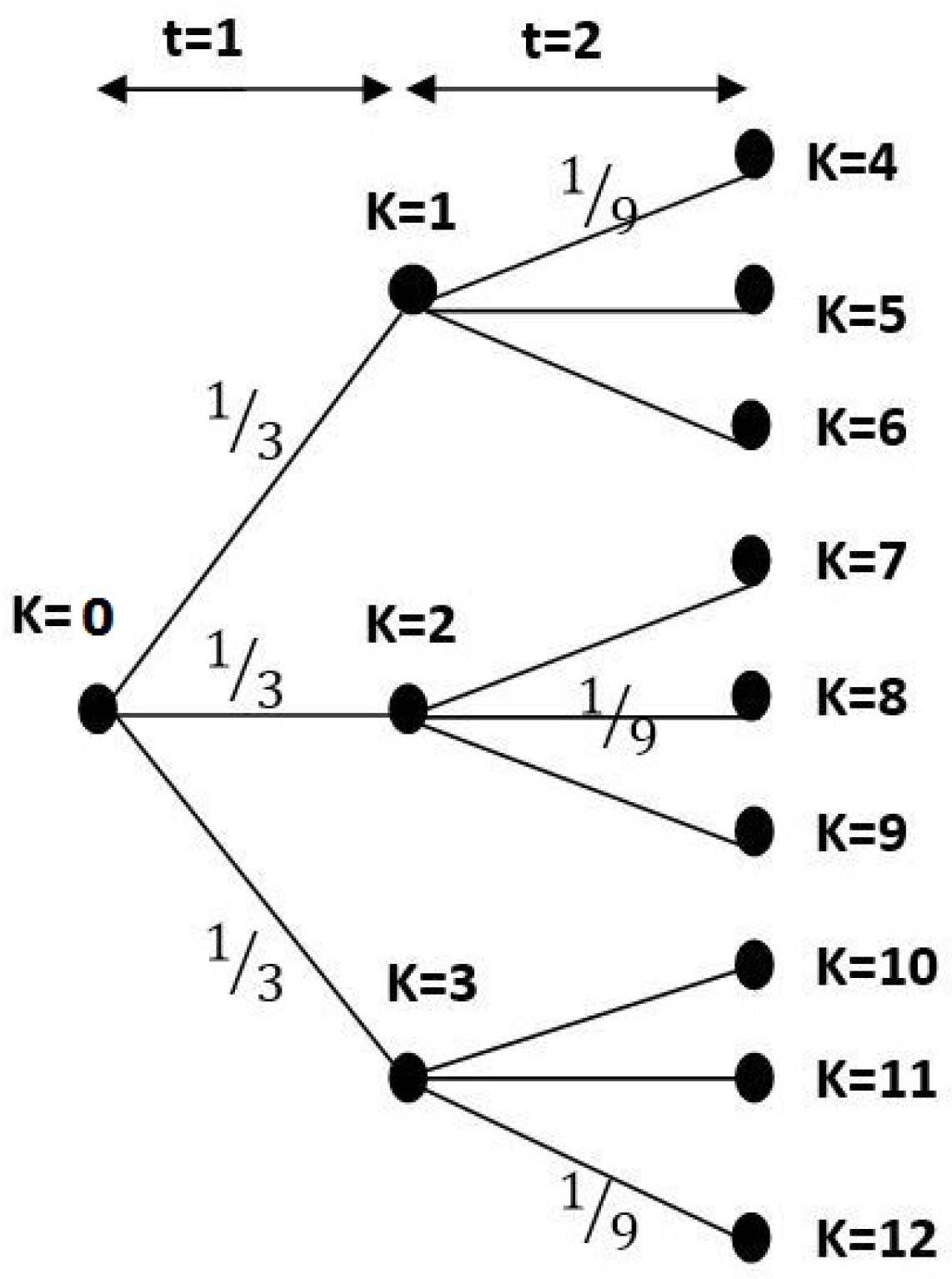
Figure 1. Scenario tree for two-time stages and 3 branches for each node.
Mathematics 11 03883 g001
Figure 2. Solution under the scenario tree with 4 branches per node.
Mathematics 11 03883 g002
Figure 3. Solution under the scenario tree with 31 branches per node.
Mathematics 11 03883 g003
Figure 4. Lifting scheme for 1 breakpoint (left) and 2 breakpoints (right) on a single uncertain parameter ξ q , t .
Mathematics 11 03883 g004
Figure 5. Illustration of the relation between c o n v ( Ξ ) and its convex overestimation Ξ ^ .
Mathematics 11 03883 g005
Figure 6. y 1 ( ξ 1 ) , y 2 ( ξ 1 , ξ 2 ) solution under 2 breakpoints: ( 1 , 2 ) for ξ 1 , and ( 2 , 4 ) for ξ 2 .
Mathematics 11 03883 g006
Figure 7. Partitioning of the two-dimensional uncertainty set (left figure) and scenario tree representation (right figure).
Mathematics 11 03883 g007
Figure 8. Solution from finite adaptability method using two breakpoints for each parameter.
Mathematics 11 03883 g008
Figure 9. Solution from finite adaptability method using 29 breakpoints for each parameter.
Mathematics 11 03883 g009
Figure 10. Comparison of lifting and finite adaptability method using the same fixed breakpoints setting (first configuration).
Mathematics 11 03883 g010
Figure 11. Comparison of lifting and finite adaptability method using the same fixed breakpoints setting (second configuration).
Mathematics 11 03883 g011
Figure 12. Comparison of the solution from the lifting method using fixed breakpoints and optimized breakpoints.
Mathematics 11 03883 g012
Figure 13. Comparison of solutions from finite adaptability method using fixed breakpoints and optimized breakpoints.
Mathematics 11 03883 g013
Table 1. Results of scenario tree method for the illustrating example.
BranchesObjectiveRun TimeBinary Variables
4−1.6250.032 s20
11−1.5620.041 s132
31−1.6050.078 s993
99−1.5940.433 s9900
Table 2. Solution from lifting method with different numbers of fixed breakpoints.
Number of BreakpointsNumber of VariablesObjectiveRun Time
15 Integer, 159 continuous−1.0000.022 s
28 Integer, 199 continuous−1.3330.078 s
929 Integer, 514 continuous−1.3330.094 s
Table 3. Solution statistics for variable breakpoint lifting.
Number of BreakpointsNumber of VariablesObjectiveRun Time
15 integer, 513 continuous−1.3331.075 s
28 integer, 876 continuous−1.3332.375 s
929 integer, 6112 continuous−1.3332 min, 14 s
Table 4. Solution of finite adaptability method.
Number of BreakpointsNumber of VariablesObjectiveRun Time
218 binary, 109 continuous−1.4440.015 s
9200 binary, 1201 continuous−1.5100.016 s
291800 binary, 10,801 continuous−1.5890.078 s
Table 5. Variable breakpoint partitioning applied to the illustrating example.
Number of BreakpointsNumber of VariablesObjectiveRun Time
18 binary, 83 continuous−1.3330.682 s
218 binary, 180 continuous−1.5000.604 s
332 binary, 315 continuous−1.5280.928 s
572 binary, 699 continuous−1.56218 min 54 s
Table 6. Inventory problem parameters.
First Configuration
N c z c y c h q y q z
22347.57.5
Second Configuration
N c z c y c h q y q z
325655
Table 7. Results for the partitioning method, first configuration.
T, BrObjectiveRun TimeOpt. GapConstraintsCont. VarsDiscrete Vars
T = 2, Br = 1118.08.42 s0897120
T = 2, Br = 2100.58.8 s019715140
T = 2, Br = 396.438.64 s034926368
T = 2, Br = 587.768.533 s0785583148
T = 2, Br = 785.308.48 s013971031260
T = 2, Br = 1579.538.69 s0560541031028
T = 5, Br = 1378.178.82 s032442253330
T = 5, Br = 2320.309.52 s024,79717,0232440
T = 5, Br = 3291.7011.65 s0104,80071,69310,250
T = 5, Br = 5272.341 min 22 s0797,828544,33377,770
T = 5, Br = 7243.1025 min 10 s03,365,7522,293,773327,690
T = 10, Br = 1903.1519.22 s0364,561245,78320,500
Note: “T” denotes the number of stages, “Br” denotes the number of breakpoints.
Table 8. Results for the partitioning method, second configuration.
T, BrObjectiveRun TimeOpt. GapConstraintsCont. VarsDiscrete Vars
T = 2, Br = 1124.58.41 s0918130
T = 2, Br = 3108.568.78 s0361297102
T = 2, Br = 5101.378.71 s0815657222
T = 2, Br = 797.078.40 s014531161390
T = 2, Br = 1593.218.49 s0584546171542
T = 5, Br = 1476.758.9 s033422418495
T = 5, Br = 3359.4511.94 s0108,55676,81815,375
T = 5, Br = 5323.291 min 56 s0827,378583,218116,655
T = 5, Br = 7291.7038 min 16 s03,492,1442,457,618491,535
T = 10, Br = 11184.0721.4 s0372,755256,03330,750
Table 9. Results for the lifting method, first configuration.
T, BrObjectiveRun TimeOpt. GapConstraintsCont. VarsDiscrete Vars
T = 2, Br = 1118.00.04 s040527714
T = 2, Br = 2118.00.04 s054536320
T = 2, Br = 3103.00.06 s068544926
T = 2, Br = 599.250.08 s096562138
T = 2, Br = 799.250.27 s0124579350
T = 2, Br = 1594.0917.42 s02365148198
T = 5, Br = 1403.250.11 s02358160350
T = 5, Br = 2399.506.30 s03233213380
T = 5, Br = 3390.1229.53 s041082663110
T = 5, Br = 5378.871 h 57 min058583723170
T = 5, Br = 7371.3710 h6.05%76084783230
T = 5, Br = 15369.0310 h22.98%14,6089023470
T = 10, Br = 11115.2518.83 s010,8935768155
T = 10, Br = 31012.1210 h6.13%16,21310,473370
T = 10, Br = 51004.6210 h12.83%23,21314,693590
T = 10, Br = 71004.6210 h20.23%30,21318,913810
T = 10, Br = 151073.0610 h25.76%58,21335,5571454
T = 20, Br = 13575.010 h1.55%36,42324,813610
T = 20, Br = 33421.2510 h11.4%64,42341,8731670
T = 20, Br = 53441.8710 h19.68%92,42358,8892686
T = 20, Br = 73892.8110 h29.35%120,42375,0692866
T = 20, Br = 154549.9910 h21.66%232,423139,6573454
Table 10. Results for lifting method, second configuration.
T, BrObjectiveRun TimeOpt. GapConstraintsCont. VarsDiscrete Vars
T = 2, Br = 1124.50.11 s056538821
T = 2, Br = 3118.250.11 s095763039
T = 2, Br = 5107.620.23 s0134987257
T = 2, Br = 7107.621.38 s01741111475
T = 2, Br = 15107.6218 min 52 s033092082147
T = 5, Br = 1498.00.13 s03298224875
T = 5, Br = 3461.7526 min 1 s057483738165
T = 5, Br = 5433.010 h2.64%81985228255
T = 5, Br = 7418.6210 h6.28%10,6486718345
T = 5, Br = 15409.8710 h23.56%20,44812,678705
T = 10, Br = 113063.7 s012,8938768225
T = 10, Br = 31202.2510 h5.64%22,69314,698555
T = 10, Br = 51149.1210 h11.95%32,49320,628885
T = 10, Br = 71196.6210 h19.27%42,29326,5581215
T = 10, Br = 151309.1210 h26.77%81,49349,9242181
T = 20, Br = 14456.5210 h3.27%50,98334,798915
T = 20, Br = 34091.2410 h9.5%90,18358,7882505
T = 20, Br = 54006.2510 h19.27%129,38382,7124029
T = 20, Br = 74984.3710 h31.27%168,583105,3824299
T = 20, Br = 156457.1810 h27.51%325,383195,8645181
Table 11. Results for lifting method with breakpoint optimization, first configuration.
T, BrObjectiveRun TimeOpt. GapConstraintsCont. VarsDiscrete Vars
T = 2, Br = 194.075.98 s075663014
T = 2, Br = 294.072 min 40 s01212103220
T = 2, Br = 390.9548 min 48 s01764153026
T = 2, Br = 590.9410 h15.27%3156281438
T = 2, Br = 790.9410 h32.03%4932448250
T = 2, Br = 1594.0210 h48.63%15,87614,99498
T = 5, Br = 1383.375 h19.26%4311356150
T = 5, Br = 2384.5510 h34.93%7056596180
T = 5, Br = 3428.5610 h49.75%10,4019861110
T = 5, Br = 5479.4210 h62.52%18,89116,761170
T = 10, Br = 11089.2310 h30.6%16,71613,766150
T = 10, Br = 21126.1310 h49.30%27,55623,216260
Table 12. Results for partitioning method with breakpoint optimization, first configuration.
T, BrObjectiveRun TimeOpt. GapConstraintsCont. VarsDiscrete Vars
T = 2, Br = 194.071.92 s013711720
T = 2, Br = 286.261 min 47 s029724940
T = 2, Br = 380.0110 h1.28%52143368
T = 2, Br = 578.0610 h2.72%1161957148
T = 2, Br = 779.0310 h34.61%20571689260
T = 2, Br = 15101.6610 h56.63%820166971028
T = 5, Br = 1371.8610 h17.22%38722876330
Disclaimer/Publisher’s Note: The statements, opinions and data contained in all publications are solely those of the individual author(s) and contributor(s) and not of MDPI and/or the editor(s). MDPI and/or the editor(s) disclaim responsibility for any injury to people or property resulting from any ideas, methods, instructions or products referred to in the content.