_Constantinou_Generalis.png)

Improved Power Series Solution of Transversely Loaded Hollow Annular Membranes: Simultaneous Modification of Out-of-Plane Equilibrium Equation and Radial Geometric Equation

Abstract
:1. Introduction
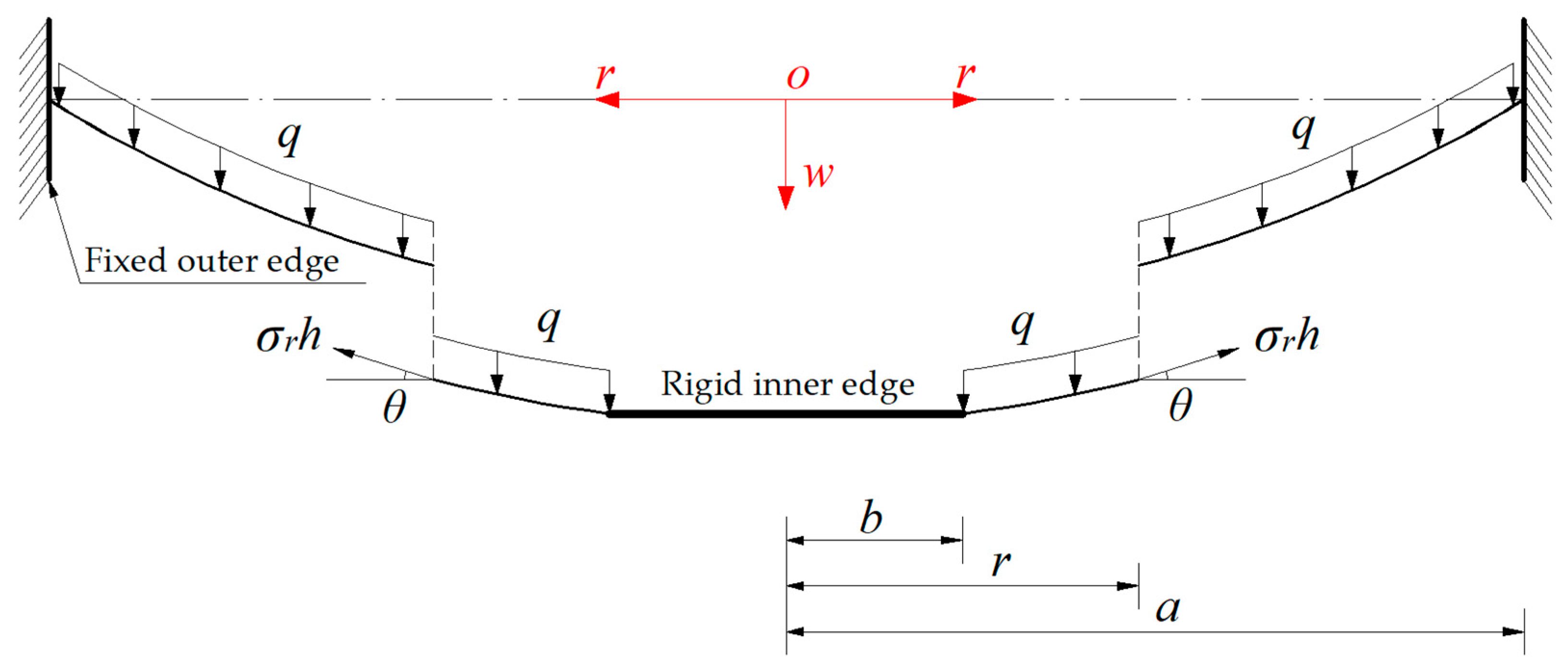
2. Membrane Equation and Solution
3. Results and Discussions
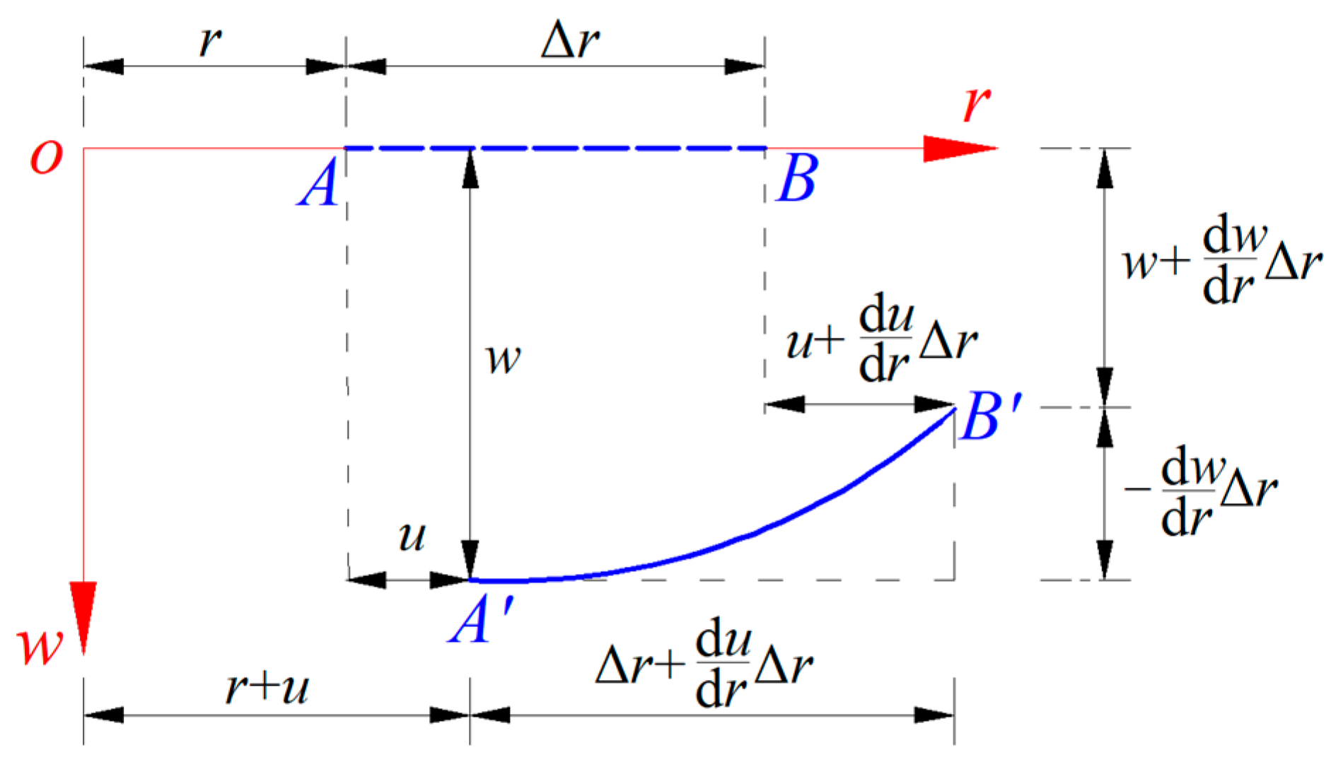
3.1. The Reason Why the Classical Geometric Equations Induce Errors
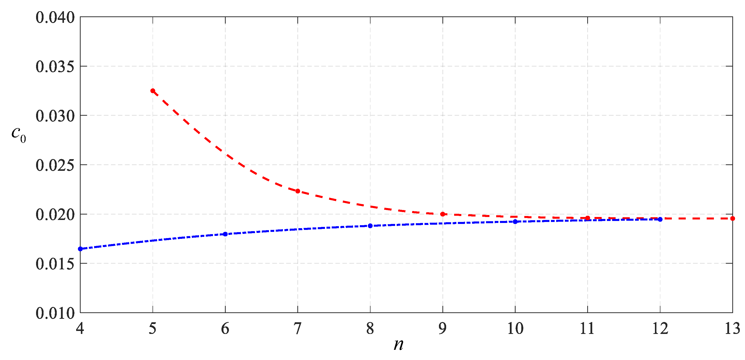
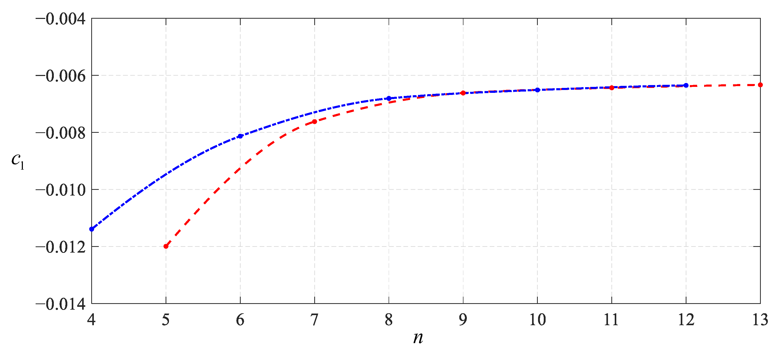
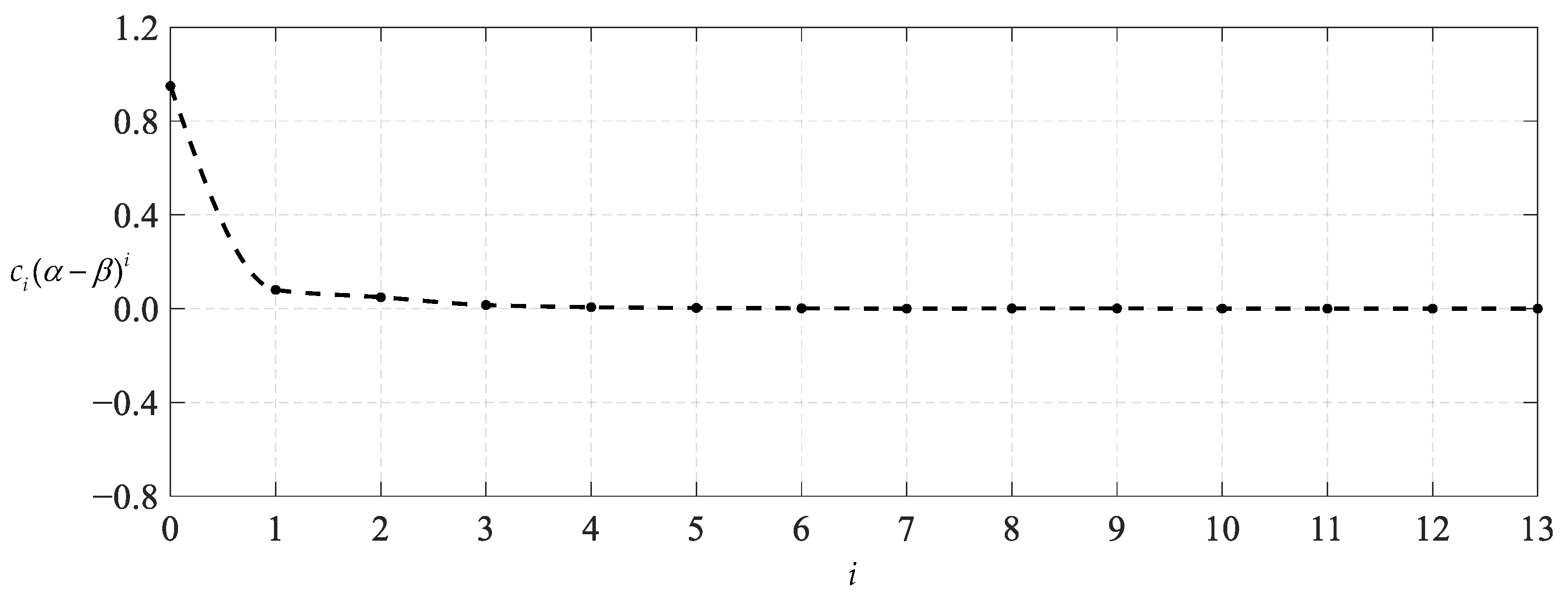
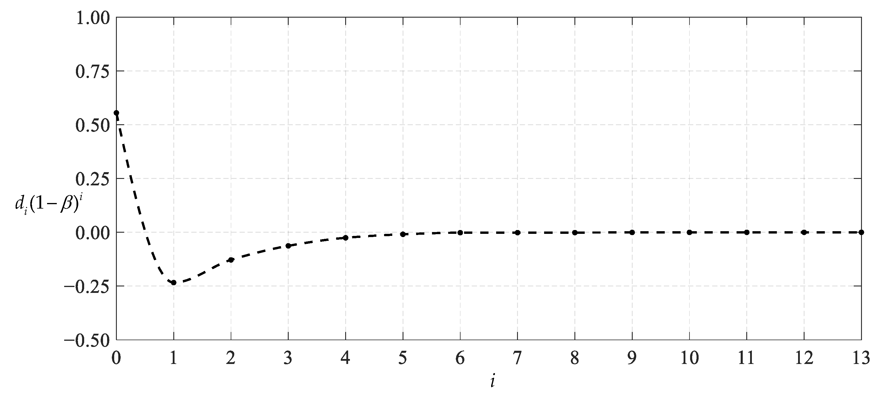
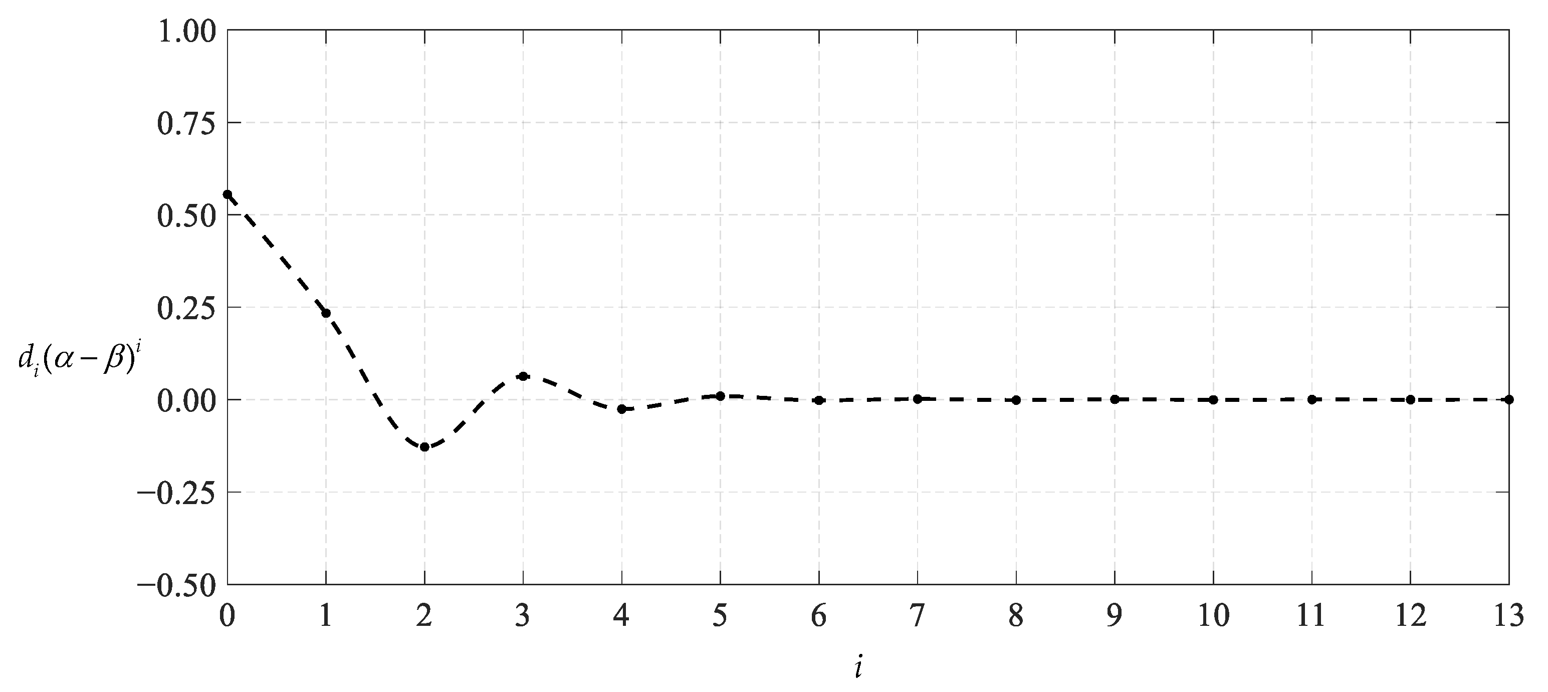
3.2. Convergence Analysis of Power Series Solutions
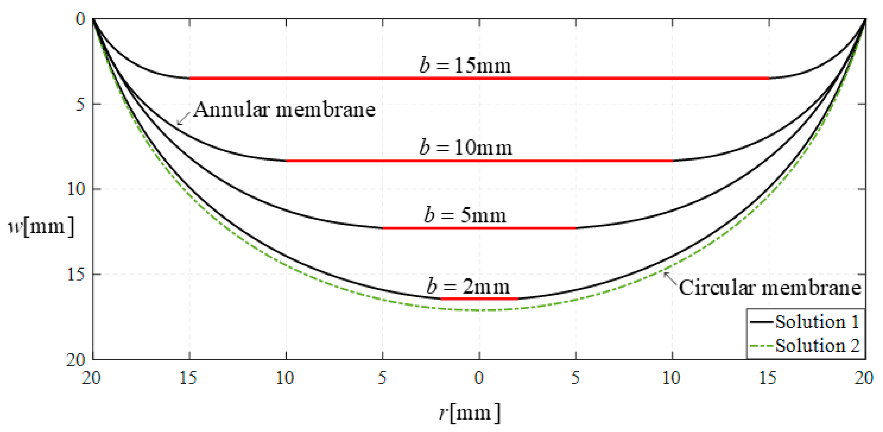
3.3. Asymptotic Behavior from Annular Membrane Solution to Circular Membrane Solution
3.4. Comparison between Hollow Annular Membrane Solutions before and after Improvement
3.5. Difference in Shell Design between Hollow and Solid Annular Membrane Solutions
4. Concluding Remarks
Author Contributions
Funding
Data Availability Statement
Conflicts of Interest
Appendix A
References
- Cao, Z.; Tao, L.; Akinwande, D.; Huang, R.; Liechti, K.M. Mixed-mode traction-separation relations between graphene and copper by blister tests. Int. J. Solids Struct. 2016, 84, 147–159. [Google Scholar] [CrossRef]
- Sun, J.Y.; Qian, S.H.; Li, Y.M.; He, X.T.; Zheng, Z.L. Theoretical study of adhesion energy measurement for film/substrate interface using pressurized blister test: Energy release rate. Measurement 2013, 46, 2278–2287. [Google Scholar] [CrossRef]
- Ma, Y.; Wang, G.R.; Chen, Y.L.; Long, D.; Guan, Y.C.; Liu, L.Q.; Zhang, Z. Extended Hencky solution for the blister test of nanomembrane. Extrem. Mech. Lett. 2018, 22, 69–78. [Google Scholar] [CrossRef]
- Delfani, M.R. Nonlinear elasticity of monolayer hexagonal crystals: Theory and application to circular bulge test. Eur. J. Mech. A Solid. 2018, 68, 117–132. [Google Scholar] [CrossRef]
- Dai, Z.; Lu, N. Poking and bulging of suspended thin sheets: Slippage, instabilities, and metrology. J. Mech. Phys. Solids 2021, 149, 104320. [Google Scholar] [CrossRef]
- Gutscher, G.; Wu, H.C.; Ngaile, G.; Altan, T. Determination of flow stress for sheet metal forming using the viscous pressure bulge (VPB) test. J. Mater. Process Technol. 2004, 146, 1–7. [Google Scholar] [CrossRef]
- Napolitanno, M.J.; Chudnovsky, A.; Moet, A. The constrained blister test for the energy of interfacial adhesion. J. Adhes. Sci. Technol. 1988, 2, 311–323. [Google Scholar] [CrossRef]
- Zhu, T.T.; Müftü, S.; Wan, K.T. One-dimensional constrained blister test to measure thin film adhesion. J. Appl. Mech. T ASME 2018, 85, 054501. [Google Scholar] [CrossRef]
- Pervier, M.L.A.; Hammond, D.W. Measurement of the fracture energy in mode I of atmospheric ice accreted on different materials using a blister test. Eng. Fract. Mech. 2019, 214, 223–232. [Google Scholar] [CrossRef]
- Zhu, T.T.; Li, G.X.; Müftü, S.; Wan, K.T. Revisiting the constrained blister test to measure thin film adhesion. J. Appl. Mech. T ASME 2017, 84, 071005. [Google Scholar] [CrossRef]
- Meng, G.Q.; Ko, W.H. Modeling of circular diaphragm and spreadsheet solution programming for touch mode capacitive sensors. Sens. Actuators A 1999, 75, 45–52. [Google Scholar] [CrossRef]
- Lee, H.Y.; Choi, B. Theoretical and experimental investigation of the trapped air effect on air-sealed capacitive pressure sensor. Sens. Actuators A 2015, 221, 104–114. [Google Scholar] [CrossRef]
- Mishra, R.B.; Khan, S.M.; Shaikh, S.F.; Hussain, A.M.; Hussain, M. Low-cost foil/paper based touch mode pressure sensing element as artificial skin module for prosthetic hand. In Proceedings of the 2020 3rd IEEE International Conference on Soft Robotics (RoboSoft), New Haven, CT, USA, 15 May–15 July 2020; pp. 194–200. [Google Scholar]
- Molla-Alipour, M.; Ganji, B.A. Analytical analysis of mems capacitive pressure sensor with circular diaphragm under dynamic load using differential transformation method (DTM). Acta Mech. Solida Sin. 2015, 28, 400–408. [Google Scholar] [CrossRef]
- Wang, J.; Lou, Y.; Wang, B.; Sun, Q.; Zhou, M.; Li, X. Highly sensitive, breathable, and flexible pressure sensor based on electrospun membrane with assistance of AgNW/TPU as composite dielectric layer. Sensors 2020, 20, 2459. [Google Scholar] [CrossRef] [PubMed]
- Lian, Y.S.; Sun, J.Y.; Zhao, Z.H.; Li, S.Z.; Zheng, Z.L. A refined theory for characterizing adhesion of elastic coatings on rigid substrates based on pressurized blister test methods: Closed-form solution and energy release rate. Polymers 2020, 12, 1788. [Google Scholar] [CrossRef] [PubMed]
- Li, X.; Sun, J.Y.; Shi, B.B.; Zhao, Z.H.; He, X.T. A theoretical study on an elastic polymer thin film-based capacitive wind-pressure sensor. Polymers 2020, 12, 2133. [Google Scholar] [CrossRef] [PubMed]
- Jindal, S.K.; Varma, M.A.; Thukral, D. Comprehensive assessment of MEMS double touch mode capacitive pressure sensor on utilization of SiC film as primary sensing element: Mathematical modelling and numerical simulation. Microelectron. J. 2018, 73, 30–36. [Google Scholar] [CrossRef]
- Shu, J.F.; Yang, R.R.; Chang, Y.Q.; Guo, X.Q.; Yang, X. A flexible metal thin film strain sensor with micro/nano structure for large deformation and high sensitivity strain measurement. J. Alloys Compd. 2021, 879, 160466. [Google Scholar] [CrossRef]
- Zhang, D.Z.; Jiang, C.X.; Tong, J.; Zong, X.Q.; Hu, W. Flexible Strain Sensor Based on Layer-by-Layer Self-Assembled Graphene/Polymer Nanocomposite Membrane and Its Sensing Properties. J. Electron. Mater. 2018, 47, 2263–2270. [Google Scholar] [CrossRef]
- Han, X.D.; Li, G.; Xu, M.H.; Ke, X.; Chen, H.Y.; Feng, Y.J.; Yan, H.P.; Li, D.T. Differential MEMS capacitance diaphragm vacuum gauge with high sensitivity and wide range. Vacuum 2021, 191, 110367. [Google Scholar] [CrossRef]
- Sun, J.-Y.; Zhang, Q.; Wu, J.; Li, X.; He, X.-T. Large Deflection Analysis of Peripherally Fixed Circular Membranes Subjected to Liquid Weight Loading: A Refined Design Theory of Membrane Deflection-Based Rain Gauges. Materials 2021, 14, 5992. [Google Scholar] [CrossRef] [PubMed]
- Moghaddam, B.P.; Tenreiro Machado, J.A. A computational approach for the solution of a class of variable-order fractional integro-differential equations with weakly singular kernels. Fract. Calc. Appl. Anal. 2017, 20, 1023–1042. [Google Scholar] [CrossRef]
- Mokhtary, P.; Moghaddam, B.P.; Lopes, A.M.; Tenreiro Machado, J.A. A computational approach for the non-smooth solution of non-linear weakly singular Volterra integral equation with proportional delay. Numer. Algorithms 2020, 83, 987–1006. [Google Scholar] [CrossRef]
- Hencky, H. On the stress state in circular plates with vanishing bending stiffness. Z. Angew. Math. Phys. 1915, 63, 311–317. [Google Scholar]
- Alekseev, S.A. Elastic circular membranes under the uniformly distributed loads. Eng. Corpus 1953, 14, 196–198. [Google Scholar]
- Chien, W.Z.; Wang, Z.Z.; Xu, Y.G.; Chen, S.L. The symmetrical deformation of circular membrane under the action of uniformly distributed loads in its central portion. Appl. Math. Mech. 1981, 2, 599–612. [Google Scholar]
- Huang, P.F.; Song, Y.P.; Li, Q.; Liu, X.Q.; Feng, Y.Q. A theoretical study of circular orthotropic membrane under concentrated load: The relation of load and deflection. IEEE Access 2020, 8, 126127–126137. [Google Scholar] [CrossRef]
- Zhang, C.H.; Fan, L.J.; Tan, Y.F. Sequential limit analysis for clamped circular membranes involving large deformation subjected to pressure load. Int. J. Mech. Sci. 2019, 155, 440–449. [Google Scholar] [CrossRef]
- Alekseev, S.A. Elastic annular membranes with a stiff centre under the concentrated force. Eng. Corpus 1951, 10, 71–80. [Google Scholar]
- Sun, J.Y.; Zhang, Q.; Li, X.; He, X.T. Axisymmetric large deflection elastic analysis of hollow annular membranes under transverse uniform loading. Symmetry 2021, 13, 1770. [Google Scholar] [CrossRef]
- Zhang, Q.; Li, X.; He, X.-T.; Sun, J.-Y. Revisiting the Boundary Value Problem for Uniformly Transversely Loaded Hollow Annular Membrane Structures: Improvement of the Out-of-Plane Equilibrium Equation. Mathematics 2022, 10, 1305. [Google Scholar] [CrossRef]
- Bellés, P.; Ortega, N.; Rosales, M.; Andrés, O. Shell form-finding: Physical and numerical design tools. Eng. Struct. 2009, 31, 2656–2666. [Google Scholar] [CrossRef]
- Chiang, Y.-C.; Borgart, A. A form-finding method for membrane shells with radial basis functions. Eng. Struct. 2022, 251, 113514. [Google Scholar] [CrossRef]
- Sakai, Y.; Ohsaki, M.; Adriaenssens, S. A 3-dimensional elastic beam model for form-finding of bending-active gridshells. Int. J. Solids Struct. 2020, 193–194, 328–337. [Google Scholar] [CrossRef]
- Isler, H. New Shapes for Shells. Bull. IASS 1960, 8, C-3. [Google Scholar]
- Isler, H. New Shapes for Shells—Twenty years after. Bull. IASS 1979, 20, 9–26. [Google Scholar]
- Isler, H. Generating Shell Shapes by Physical Experiment. Bull. IASS 1993, 34, 53–63. [Google Scholar]
- Lian, Y.S.; Sun, J.-Y.; Zhao, Z.H.; He, X.-T.; Zheng, Z.L. A Revisit of the Boundary Value Problem for Föppl–Hencky Membranes: Improvement of Geometric Equations. Mathematics 2020, 8, 631. [Google Scholar] [CrossRef]
- Malikan, M.; Eremeyev, V.A. On Nonlinear Bending Study of a Piezo-Flexomagnetic Nanobeam Based on an Analytical-Numerical Solution. Nanomaterials 2020, 10, 1762. [Google Scholar] [CrossRef]
- Li, B.; Zhang, Q.; Li, X.; He, X.-T.; Sun, J.-Y. A Refined Closed-Form Solution for the Large Deflections of Alekseev-Type Annular Membranes Subjected to Uniformly Distributed Transverse Loads: Simultaneous Improvement of Out-of-Plane Equilibrium Equation and Geometric Equation. Mathematics 2022, 10, 2121. [Google Scholar] [CrossRef]


| N | c0 | c1 | d0 |
|---|---|---|---|
| 4 | 0.01646666 | −0.01138984 | 0.10267427 |
| 5 | 0.03249455 | −0.01199211 | 0.04604041 |
| 6 | 0.01796667 | −0.00813265 | 0.08935338 |
| 7 | 0.02232676 | −0.00762124 | 0.06828286 |
| 8 | 0.01880637 | −0.00680932 | 0.08100357 |
| 9 | 0.01998771 | −0.00662006 | 0.07647870 |
| 10 | 0.01923017 | −0.00651388 | 0.07894926 |
| 11 | 0.01970104 | −0.00643829 | 0.07802335 |
| 12 | 0.01960104 | −0.00635337 | 0.07870444 |
| 13 | 0.01955117 | −0.00633490 | 0.07853201 |
| N | c0 | c1 | d0 |
|---|---|---|---|
| 4 | 0.79797871 | −0.44917499 | 0.95536325 |
| 5 | 1.12954782 | −0.40144873 | 0.34060805 |
| 6 | 0.88385455 | −0.29134547 | 0.70383470 |
| 7 | 0.98804969 | −0.26562043 | 0.50138603 |
| 8 | 0.92645754 | −0.22996321 | 0.58732742 |
| 9 | 0.95209407 | −0.22476126 | 0.54151308 |
| 10 | 0.94368571 | −0.21505911 | 0.55933494 |
| 11 | 0.95103284 | −0.21448360 | 0.54489530 |
| 12 | 0.94887115 | −0.21384688 | 0.55189530 |
| 13 | 0.94926763 | −0.21357301 | 0.55497352 |
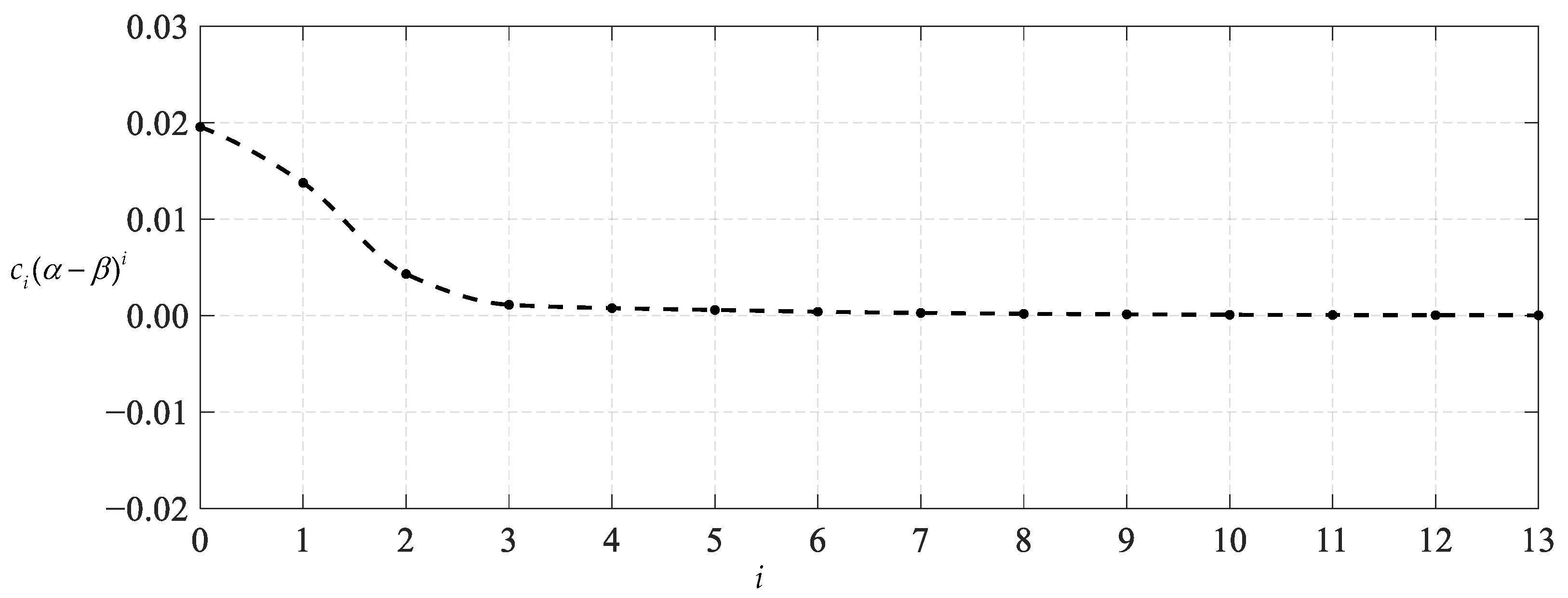
| i | ci(1 − β)i | ci(α − β)i |
|---|---|---|
| 0 | 1.95511735 × 10⁻² | 1.95511735 × 10⁻² |
| 1 | −1.37558825 × 10⁻² | 1.37558825 × 10⁻² |
| 2 | 4.29204384 × 10⁻³ | 4.29204384 × 10⁻³ |
| 3 | −1.11033139 × 10⁻³ | 1.11033138 × 10⁻³ |
| 4 | 7.60061834 × 10⁻⁴ | 7.60061834 × 10⁻⁴ |
| 5 | −5.72876516 × 10⁻⁴ | 5.72876515 × 10⁻⁴ |
| 6 | 3.88148544 × 10⁻⁴ | 3.88148544 × 10⁻⁴ |
| 7 | −2.64333063 × 10⁻⁴ | 2.64333063 × 10⁻⁴ |
| 8 | 1.75184624 × 10⁻⁴ | 1.75184624 × 10⁻⁴ |
| 9 | −1.15724068 × 10⁻⁴ | 1.15724067 × 10⁻⁴ |
| 10 | 7.56547054 × 10⁻⁵ | 7.56547054 × 10⁻⁵ |
| 11 | −4.92739879 × 10⁻⁵ | 4.92739879 × 10⁻⁵ |
| 12 | 3.19117744 × 10⁻⁵ | 3.19117744 × 10⁻⁵ |
| 13 | −2.05943388 × 10⁻⁵ | 2.05943387 × 10⁻⁵ |
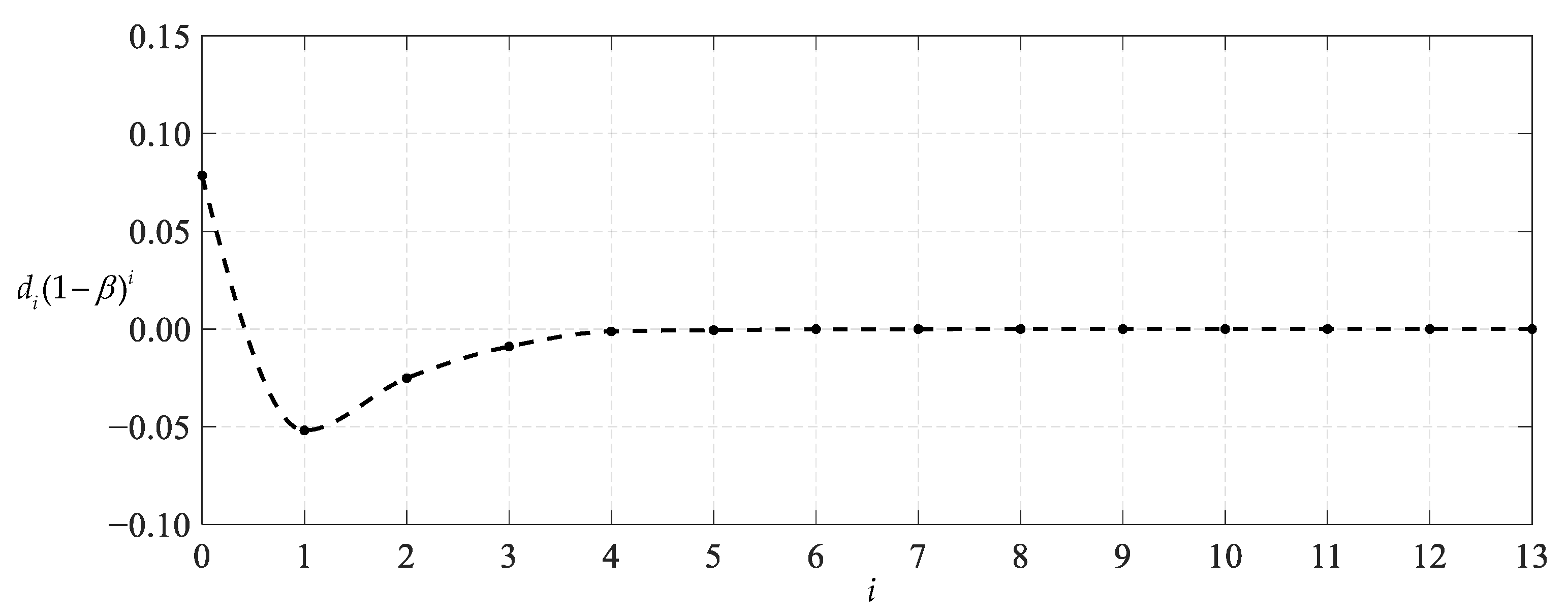
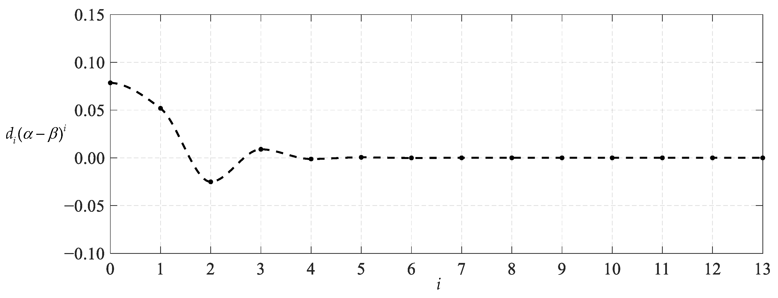
| i | di(1 − β)i | di(α − β)i |
|---|---|---|
| 0 | 7.85320100 × 10⁻² | 7.85320100 × 10⁻² |
| 1 | −5.18652202 × 10⁻² | 5.18652202 × 10⁻² |
| 2 | −2.51092895 × 10⁻² | −2.51092895 × 10⁻² |
| 3 | −8.95332430 × 10⁻³ | 8.95332430 × 10⁻³ |
| 4 | −1.19523279 × 10⁻³ | −1.19523279 × 10⁻³ |
| 5 | −5.55755739 × 10⁻⁴ | 5.55755739 × 10⁻⁴ |
| 6 | −8.24902204 × 10⁻⁵ | −8.24902204 × 10⁻⁵ |
| 7 | −3.32502705 × 10⁻⁵ | 3.32502705 × 10⁻⁵ |
| 8 | −9.76735354 × 10⁻⁶ | −9.76735354 × 10⁻⁶ |
| 9 | −8.57965649 × 10⁻⁶ | 8.57965648 × 10⁻⁶ |
| 10 | −7.80113119 × 10⁻⁶ | −7.80113119 × 10⁻⁶ |
| 11 | −5.55167631 × 10⁻⁶ | 5.55167631 × 10⁻⁶ |
| 12 | −2.77842499 × 10⁻⁶ | −2.77842499 × 10⁻⁶ |
| 13 | −1.58075209 × 10⁻⁶ | 1.580752087 × 10⁻⁶ |
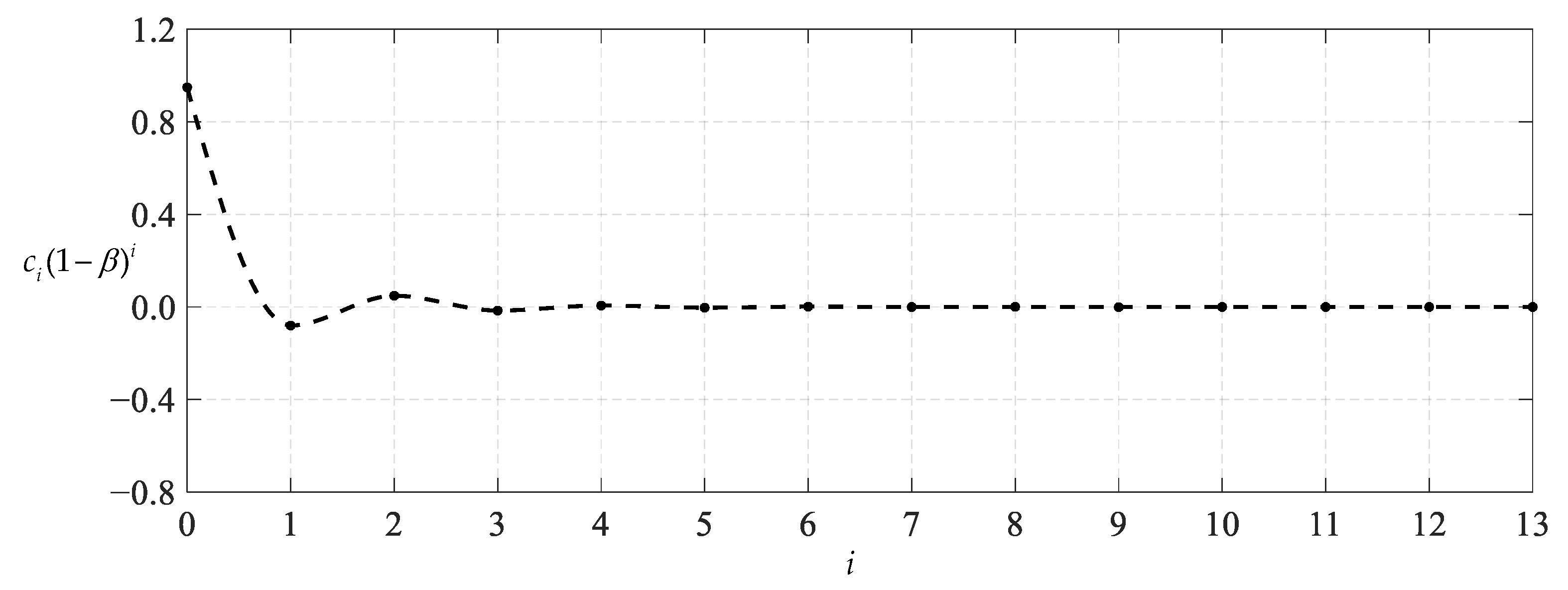
| i | ci(1 − β)i | ci(α − β)i |
|---|---|---|
| 0 | 9.49267634 × 10⁻¹ | 9.49267634 × 10⁻¹ |
| 1 | −8.00898788 × 10⁻² | 8.00898788 × 10⁻² |
| 2 | 4.87742027 × 10⁻² | 4.87742027 × 10⁻² |
| 3 | −1.53845039 × 10⁻² | 1.53845039 × 10⁻² |
| 4 | 6.33479721 × 10⁻³ | 6.33479721 × 10⁻³ |
| 5 | −2.97981462 × 10⁻³ | 2.97981461 × 10⁻³ |
| 6 | 1.61656333 × 10⁻³ | 1.61656332 × 10⁻³ |
| 7 | −1.50452190 × 10⁻⁴ | 1.50452190 × 10⁻⁴ |
| 8 | 7.85985875 × 10⁻⁴ | 7.85985875 × 10⁻⁴ |
| 9 | −6.45125426 × 10⁻⁴ | 6.45125426 × 10⁻⁴ |
| 10 | 1.57480658 × 10⁻⁴ | 1.57480655 × 10⁻⁴ |
| 11 | −9.60276002 × 10⁻⁵ | 9.60276002 × 10⁻⁵ |
| 12 | 4.81002110 × 10⁻⁵ | 4.81002110 × 10⁻⁵ |
| 13 | −3.91803683 × 10⁻⁵ | 3.91803675 × 10⁻⁵ |
| i | di(1 − β)i | di(α − β)i |
|---|---|---|
| 0 | 5.54973520 × 10⁻¹ | 5.54973523 × 10⁻¹ |
| 1 | −2.33806340 × 10⁻¹ | 2.33806340 × 10⁻¹ |
| 2 | −1.28213464 × 10⁻¹ | −1.28213464 × 10⁻¹ |
| 3 | −6.29533088 × 10⁻² | 6.29533087 × 10⁻² |
| 4 | −2.56029287 × 10⁻² | −2.56029287 × 10⁻² |
| 5 | −9.38273495 × 10⁻³ | 9.38273495 × 10⁻³ |
| 6 | −1.91732946 × 10⁻³ | −1.91732946 × 10⁻³ |
| 7 | −1.56968420 × 10⁻³ | 1.56968419 × 10⁻³ |
| 8 | −1.34252446 × 10⁻³ | −1.34252446 × 10⁻³ |
| 9 | −6.19190966 × 10⁻⁴ | 6.19190966 × 10⁻⁴ |
| 10 | −4.07197509 × 10⁻⁴ | −4.07197509 × 10⁻⁴ |
| 11 | −1.92578525 × 10⁻⁴ | 1.92578535 × 10⁻⁴ |
| 12 | −9.27655317 × 10⁻⁵ | −9.27655302 × 10⁻⁵ |
| 13 | −8.84091866 × 10⁻⁵ | 8.84091878 × 10⁻⁵ |
Disclaimer/Publisher’s Note: The statements, opinions and data contained in all publications are solely those of the individual author(s) and contributor(s) and not of MDPI and/or the editor(s). MDPI and/or the editor(s) disclaim responsibility for any injury to people or property resulting from any ideas, methods, instructions or products referred to in the content. |
© 2023 by the authors. Licensee MDPI, Basel, Switzerland. This article is an open access article distributed under the terms and conditions of the Creative Commons Attribution (CC BY) license (https://creativecommons.org/licenses/by/4.0/).
Share and Cite
He, X.-T.; Li, F.-Y.; Sun, J.-Y. Improved Power Series Solution of Transversely Loaded Hollow Annular Membranes: Simultaneous Modification of Out-of-Plane Equilibrium Equation and Radial Geometric Equation. Mathematics 2023, 11, 3836. https://doi.org/10.3390/math11183836
He X-T, Li F-Y, Sun J-Y. Improved Power Series Solution of Transversely Loaded Hollow Annular Membranes: Simultaneous Modification of Out-of-Plane Equilibrium Equation and Radial Geometric Equation. Mathematics. 2023; 11(18):3836. https://doi.org/10.3390/math11183836
Chicago/Turabian StyleHe, Xiao-Ting, Fei-Yan Li, and Jun-Yi Sun. 2023. "Improved Power Series Solution of Transversely Loaded Hollow Annular Membranes: Simultaneous Modification of Out-of-Plane Equilibrium Equation and Radial Geometric Equation" Mathematics 11, no. 18: 3836. https://doi.org/10.3390/math11183836
APA StyleHe, X.-T., Li, F.-Y., & Sun, J.-Y. (2023). Improved Power Series Solution of Transversely Loaded Hollow Annular Membranes: Simultaneous Modification of Out-of-Plane Equilibrium Equation and Radial Geometric Equation. Mathematics, 11(18), 3836. https://doi.org/10.3390/math11183836