
Can a Hand-Held 3D Scanner Capture Temperature-Induced Strain of Mortar Samples? Comparison between Experimental Measurements and Numerical Simulations

 , ,
, ,  , , , , and
Abstract
:1. Introduction
2. Materials and Exposition
3. Methods
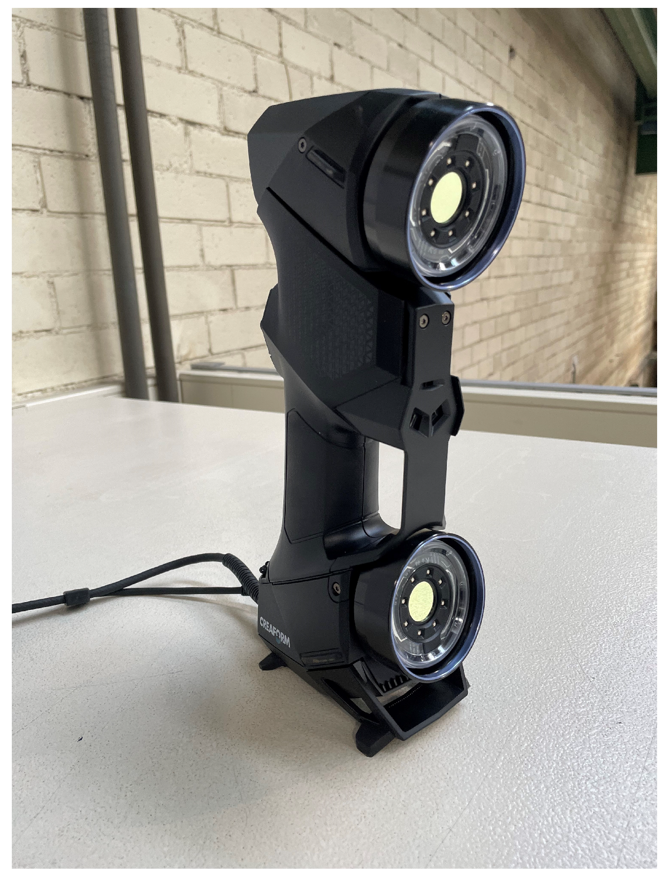
3.1. Three-Dimensional (3D) Scan Data Evaluation
3.2. Numerical Simulation
3.2.1. Mathematical Formulation of the Model
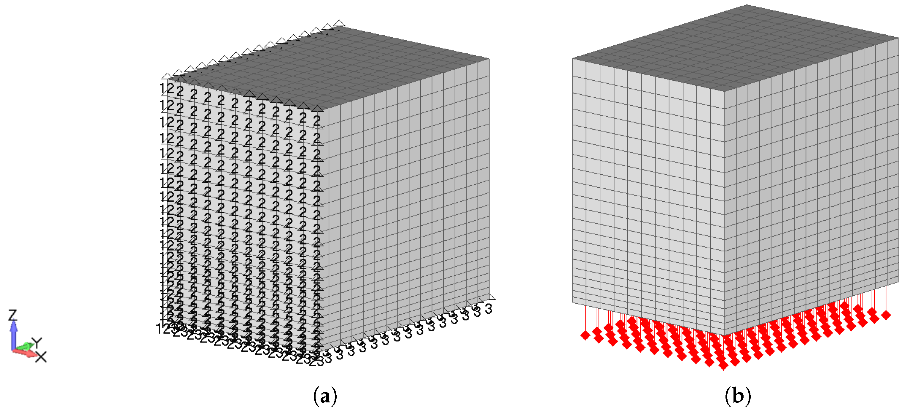
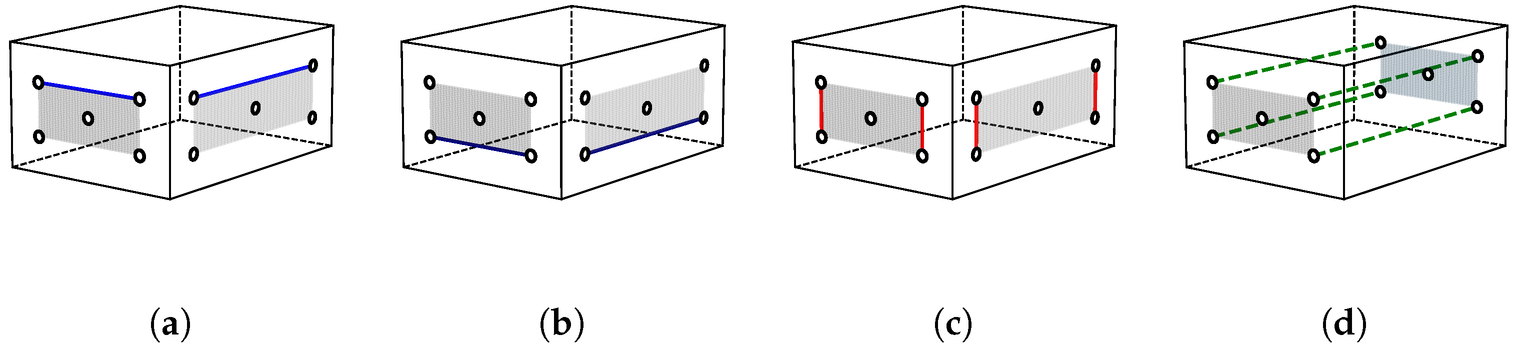
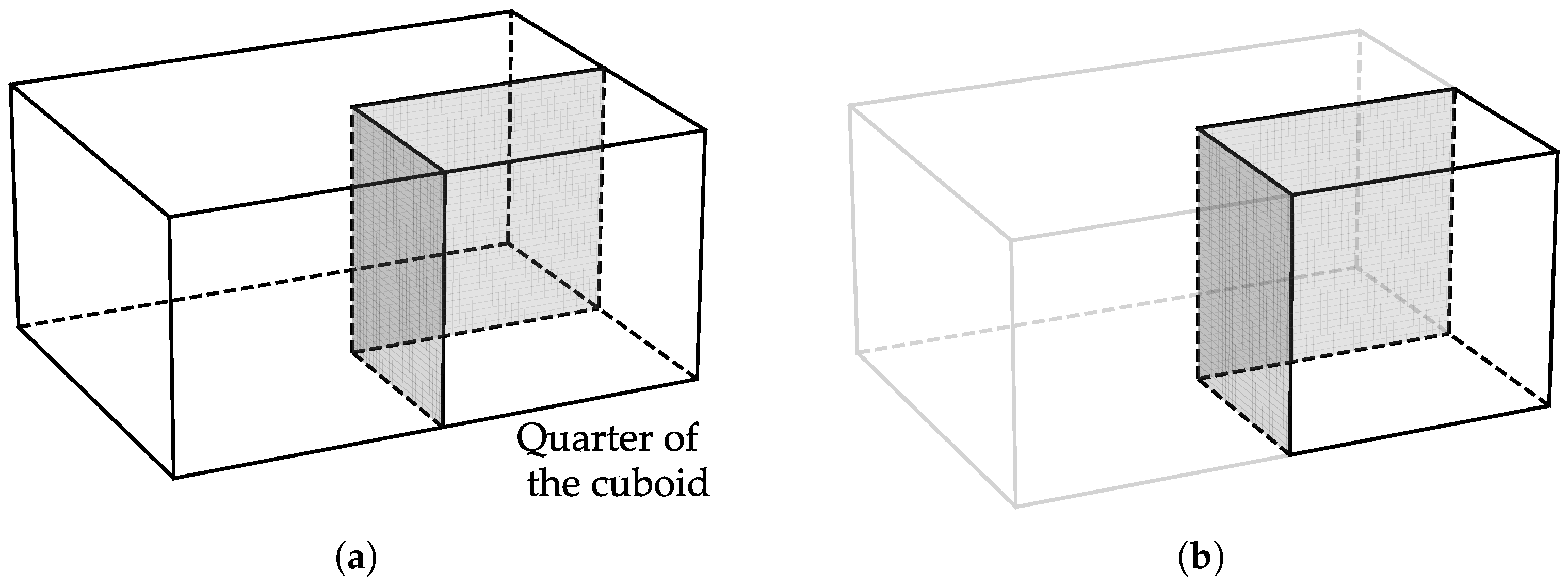
3.2.2. Geometry and FE Discretization
3.2.3. Material Parameters
4. Results and Discussion
4.1. General
4.2. Horizontal Strain
4.3. Vertical Strain
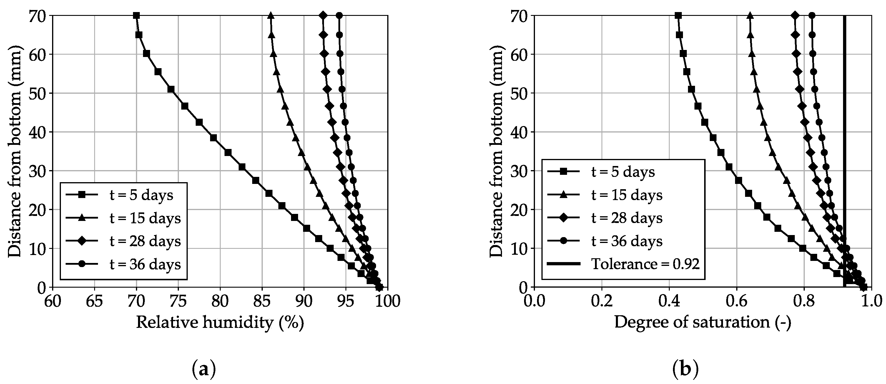
4.4. Strain through the Sample
5. Conclusions
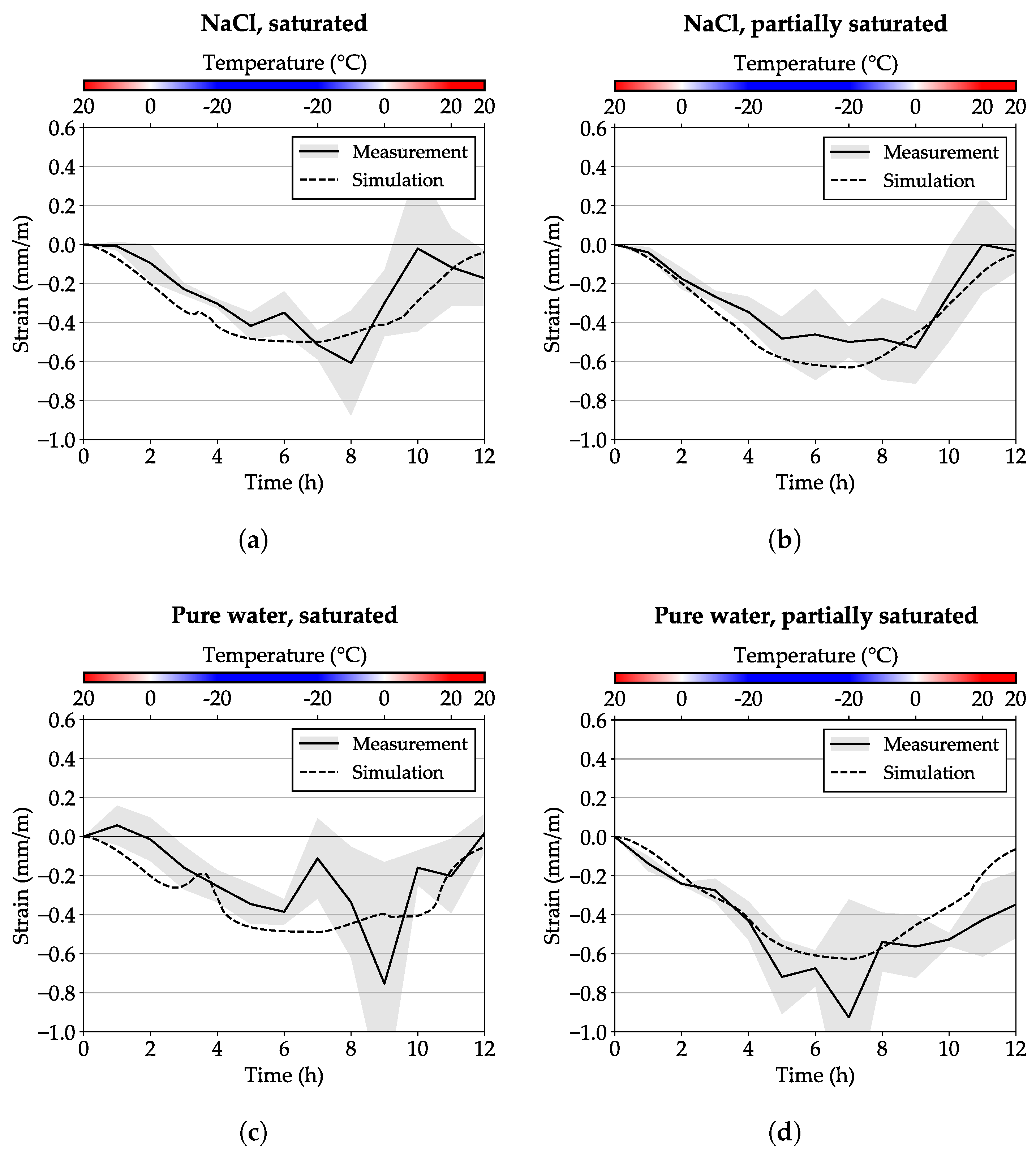
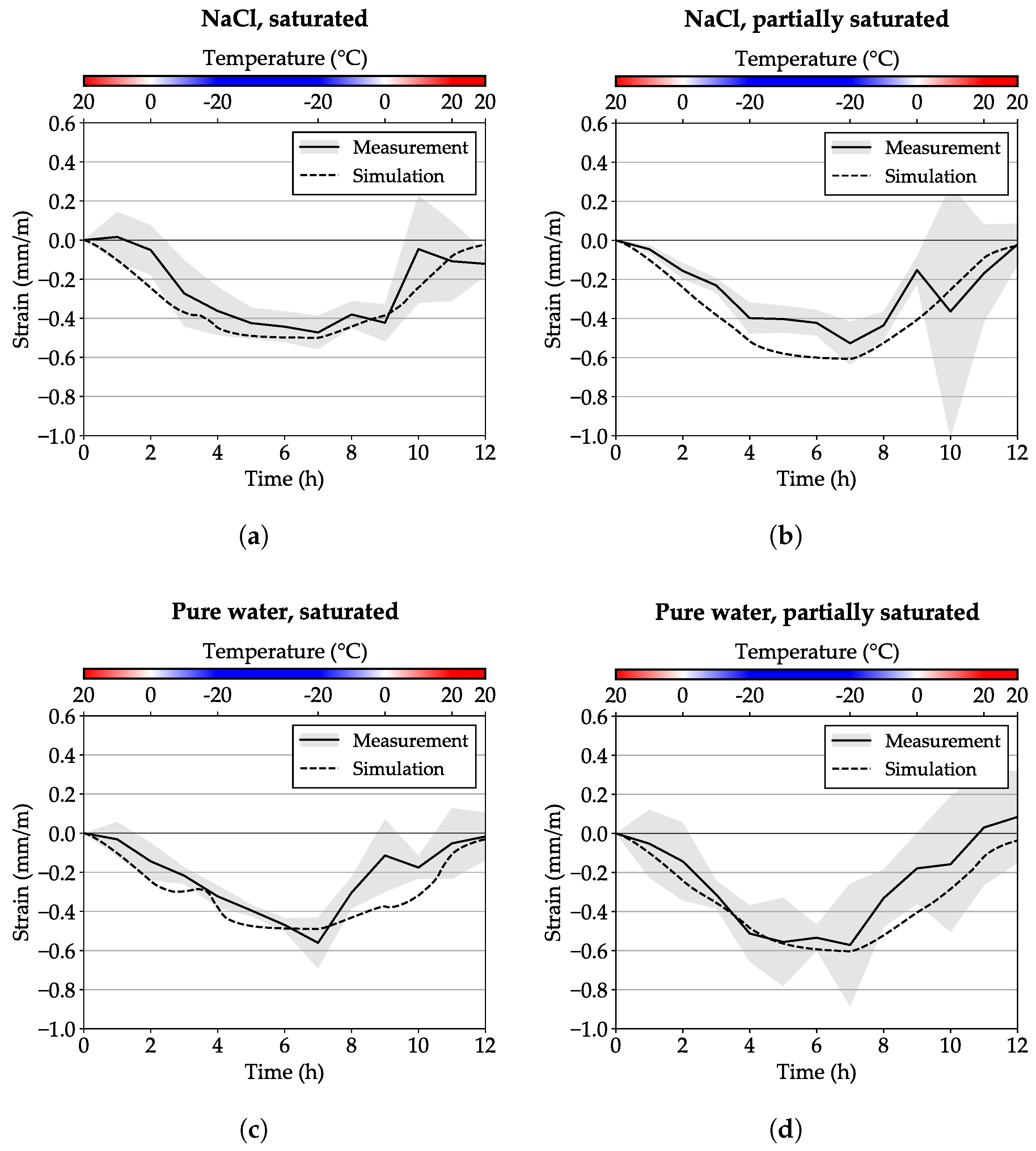
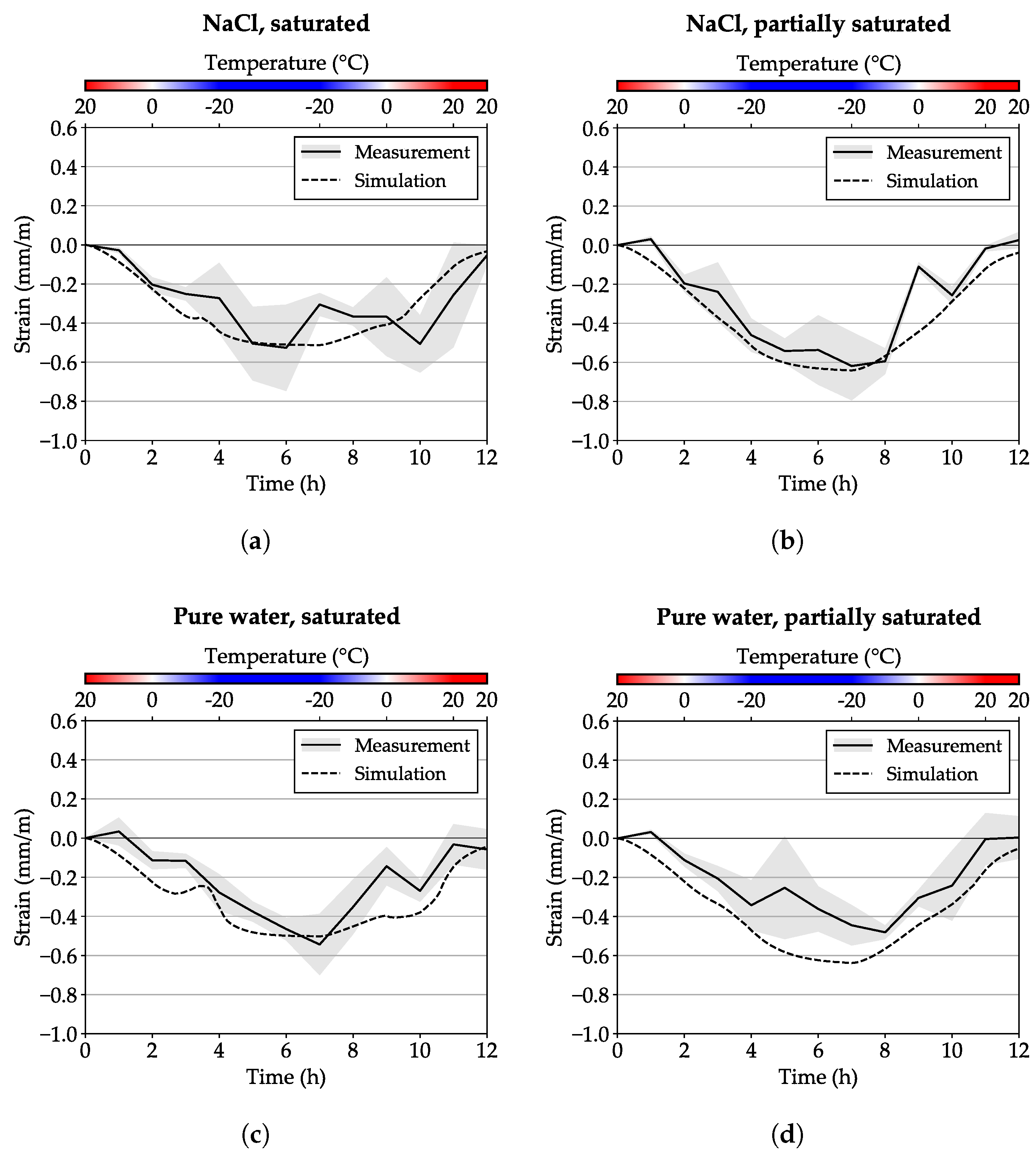
- Saturated samples show a maximum contraction of −0.4 mm/m and partially saturated show a maximum contraction of −0.6 mm/m.
- There are certain limitations of the methodology:
- -
- The methodology is very time consuming due to the fact that the strain measurements are conducted manually.
- -
- Surface effects (freezing of condensated water on the surface) have an influence on the results.
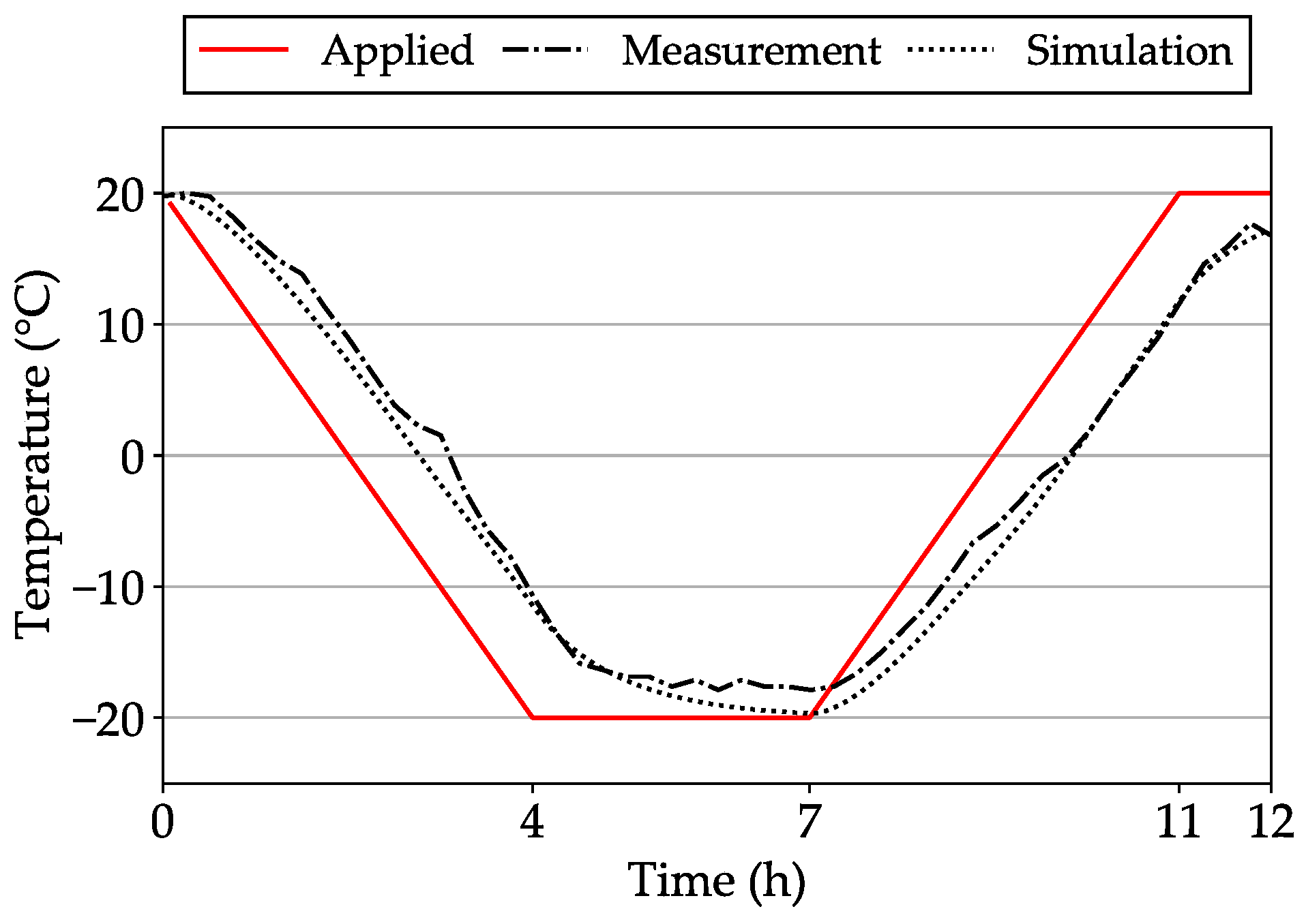
- Comparing the measurement and simulation results, we can generally observe a similar trend of strain behaviour. The results of the thawing phase usually show the most differences. This can be explained by the aforementioned surface effects.
- The 3D-coupled hygro-thermo-mechanical (HTM) model used in this study is capable of reproducing the freezing behaviour of cementitious material in terms of deformation and heat transfer. The model is validated in [23] as well as based on the experimental results presented here. The key calibration parameters are the liquid water permeability, porosity, pore size distribution, and degree of saturation. These parameters play a significant role in the liquid pressure and freezing deformation of the cement paste. Decreasing the liquid water permeability results in higher liquid pressure and consequent deformation.
Author Contributions
Funding
Data Availability Statement
Acknowledgments
Conflicts of Interest
References
- de Brito, J.; Kurda, R. The past and future of sustainable concrete: A critical review and new strategies on cement-based materials. J. Clean. Prod. 2021, 281, 123558. [Google Scholar] [CrossRef]
- Federation internationale du beton. Fib Model Code for Concrete Structures 2010; Wilhelm Ernst & Sohn Verlag fur Architektur und technische Wissenschaften: Berlin, Germany, 2013. [Google Scholar]
- Stark, J.; Wicht, B. Frost- und Frost-Tausalz-Widerstand von Beton. In Dauerhaftigkeit von Beton; Springer: Berlin/Heidelberg, Germany, 2013; pp. 399–471. [Google Scholar] [CrossRef]
- Palecki, S. Hochleistungsbeton unter Frost-Tau-Wechselbelastung:-Schädigung- und Transportmechanismen; Cuvillier Verlag: Göttingen, Germany, 2005. [Google Scholar]
- Powers, T.C.; Copeland, L.E.; Mann, H. Capillary Continuity or Discontinuity in Cement Pastes; Technical Report; Portland Cement Association: Washington, DC, USA, 1959. [Google Scholar]
- German Version CEN/TS 12390-9:2016; Testing Hardened Concrete—Part 9: Freeze–thaw Resistance with De-Icing Salts—Scaling. Beuth Verlag: Berlin, Germany, 2017.
- BAW-Merkblatt Frostprüfung von Beton (MFB); Merkblatt; Bundesanstalt für Wasserbau: Karlsruhe, Germany, 2012.
- Şahin, R.; Taşdemir, M.A.; Gül, R.; Çelik, C. Optimization Study and Damage Evaluation in Concrete Mixtures Exposed to Slow Freeze–Thaw Cycles. J. Mater. Civ. Eng. 2007, 19, 609–615. [Google Scholar] [CrossRef]
- Mao, J.; Ayuta, K. Freeze–thaw resistance of lightweight concrete and aggregate at different freezing rates. J. Mater. Civ. Eng. 2008, 20, 78–84. [Google Scholar] [CrossRef]
- Dombrowski, K.I.; Erfurt, W.; Janssen, D. Identifying D-cracking susceptible aggregates-a comparison of testing procedures. In Proceedings Frost Damage in Concrete; RILEM Publications s.a.r.l.: Cachan, France, 2002; pp. 221–232. [Google Scholar]
- Romero, H.; Enfedaque, A.; Gálvez Ruíz, J.C.; Casati, M. Complementary Testing Techniques Applied to Obtain the Freeze–Thaw Resistance of Concrete; Instituto de Ciencias de la Construcción Eduardo Torroja: Madrid, Spain, 2015. [Google Scholar]
- Haynack, A.; Timothy, J.J.; Kränkel, T.; Gehlen, C. Characterization of cementitious materials exposed to freezing and thawing in combination with de-icing salts using 3D scans. Adv. Eng. Mater. 2023. [Google Scholar] [CrossRef]
- Powers, T.C. A working hypothesis for further studies of frost resistance of concrete. Proc. J. Proc. 1945, 41, 245–272. [Google Scholar]
- Powers, T.C.; Helmuth, R. Theory of volume changes in hardened portland-cement paste during freezing. In Highway Research Board Proceedings, Proceedings of the Thirty-Second Annual Meeting of the Highway Research Board, Washington, DC, USA, 13–16 January, 1953; National Research Council, Highway Research Board: Washington, DC, USA, 1953; Volume 32. [Google Scholar]
- BAŽANT, Z.P.; Chern, J.C.; Rosenberg, A.M.; Gaidis, J.M. Mathematical model for freeze–thaw durability of concrete. J. Am. Ceram. Soc. 1988, 71, 776–783. [Google Scholar] [CrossRef]
- Zuber, B.; Marchand, J. Modeling the deterioration of hydrated cement systems exposed to frost action: Part 1: Description of the mathematical model. Cem. Concr. Res. 2000, 30, 1929–1939. [Google Scholar] [CrossRef]
- Zuber, B.; Marchand, J. Predicting the volume instability of hydrated cement systems upon freezing using poro-mechanics and local phase equilibria. Mater. Struct. 2004, 37, 257–270. [Google Scholar] [CrossRef]
- Yang, R.; Lemarchand, E.; Fen-Chong, T.; Azouni, A. A micromechanics model for partial freezing in porous media. Int. J. Solids Struct. 2015, 75–76, 109–121. [Google Scholar] [CrossRef]
- Timothy, J.J.; Haynack, A.; Kränkel, T.; Gehlen, C. What Is the Internal Pressure That Initiates Damage in Cementitious Materials during Freezing and Thawing? A Micromechanical Analysis. Appl. Mech. 2022, 3, 1288–1298. [Google Scholar] [CrossRef]
- Ožbolt, J. MASA–Macroscopic Space Analysis; Bericht zur Beschreibung des FE-Programmes MASA; Institut für Werkstoffe im Bauwesen, Universität Stuttgart: Stuttgart, Germany, 1998. [Google Scholar]
- Ožbolt, J.; Li, Y.; Kožar, I. Microplane model for concrete with relaxed kinematic constraint. Int. J. Solids Struct. 2001, 38, 2683–2711. [Google Scholar] [CrossRef]
- DIN EN 197-1:2011-11; Cement—Part 1: Composition, Specifications and Conformity Criteria for Common Cements. German Version EN 197-1:2011; Beuth Verlag: Berlin, Germany, 2011.
- Zadran, S.; Ožbolt, J.; Gambarelli, S. Numerical analysis of freezing behaviour of saturated cementitious materials with different amounts of chloride. Materials 2023. [Google Scholar]
- Ožbolt, J.; Oršanić, F.; Balabanić, G. Modeling influence of hysteretic moisture behaviour on distribution of chlorides in concrete. Cem. Concr. Compos. 2016, 67, 73–84. [Google Scholar] [CrossRef]
- Fagerlund, G. Critical Degrees of Saturation at Freezing of Porous and Brittle Materials. Ph.D. Thesis, Division of Building Materials, 1973. [Google Scholar]
- Zeng, Q.; Li, K.; Fen-Chong, T.; Dangla, P. Effect of porosity on thermal expansion coefficient of cement pastes and mortars. Constr. Build. Mater. 2012, 28, 468–475. [Google Scholar] [CrossRef]
- Li, K.; Xu, L.; Stroeven, P.; Shi, C. Water permeability of unsaturated cementitious materials: A review. Constr. Build. Mater. 2021, 302, 124168. [Google Scholar] [CrossRef]
- Li, K.; Stroeven, P.; Stroeven, M.; Sluys, L. Liquid water permeability of partially saturated cement paste assessed by dem-based methodology. In Proceedings of the 11th International Symposium on Brittle Matrix Composites, BMC-11, Warsaw, Poland, 28–30 September 2015; Institute of Fundamental Technological Research PAS: Warsaw, Poland, 2015. [Google Scholar]
- Washburn, E.W. The Dynamics of Capillary Flow. Phys. Rev. 1921, 17, 273–283. [Google Scholar] [CrossRef]
- Canut, M. Pore Structure in Blended Cement Pastes. Ph.D. Thesis, Technical University of Denmark, Lyngby, Denmark, 2011. [Google Scholar]


| Mesh Size (mm) | 0.063 | 0.125 | 0.25 | 0.5 | 1 | 2 |
|---|---|---|---|---|---|---|
| Passing rate (wt.-%) | 0.06 | 0.49 | 19.16 | 48.40 | 75.47 | 100 |
| w/c (-) | Cement (kg/m³) | Water (kg/m³) | Aggregates (kg/m³) |
|---|---|---|---|
| 0.55 | 560 | 308 | 1312 |
| Label | Hardening (d) | Curing (d) | Drying (d) | Capillary Saturation (d) | Water Storage (d) | Total Age (d) |
|---|---|---|---|---|---|---|
| Saturated | 1 | 6 | 21 | - | 140 | 168 |
| Partially saturated | 1 | 6 | 21 | 7 | - | 35 |
| Parameters | w/c = 0.55 |
|---|---|
| Water vapour permeability, (s) | 1.0 × 10 |
| Surface humidity transf. coeff., (m/s) | 2.0 × 10 |
| Property | Symbol | Unit | Value | Reference Source |
|---|---|---|---|---|
| Apparent density | (g/cm³) | 2.5 | Experiment | |
| Poisson’s ratio | - | 0.18 | Literature [23] | |
| w/c | - | - | 0.55 | Experiment |
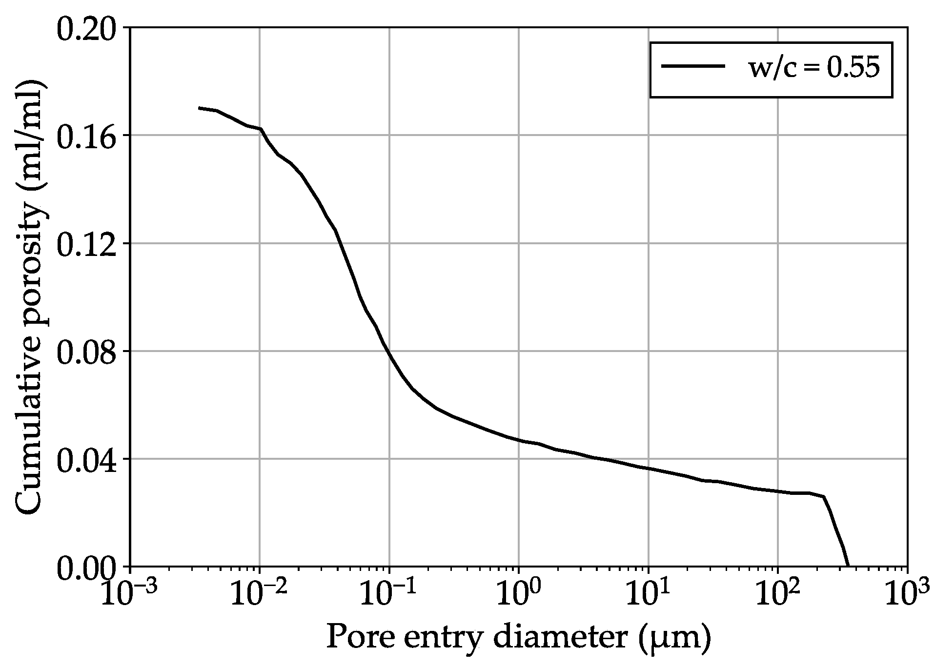
| Total porosity | n | (m³/m³) | 0.17 Figure 10 | Experiment |
| Elastic modulus | E | (GPa) | 30 | Experiment |
| Compressibility modulus of the porous skeleton | (GPa) | Literature [23] | ||
| Compressibility modulus of the solid matrix | (GPa) | Literature [23] | ||
| Biot’s coefficient | b | - | Literature [23] | |
| Pore size distribution | - | (-) | Figure 10 | Experiment |
| Thermal conductivity | (W/m*K) | 2.5 | Experiment | |
| Heat capacity | (J/kg*K) | 937.0 | Experiment | |
| Thermal expansion coefficient | (°C) | 1.64 × 10 | Literature [26] | |
| Liquid water permeability | D | (m²) | Saturated: 6.0 × 10 | Literature [27] |
| Partially Saturated: | ||||
| WSD ≥ 0.92: 3.17 × 10 | ||||
| 0.92 > WSD > 0.80: 1.58 × 10 | ||||
| WSD ≤ 0.80: 1.26 × 10 |
| Variation | Test Solution | Preconditioning |
|---|---|---|
| V1 | NaCl | Saturated |
| V2 | NaCl | Partially saturated |
| V3 | Pure water | Saturated |
| V4 | Pure water | Partially saturated |
Disclaimer/Publisher’s Note: The statements, opinions and data contained in all publications are solely those of the individual author(s) and contributor(s) and not of MDPI and/or the editor(s). MDPI and/or the editor(s) disclaim responsibility for any injury to people or property resulting from any ideas, methods, instructions or products referred to in the content. |
© 2023 by the authors. Licensee MDPI, Basel, Switzerland. This article is an open access article distributed under the terms and conditions of the Creative Commons Attribution (CC BY) license (https://creativecommons.org/licenses/by/4.0/).
Share and Cite
Haynack, A.; Zadran, S.; Timothy, J.J.; Gambarelli, S.; Kränkel, T.; Thiel, C.; Ožbolt, J.; Gehlen, C. Can a Hand-Held 3D Scanner Capture Temperature-Induced Strain of Mortar Samples? Comparison between Experimental Measurements and Numerical Simulations. Mathematics 2023, 11, 3672. https://doi.org/10.3390/math11173672
Haynack A, Zadran S, Timothy JJ, Gambarelli S, Kränkel T, Thiel C, Ožbolt J, Gehlen C. Can a Hand-Held 3D Scanner Capture Temperature-Induced Strain of Mortar Samples? Comparison between Experimental Measurements and Numerical Simulations. Mathematics. 2023; 11(17):3672. https://doi.org/10.3390/math11173672
Chicago/Turabian StyleHaynack, Alexander, Sekandar Zadran, Jithender J. Timothy, Serena Gambarelli, Thomas Kränkel, Charlotte Thiel, Joško Ožbolt, and Christoph Gehlen. 2023. "Can a Hand-Held 3D Scanner Capture Temperature-Induced Strain of Mortar Samples? Comparison between Experimental Measurements and Numerical Simulations" Mathematics 11, no. 17: 3672. https://doi.org/10.3390/math11173672
APA StyleHaynack, A., Zadran, S., Timothy, J. J., Gambarelli, S., Kränkel, T., Thiel, C., Ožbolt, J., & Gehlen, C. (2023). Can a Hand-Held 3D Scanner Capture Temperature-Induced Strain of Mortar Samples? Comparison between Experimental Measurements and Numerical Simulations. Mathematics, 11(17), 3672. https://doi.org/10.3390/math11173672