GRA-Based Dynamic Hybrid Multi-Attribute Three-Way Decision-Making for the Performance Evaluation of Elderly-Care Services

Abstract

As an important branch of modern decision-making theory, multi-attribute decision-making (MADM) plays an important role in various fields. Classic MADM methods can provide a ranking of alternatives, and decision-makers need to evaluate the level subjectively based on the ranking results. Because of the limitation of knowledge, this is likely to lead to potential individual losses. Three-way decision (3WD) theory has good classification ability. Therefore, this paper proposes a dynamic hybrid multi-attribute 3WD (MA3WD) model. First, a new scheme for constructing loss functions is proposed from the perspective of gray relational analysis (GRA), which is an accurate and objective way to describe the relationship between loss functions and attribute values. Then, conditional probabilities are determined by employing the gray relational analysis technique for order preference by similarity to the ideal solution (GRA-TOPSIS). With these discussions, a GRA-based hybrid MA3WD model for a single period is proposed by considering multi-source information. Furthermore, by extending the single-period scenario to a multi-period one, we construct a dynamic hybrid MA3WD model, which can obtain the final three-way decision rules as well as the results of each period and each attribute. Finally, the proposed method is applied to the case of performance evaluation of elderly-care services to demonstrate the effectiveness of the method, and comparative analyses are given to verify the superiority of the proposed method.

1. Introduction

Decision-making is pervasive in our daily life, and multi-attribute decision-making (MADM) is an important part of it. Multi-attribute decision-making has been applied to various fields, including performance evaluation [1,2], risk assessment [3,4], and medical diagnosis [5,6]. With the continuous development of decision theory, classic MADM methods have been progressively proposed, such as TOPSIS [7,8], TODIM [9,10], VIKOR [11,12], etc. However, traditional MADM methods used in most studies are essentially a two-way decision-making procedure [13,14], which only considers two options, namely acceptance and rejection. For instance, when the government makes decisions on the access and exit mechanism of third-party social organizations, the result obtained by MADM methods is to renew a contract or terminate the contract according to the alternative rankings. However, there may be a contradiction where two social organizations with slight differences in evaluation receive opposite decision results, i.e., one is accepted to sign a new contract, while another one is obliged to terminate the contract. To conquer the limitation of traditional MADM methods, this paper introduces three-way decision theory under a multi-attribute decision-making environment. Three-way decision-making, derived from decision-theoretic rough sets (DTRSs), encompasses the ability to objectively classify all alternatives into three regions, i.e., a positive region, a negative region, and a boundary region. Yao provided a reasonable semantic interpretation of these three pairwise disjoint regions from the perspective of cognitive science, corresponding to acceptance, rejection, and non-commitment in the actual decision-making process, respectively [15,16]. Compared with two-way MADM methods, three-way decision-making adds a deferment strategy, which reduces the risk of decision-making. For instance, the two social organizations in the aforementioned example can be classified into a deferment region for further investigation to reduce the loss of misclassification.

In recent years, 3WD has made remarkable achievements in theoretical models and application studies. For theoretical models, many researchers have extended the traditional 3WD model to dynamic environments and proposed improved models, such as sequential three-way decision [17], multi-granulation three-way decision [18], multi-class three-way decision [19], multi-attribute three-way decision [20,21], etc. To solve MADM problems, Jia and Liu [20] proposed a multi-attribute three-way decision model, transforming attribute evaluation values to loss functions in a multi-attribute environment. Zhan et al. [22] introduced the concept of relative utility function, utilized similarity relation to determine conditional probabilities, and proposed a 3WD model in an incomplete fuzzy decision environment. Zhan et al. [23] proposed a MA3WD method based on outranking relations. Huang et al. [24] designed a pair of pre-order relations and further proposed a new method for calculating conditional probabilities. Gao et al. [13] proposed a three-way decision-based target–threat assessment method based on a comprehensive evaluation matrix integrating multi-period information. Subsequently, some researchers incorporated psychological behaviors into the construction of 3WD models. He et al. [25] proposed a behavioral MA3WD model considering the regret-aversion behavior and risk-aversion behavior of human beings. In application studies, 3WD has been widely applied in various practical issues, such as conflict analysis [26,27], medical diagnosis [28,29], investment decisions [30,31], concept analysis [32,33], etc. However, based on the above brief review of 3WD, the existing 3WD methods still have some deficiencies. First, the loss functions and conditional probabilities of 3WD are difficult to determine objectively and scientifically, and lack interpretability; Second, the study of 3WD in a time-dynamic environment is relatively limited, while the time-dynamic environment is the most common type of dynamic decision-making environment in real life.

Due to the complexity of the decision-making environment and the diversity of attributes, exact numbers often struggle to accurately express the fuzzy cognition of decision-makers. Therefore, to describe uncertain information more accurately and reasonably, various fuzzy numbers have been proposed and widely studied, such as interval numbers [34], triangular fuzzy numbers [35], and intuitionistic fuzzy numbers [36]. Moreover, due to the unquantifiable nature of certain attributes, linguistic variables become a powerful tool for describing such information [37]. However, in many practical decision-making problems, it is necessary to use a combination of quantitative and qualitative attribute types. For instance, in the performance evaluation of elderly-care services, attributes such as the number of service programs, professional level, and communication ability are often considered [38,39]. Among them, the number of service programs is a quantitative attribute, which is often expressed by exact numbers; communication ability is a qualitative attribute, often expressed by language variables. Hence, in the decision-making problem with diversity attributes, a single form of information cannot accurately describe all attributes, and it is effective and reliable to adopt a mixed approach using multiple forms of information according to practical needs.

Based on the above analysis of the research subjects, we summarize the motivations and innovations of this paper as follows:

Motivations:

• In the process of constructing the loss function, many existing methods are unreasonable. For instance, in the classical three-way decision theory [15], the loss function is artificially set by the decision-maker, which is not scientific. In addition, Jia and Liu [20] converted the attribute value into a relative loss function in a multi-attribute decision-making environment. This method is also not rational because it uses 1 and 0 as the maximum and minimum of the attribute values in the construction of the relative loss function.
• In the existing studies on MA3WD methods, there is limited consideration of the time-dynamic environment. Most methods are based on decision information from a single period [14,21], which leads to an incomplete evaluation of the objects. Gao et al. [13] proposed a 3WD method based on multi-period evaluation information to address the issue of time dynamics, which is an improvement. However, the model constructed by Gao et al. fails to provide continuous evaluations for objects across different periods.
• Traditional MADM methods have limitations in solving practical problems such as the performance evaluation of elderly-care services. These methods’ essence lies in two-way decision-making, where the outcomes often overlook the necessity of further investigation, leading to potential individual losses.

Innovations:

• A new scheme for constructing loss functions is proposed from the perspective of GRA, which is an accurate and objective way to describe the relationship between loss functions and attribute values.
• Conditional probabilities are estimated based on GRA-TOPSIS, which provides comprehensive and objective results for three-way decisions.
• A GRA-based hybrid MA3WD model considering mixed forms of information is proposed for evaluating objects at a specific period. The model can point out the specific attributes and periods of poor performance of the object so that it accurately improves its shortcomings.
• By extending the single-period scenario to a multi-period one, we construct a GRA-based dynamic hybrid MA3WD model, extending the study of 3WD in a time-dynamic environment.
• This paper introduces the 3WD theory into the performance evaluation of elderly-care services, which provides a scientific and reasonable way to solve this issue.

The remainder of this paper is organized as follows. Section 2 lists the basic concepts of multi-attribute three-way decision-making, the definition of a dynamic hybrid multi-attribute information system, and the basic knowledge of gray relational analysis. Section 3 introduces the concept of gray relational analysis into the construction of loss function, proposes a method to determine conditional probability using GRA-TOPSIS, and further proposes a GRA-based hybrid MA3WD model for a single period. In Section 4, a single-period scenario is extended to a multi-period one, and a dynamic hybrid MA3WD model is proposed using information from the multi-period. In Section 5, the proposed model is applied to the performance evaluation of government purchases of elderly-care services, and its effectiveness is verified through comparative analysis. Section 6 summarizes the final concluding remarks in this paper.

2. Preliminaries

2.1. Multi-Attribute Three-Way Decision (MA3WD)

The three-way decision derived from the DTRSs uses a two-state set and a three-action set to describe the decision process [15]. The set of states $\mathsf{\Omega }=\left\{C,\neg C\right\}$ indicates that an object is in $C$ or not in $C$; the set of actions $A=\left\{a_P,a_B,a_N\right\}$ corresponds to three actions $x\in POS\left(C\right)$, $x\in BND\left(C\right)$, $x\in NEG\left(C\right)$ that are taken when classifying the object $x$, i.e., acceptance, non-commitment, and rejection. When the object $x$ is in different states, the three actions taken produce corresponding losses or risks, which can be represented by the 3 × 2 loss function matrix [15] in

Table 1. The loss functions of a three-way decision.

	$\mathit{C}$	$\neg \mathit{C}$
$a_P$	${\lambda }_{PP}$	${\lambda }_{PN}$
$a_B$	${\lambda }_{BP}$	${\lambda }_{BP}$
$a_N$	${\lambda }_{NP}$	${\lambda }_{NN}$

.

Assume that $\mathrm{Pr}\left(C|\left[x\right]\right)$ represents the conditional probability that an object $x$ belongs to a state $C$, then for any object $x$, the expected loss after taking all actions can be expressed as:

$$R\left(a_P|\left[x\right]\right)={\lambda }_{PP}\mathrm{Pr}\left(C|\left[x\right]\right)+{\lambda }_{PN}\mathrm{Pr}\left(\neg C|\left[x\right]\right)$$

(1)

$$R\left(a_B|\left[x\right]\right)={\lambda }_{BP}\mathrm{Pr}\left(C|\left[x\right]\right)+{\lambda }_{BN}\mathrm{Pr}\left(\neg C|\left[x\right]\right)$$

(2)

$$R\left(a_N\left[x\right]\right)={\lambda }_{NP}\mathrm{Pr}\left(C|\left[x\right]\right)+{\lambda }_{NN}\mathrm{Pr}\left(\neg C|\left[x\right]\right)$$

(3)

Based on the Bayesian theory that the optimal decision is the one with the least cost, the decision rules are deduced as follows:

$$(\mathrm{P}-1) \mathrm{If} R\left(a_P|\left[x\right]\right)\le R\left(a_B|\left[x\right]\right) \mathrm{and} R\left(a_P|\left[x\right]\right)\le R\left(a_N|\left[x\right]\right), \mathrm{decide} x\in POS(C);$$

$$(\mathrm{B}-1) \mathrm{If} R\left(a_B|\left[x\right]\right)\le R\left(a_P|\left[x\right]\right) \mathrm{and} R\left(a_B|\left[x\right]\right)\le R\left(a_N|\left[x\right]\right), \mathrm{decide} x\in BND(C);$$

$$(\mathrm{N}-1) \mathrm{If} R\left(a_N|\left[x\right]\right)\le R\left(a_P|\left[x\right]\right) \mathrm{and} R\left(a_N|\left[x\right]\right)\le R\left(a_B|\left[x\right]\right), \mathrm{decide}x\in NEG(C).$$

Based on the decision rough sets, the decision rules (P-1)~(N-1) are three-way decisions.

Consider the following relationship between the loss functions:

$${\lambda }_{PP}\le {\lambda }_{BP}<{\lambda }_{NP},{\lambda }_{NN}\le {\lambda }_{BN}<{\lambda }_{PN}$$

(4)

Based on the above relationship and $\mathrm{Pr}(C|\left[x\right])+\mathrm{Pr}(\neg C|\left[x\right])=1$, the decision rules (P-1)~(N-1) can be further simplified as:

$$(\mathrm{P}-2) \mathrm{If} \mathrm{Pr}(C|\left[x\right])\ge \alpha \mathrm{and} \mathrm{Pr}(C|\left[x\right])\ge \gamma , \mathrm{decide} x\in POS(C);$$

$$(\mathrm{B}-2) \mathrm{If} \mathrm{Pr}(C|\left[x\right])\le \alpha \mathrm{and} \mathrm{Pr}(C|\left[x\right])\ge \beta , \mathrm{decide} x\in BND(C);$$

$$(\mathrm{N}-2) \mathrm{If} \mathrm{Pr}(C|\left[x\right])\le \beta \mathrm{and} \mathrm{Pr}(C|\left[x\right])\le \gamma , \mathrm{decide} x\in NEG(C).$$

where the thresholds $\alpha$, $\beta$, and $\gamma$ are as follows:

$$\alpha =\frac{\left({\lambda }_{PN}-{\lambda }_{BN}\right)}{\left({\lambda }_{PN}-{\lambda }_{BN}\right)+\left({\lambda }_{BP}-{\lambda }_{PP}\right)}$$

(5)

$$\beta =\frac{\left({\lambda }_{BN}-{\lambda }_{NN}\right)}{\left({\lambda }_{BN}-{\lambda }_{NN}\right)+\left({\lambda }_{NP}-{\lambda }_{BP}\right)}$$

(6)

$$\gamma =\frac{\left({\lambda }_{PN}-{\lambda }_{NN}\right)}{\left({\lambda }_{PN}-{\lambda }_{NN}\right)+\left({\lambda }_{NP}-{\lambda }_{PP}\right)}$$

(7)

When $\left({\lambda }_{BP}-{\lambda }_{PP}\right)\left({\lambda }_{BN}-{\lambda }_{NN}\right)<\left({\lambda }_{PN}-{\lambda }_{BN}\right)\left({\lambda }_{NP}-{\lambda }_{BP}\right)$ the thresholds satisfy $\alpha >\gamma >\beta$, then the decision rules (P-2)~(N-2) can be simplified as:

$$(\mathrm{P}-3) \mathrm{If} \mathrm{Pr}(C|\left[x\right])\ge \alpha , \mathrm{decide} x\in POS(C);$$

$$(\mathrm{B}-3) \mathrm{If} \beta <\mathrm{Pr}(C|\left[x\right])<\alpha , \mathrm{decide} x\in BND(C);$$

$$(\mathrm{N}-3) \mathrm{If} \mathrm{Pr}(C|\left[x\right])\le \beta , \mathrm{decide} x\in NEG(C).$$

Traditional 3WD can only deal with single-attribute decision-making issues. However, most real decisions encompass multi-attribute decision-making. Jia and Liu [20] proposed a new construction method of loss functions based on a multi-attribute environment, which uses attribute values to derive relative loss functions in a data-driven manner. For a MADM problem with $m$ alternatives and $n$ attributes, we denote the evaluation value of object $A_i$ on attribute $c_j$ as $x_{ij}\in [NI{S}_j,PI{S}_j]$, where $NI{S}_j$ and $PI{S}_j$ represent the negative ideal solution and positive ideal solution on attribute $c_j$, respectively. The relative loss function derived from $x_{ij}$ is shown in

Table 2. Relative loss function derived from the evaluation value.

	${\mathit{C}}_{\mathit{j}}$	$\neg {\mathit{C}}_{\mathit{j}}$
$a_P$	0	$d\left(x_{ij},PI{S}_j\right)$
$a_B$	${\sigma }_{j}d\left(x_{ij},NI{S}_j\right)$	${\sigma }_{j}d\left(x_{ij},PI{S}_j\right)$
$a_N$	$d\left(x_{ij},NI{S}_j\right)$	0

, where the relative loss of correct classification is 0, i.e., ${\lambda }_{PP}={\lambda }_{NN}=0$, $d\left(x_{ij},NI{S}_j\right)$ and $d\left(x_{ij},PI{S}_j\right)$, respectively represent the distance between the evaluation value $x_{ij}$ and the negative and positive ideal solutions under attribute $c_j$, and ${\sigma }_j\in [0,0.5]$ represents the risk-avoidance coefficient of $c_j$, reflecting the decision-maker’s preference for vague or accurate outcomes [20].

Then, after converting all attribute values $x_{ij}$ into corresponding loss functions $\lambda \left(x_{ij}\right)$, use the attribute weight vector $w=\left(w_1,w_2,\dots ,w_n\right)$ to integrate $\lambda \left(x_{ij}\right)$ to obtain the comprehensive loss function of each object $A_i$, as shown in

Table 3. Comprehensive loss function.

	${\mathit{C}}_{\mathit{j}}$	$\neg {\mathit{C}}_{\mathit{j}}$
$a_P$	0	$w_{j}d\left(x_{ij},PI{S}_j\right)$
$a_B$	$w_j{\sigma }_{j}d\left(x_{ij},NI{S}_j\right)$	$w_j{\sigma }_{j}d\left(x_{ij},PI{S}_j\right)$
$a_N$	$w_{j}d\left(x_{ij},NI{S}_j\right)$	0

. Next, the decision thresholds are calculated based on the comprehensive loss function, and then the classification result is obtained as the process of traditional 3WD.

2.2. Dynamic Hybrid Multi-Attribute Information System

Let $IS=\left(T,U,C,V,f\right)$ be a dynamic hybrid multi-attribute information system. $T=\left\{t_k|k=1,2,\dots ,p\right\}$ is the set of non-empty finite periods. $U=\left\{A_i|i=1,2,\dots ,m\right\}$ is a non-empty set of finite objects, called the universe. $C=\left\{C^{t_k}|k=1,2,\dots ,p\right\}$ is the set of $p$ attribute sets, where $C^{t_k}=\left\{c_j^{t_k}|j=1,2,\dots ,n;k=1,2,\dots ,p\right\}$ is the set of non-empty finite attributes for $t_k$ period. In addition, $C^{t_k}$ has the following characteristic: $N(C^{t_k})\le N(C^{t_{k+1}})$, which means that the number of attributes in the attribute set in the corresponding period will change dynamically with the increase of k, i.e., it shows an increasing trend. $W^{t_k}=\left\{w_j^{t_k}|j=1,2,\dots ,n\right\}$ is the set of attribute weights for $t_k$ period, $w_j^{t_k}$ represents the weight of attribute $c_j$ for $t_k$ period, and satisfying $w_j^k>0$, ${\displaystyle \sum _{j=1}^n{w}_j^k=1}$. In addition, the attribute weight has the following features: different attributes have different weights, and even the same attribute has different weights in different $t_k$ periods. $V=\left\{V_{c_j^{t_k}}|j=1,2,\dots ,n;k=1,2,\dots ,p\right\}$ is the set of attribute values, and $V_{c_j^{t_k}}$ is the domain of the attribute $c_j^{t_k}$. $f:U\times C\to V$ is a function; for any $c_j^{t_k}\in C$, $A_i\in U$, there is $f\left(A_i,c_j^{t_k}\right)\in V_{c_j^{t_k}}$, where $f\left(A_i,c_j^{t_k}\right)$ is hybrid data, which may be a real number, interval number, triangular fuzzy number, linguistic term, or intuitionistic fuzzy number.

2.3. Gray Relational Analysis

Gray relational analysis, derived from gray system theory, is a modern statistical method of systematic analysis. The basic idea of this method is to judge the correlation degree between sequences by analyzing the similarity degree of geometric shapes [40,41]. The general steps of this method are as follows:

Suppose there are m alternatives, n attributes, and the decision matrix $H={(h_{ij})}_{m\times n}$. Normalize the original decision matrix H to obtain the decision matrix $V={(v_{ij})}_{m\times n}$.

(1)

Determine the positive ideal solution (PIS) and the negative ideal solution (NIS)

$$\left\{\begin{array}{l}{v}_j^{+}=\underset{i}{max}(v_{ij})\\ v_j^{-}=\underset{i}{min}(v_{ij})\end{array}\right.\hspace{1em}\hspace{1em}j=1,2,\cdot \cdot \cdot ,n$$

(8)

(2)

Calculate the gray relational coefficient $r_{ij}^{+}$ of alternative $A_i(i=1,2,\dots ,m)$ from PIS about the attribute $c_j(j=1,2,\dots ,n)$.

$$r_{ij}^{+}=\frac{\underset{1\le i\le m}{\min }\underset{ 1\le j\le n}{\min }{d}_{ij}^{+}+\rho \underset{1\le i\le m}{\max }\underset{ 1\le j\le n}{\max }{d}_{ij}^{+}}{d_{ij}^{+}+\rho \underset{1\le i\le m}{\max }\underset{ 1\le j\le n}{\max }{d}_{ij}^{+}}$$

(9)

where $d_{ij}^{+}=\left|v_j^{+}-v_{ij}\right|$, $\rho$ is the identification coefficient where $0<\rho <1$. There is no specific reference standard for the selection of $\rho$. The larger the $\rho$ (closer to 1), the smaller the difference of the relational coefficient between different alternatives; the smaller the $\rho$ (closer to 0), the greater the difference of the relational coefficient between different alternatives. Regarding the existing literature [41,42], we take $\rho =0.5$.

By the same token, calculate the gray relational coefficient $r_{ij}^{-}$ of alternative $A_i(i=1,2,\dots ,m)$ from NIS about the attribute $c_j(j=1,2,\dots ,n)$.

$$r_{ij}^{-}=\frac{\underset{1\le i\le m}{\min }\underset{ 1\le j\le n}{\min }{d}_{ij}^{-}+\rho \underset{1\le i\le m}{\max }\underset{ 1\le j\le n}{\max }{d}_{ij}^{-}}{d_{ij}^{-}+\rho \underset{1\le i\le m}{\max }\underset{ 1\le j\le n}{\max }{d}_{ij}^{-}}$$

(10)

where $d_{ij}^{-}=\left|v_j^{-}-v_{ij}\right|$, $\rho$ is the identification coefficient where $0<\rho <1$; here we take $\rho =0.5$.

(3)

Calculate the gray relational degrees ${\tilde{r}}_i^{+}$ and ${\tilde{r}}_i^{-}$ of alternative $A_i(i=1,2,\dots ,m)$ corresponding from PIS and NIS.

$${\tilde{r}}_i^{+}={\displaystyle \sum _{j=1}^n{w}_{ij}}{r}_{ij}^{+}$$

(11)

$${\tilde{r}}_i^{-}={\displaystyle \sum _{j=1}^n{w}_{ij}}{r}_{ij}^{-}$$

(12)

3. GRA-Based Hybrid MA3WD Model for Single Period

In Section 3, we first construct the relative loss functions from the perspective of gray relational analysis and explore the conditional probability with the GRA-TOPSIS method. Then, a GRA-based hybrid MA3WD model for a single period is established.

As the hybrid MADM problem is the concrete embodiment of a certain period in the dynamic hybrid MADM problem, we should first describe the problem of the latter. A dynamic MADM problem under a hybrid information environment can be explained as follows. Suppose there are a set of alternatives $A=\left\{A_1,A_2,\cdots ,A_m\right\}$, a set of periods $T=\left\{t_1,t_2,\cdots ,t_p\right\}$, and $\xi =\left\{{\xi }^1,{\xi }^2,\cdots ,{\xi }^p\right\}$ is the weight vector of time series satisfying ${\xi }^k>0$ and ${\displaystyle \sum _{k=1}^p{\xi }^k=1}$. The decision attributes set in $t_k$ period is $C^k=\left\{c_1^k,c_2^k,\dots ,c_n^k\right\}$. The attribute weight vector in $t_k$ period can be expressed as $W^k=\left\{w_1^k,w_2^k,\cdots ,w_n^k\right\}$, satisfying $w_j^k>0$ and ${\displaystyle \sum _{j=1}^n{w}_j^k=1}$. The hybrid MADM matrix in the $t_k$ period can be expressed as follows:

$$\begin{array}{c}{H}^k=\left\{h_{ij}^k\right\}\hfill \\ \hspace{1em} =\left\{\begin{array}{cccc}{h}_{11}^k& h_{12}^k& \cdots & h_{1n}^k\\ h_{21}^k& h_{22}^k& \cdots & h_{2n}^k\\ ⋮& ⋮& ⋮& ⋮\\ h_{m1}^k& h_{m2}^k& \cdots & h_{mn}^k\end{array}\right\}\hfill \end{array}$$

(13)

where $h_{ij}^k$ is hybrid type data, which can be a real number, interval number, triangular fuzzy number, linguistic term, intuitionistic fuzzy number, etc.

3.1. Loss Function Based on Gray Relational Analysis

Jia and Liu used relative loss functions and inverse loss functions to convert attribute values into loss functions, illustrating the correlation between 3WD and MADM [20]. Inspired by Jia and Liu [20], in this section, we first propose a new method for constructing loss functions using GRA. By virtue of its ability to reflect trend differences in data series, GRA is used to represent the relationship between objects in the process of constructing loss functions. In addition, as an effective tool to deal with dynamic decision-making problems, GRA can describe the dynamic process of multi-period evaluation. Then, the comprehensive loss function of each alternative in a single period is constructed based on multiple attributes.

Gray relational coefficients are introduced to construct loss functions of three-way decisions. As the calculating process of gray relational coefficients has been given in Section 2.3, here we extend the traditional method of calculating the gray relational coefficients. When normalizing the decision matrix, we transform the linguistic term sets into triangular fuzzy numbers [43,44]. When determining the PIS and the NIS, the maximum value of the attribute in p periods is taken as the PIS, i.e., $v_j^{k+}=\underset{i,k}{\max }\left(v_{ij}^k\right)$, and the minimum value in p periods is taken as the NIS, i.e., $v_j^{k-}=\underset{i,k}{\min }\left(v_{ij}^k\right)$. Since the data in the hybrid decision matrix is not limited to the exact number, $d_{ij}^{+}$ and $d_{ij}^{-}$ are calculated according to the distance formula between the corresponding types of data.

In the $t_k$ period, let $\left\{C_j^k,\neg C_j^k\right\}$ present two states, where $A_i\in C_j^k$ indicates that $A_i$ possesses the property $c_j^k$ and $A_i\in \neg C_j^k$ indicates that $A_i$ does not possess the property $c_j^k$. $\{a_P,a_B,a_N\}$ presents three actions that indicate decisions of acceptance, non-commitment, and rejection, respectively. The relative loss functions of the alternative $A_i$ on the attribute $c_j^k$ are expressed in

Table 4. Relative loss functions in the $t_k$ period.

${\mathit{A}}_{\mathit{i}}$	${\mathit{C}}_{\mathit{j}}^{\mathit{k}}$	$\neg {\mathit{C}}_{\mathit{j}}^{\mathit{k}}$
$a_P$	0	$1-r_{ij}^{k+}$
$a_B$	${\sigma }_j^k\left(1-r_{ij}^{k-}\right)$	${\sigma }_j^k\left(1-r_{ij}^{k+}\right)$
$a_N$	$1-r_{ij}^{k-}$	0

. In Table 4, ${\lambda }_{PP}^{ijk}={\lambda }_{NN}^{ijk}=0$ indicates that sorting the alternative into the correct region causes no loss. ${\lambda }_{NP}^{ijk}=1-r_{ij}^{k-}$ represents the loss incurred by taking rejection action in the state of $A_i\in C_j^k$, where $r_{ij}^{k-}$ denotes the gray relational coefficient between alternative $A_i$ and the $NI{S}_j^k$. The larger the value of $r_{ij}^{k-}$, the closer the association between $v_{ij}^k$ and $v_j^{k-}$, indicating that the alternative $A_i$ has less advantage over the $NI{S}_j^k$. Therefore, decision-makers will suffer the loss $1-r_{ij}^{k-}$ if they reject the object $A_i$ belonging to $C_j^k$. ${\lambda }_{PN}^{ijk}=1-r_{ij}^{k+}$ represents the loss incurred by taking the acceptance action in the state of $A_i\in \neg C_j^k$, where $r_{ij}^{k+}$ denotes the gray relational coefficient between alternative $A_i$ and the $PI{S}_j^k$. The larger the value of $r_{ij}^{k+}$, the closer the association between $v_{ij}^k$ and $v_j^{k+}$, indicating that the alternative $A_i$ has less advantage over the $PI{S}_j^k$. Therefore, decision-makers will suffer loss $1-r_{ij}^{k+}$ if they accept the object $A_i$ belonging to $\neg C_j^k$. ${\lambda }_{BP}^{ijk}$ and ${\lambda }_{BN}^{ijk}$ are related to ${\lambda }_{NP}^{ijk}$ and ${\lambda }_{PN}^{ijk}$, which are represented by introducing the parameter ${\sigma }_j^k\in [0,0.5]$ defined as the risk-avoidance coefficient [20]. Moreover, ${\sigma }_j^k$ reflects the decision-maker’s preference for ambiguous or accurate outcomes. The larger the ${\sigma }_j^k$, the more accurate the result; the smaller the ${\sigma }_j^k$, the more ambiguous the result.

To obtain comprehensive three-way decision rules for each object in the t_k period, we need to obtain the comprehensive loss function of $A_i$ in the $t_k$ period. First, the loss function of $A_i$ to $c_j^k$ in Table 4 can be written as

$$\lambda \left(v_{ij}^k\right)=\left(\begin{array}{c}{\lambda }_{PP}^{ijk}\\ {\lambda }_{BP}^{ijk}\\ {\lambda }_{NP}^{ijk}\end{array}\begin{array}{c}\\ \\ \\ \end{array}\begin{array}{c}{\lambda }_{PN}^{ijk}\\ {\lambda }_{BN}^{ijk}\\ {\lambda }_{NN}^{ijk}\end{array}\right)=\left(\begin{array}{c}0\\ {\sigma }_j^k\left(1-r_{ij}^{k-}\right)\\ 1-r_{ij}^{k-}\end{array}\begin{array}{c}\\ \\ \end{array}\begin{array}{c}1-r_{ij}^{k+}\\ {\sigma }_j^k\left(1-r_{ij}^{k+}\right)\\ 0\end{array}\right)$$

(14)

Then, each attribute is weighted according to its importance to the decision result, and the attribute weight vector $W^k=\left(w_1^k,w_2^k,\cdots ,w_n^k\right)$ is obtained. Next, the weighted average operator is used to integrate the losses of all attributes in the $t_k$ period to acquire the comprehensive loss function of each alternative $A_i$ in the t_k period, which is expressed as

$${\lambda }_i^k={\displaystyle {\sum }_j{w}_j^k\lambda \left(v_{ij}^k\right)}=\left(\begin{array}{c}0\\ {\displaystyle {\sum }_j{w}_j^k{\sigma }_j^k\left(1-r_{ij}^{k-}\right)}\\ {\displaystyle {\sum }_j{w}_j^k\left(1-r_{ij}^{k-}\right)}\end{array}\begin{array}{c}\\ \\ \end{array}\begin{array}{c}{\displaystyle {\sum }_j{w}_j^k\left(1-r_{ij}^{k+}\right)}\\ {\displaystyle {\sum }_j{w}_j^k{\sigma }_j^k\left(1-r_{ij}^{k+}\right)}\\ 0\end{array}\right)$$

(15)

3.2. Estimating Conditional Probability by GRA-TOPSIS

Conditional probability is another essential concept of the three-way decision. In many studies, conditional probabilities are given directly according to the experiences of decision-makers; to reduce subjectivity and arbitrariness, Liang adopted TOPSIS to estimate the conditional probability in an objective way [45]. This method describes the differences between each alternative and ideal solution from the positional relationship between the data curves. However, it may cause errors due to data fluctuation. A method to reflect the significance of the alternative by the degree of variation in the data sequence is needed. Therefore, considering the idea in [45], we introduce a GRA-TOPSIS method to estimate the conditional probability. Section 2.3 described the calculation process of the gray relational degrees ${\tilde{r}}_i^{k+}$ of the alternative A_i from the PIS and ${\tilde{r}}_i^{k-}$ of the alternative A_i from the NIS, and the process of the GRA-TOPSIS method is as follows:

Step 1. Compute the distances of A_i to ideal solutions.

The distance of the alternative A_i from the PIS is

$$d_i^{k+}={\displaystyle {\sum }_j{w}_j^{k}d\left(v_{ij}^k,v_j^{k+}\right)}$$

(16)

The distance of the alternative A_i from the NIS is

$$d_i^{k-}={\displaystyle {\sum }_j{w}_j^{k}d\left(v_{ij}^k,v_j^{k-}\right)}$$

(17)

where $d\left(v_{ij}^k,v_j^{k+}\right)$ and $d\left(v_{ij}^k,v_j^{k-}\right)$ represent the distance from $v_{ij}^k$ to $v_j^{k+}$ and $v_j^{k-}$, respectively.

Step 2. Obtain the dimensionless distances $d_i^{k+}$, $d_i^{k-}$ and dimensionless gray relation degrees ${\tilde{r}}_i^{k+}$, ${\tilde{r}}_i^{k-}$, respectively

$$D_i^{k+}=\frac{d_i^{k+}}{\underset{i}{\max } d_i^{k+}},D_i^{k-}=\frac{d_i^{k-}}{\underset{i}{\max } d_i^{k-}}$$

(18)

$$R_i^{k+}=\frac{{\tilde{r}}_i^{k+}}{\underset{i}{\max {\tilde{r}}_i^{k+}}},R_i^{k-}=\frac{{\tilde{r}}_i^{k-}}{\underset{i}{\max {\tilde{r}}_i^{k-}}}$$

(19)

Step 3. Combine the distances $D_i^{k+}$, $D_i^{k-}$ and gray relational degrees $R_i^{k+}$, $R_i^{k-}$ as

$$L_i^{k+}={\delta }_1{D}_i^{k-}+{\delta }_2{R}_i^{k+},L_i^{k-}={\delta }_1{D}_i^{k+}+{\delta }_2{R}_i^{k-}$$

(20)

where ${\delta }_1$ and ${\delta }_2$ are preference coefficients, which reflect the preferences of decision-makers for the position and shape, and ${\delta }_1+{\delta }_2=1$, ${\delta }_1,{\delta }_2\in [0,1]$. There is no specific standard for the selection of ${\delta }_i(i=1,2)$. When ${\delta }_1$ is larger than ${\delta }_2$, it indicates that decision-makers pay more attention to the influence of distance; when ${\delta }_2$ is larger than ${\delta }_1$, it indicates that decision-makers pay more attention to the influence of shape. Referring to the existing literature [46,47], we take ${\delta }_1={\delta }_2=0.5$, which indicates that decision-makers have no special preference for distance and shape.

Step 4. Calculate the relative closeness

$$R{C}_i^k=\frac{L_i^{k+}}{L_i^{k+}+L_i^{k-}}$$

(21)

Based on the semantics of Equation (21), $R{C}_i^k$ indicates the probability of the object A_i being in the state C, then the conditional probability of the object A_i in the t_k period as

$${\mathrm{Pr}}^k\left(C|[A_i]\right)=R{C}_i^k$$

(22)

3.3. GRA-Based Three-Way Decision Rules for Single Period

In the above two subsections, two basic elements of the proposed 3WD model, namely loss function and conditional probability, have been induced. Subsequently, the decision rules of the GRA-based three-way decisions for a single period are established in this section.

According to the traditional 3WD model, the expected losses $R^k\left(a{c}_{\nabla }|\left[A_i\right]\right)$($\nabla =P,B,N$) generated by three actions are calculated as

$$R^k\left(a_P|\left[A_i\right]\right)={\lambda }_{PP}^{ik}{\mathrm{Pr}}^k\left(C|\left[A_i\right]\right)+{\lambda }_{PN}^{ik}{\mathrm{Pr}}^k\left(\neg C|\left[A_i\right]\right)$$

(23)

$$R^k\left(a_B|\left[A_i\right]\right)={\lambda }_{BP}^{ik}{\mathrm{Pr}}^k\left(C|\left[A_i\right]\right)+{\lambda }_{BN}^{ik}{\mathrm{Pr}}^k\left(\neg C|\left[A_i\right]\right)$$

(24)

$$R^k\left(a_N|\left[A_i\right]\right)={\lambda }_{NP}^{ik}{\mathrm{Pr}}^k\left(C|\left[A_i\right]\right)+{\lambda }_{NN}^{ik}{\mathrm{Pr}}^k\left(\neg C|\left[A_i\right]\right)$$

(25)

Since ${\mathrm{Pr}}^k\left(C|\left[A_i\right]\right)+{\mathrm{Pr}}^k\left(\neg C|\left[A_i\right]\right)=1$, we can replace ${\mathrm{Pr}}^k\left(\neg C|\left[A_i\right]\right)$ with $1-{\mathrm{Pr}}^k\left(C|\left[A_i\right]\right)$ and obtain:

$$R^k\left(a_P|\left[A_i\right]\right)=\left(1-{\mathrm{Pr}}^k\left(C|\left[A_i\right]\right)\right){\lambda }_{PN}^{ik}$$

(26)

$$R^k\left(a_B|\left[A_i\right]\right)={\mathrm{Pr}}^k\left(C|\left[A_i\right]\right){\lambda }_{BP}^{ik}+\left(1-{\mathrm{Pr}}^k\left(C|\left[A_i\right]\right)\right){\lambda }_{BN}^{ik}$$

(27)

$$R^k\left(a_N|\left[A_i\right]\right)={\lambda }_{NP}^{ik}{\mathrm{Pr}}^k\left(C|\left[A_i\right]\right)$$

(28)

According to the discussion in Section 2.1, the decision rules are deduced as follows:

$$(P_{GRA}) \mathrm{If} R^k\left(a_P|\left[A_i\right]\right)\le R^k\left(a_B|\left[A_i\right]\right) \mathrm{and} R^k\left(a_P|\left[A_i\right]\right)\le R^k\left(a_N|\left[A_i\right]\right), \mathrm{decide}{A}_i\in POS\left(C\right);$$

$$(B_{GRA}) \mathrm{If}{R}^k\left(a_B|\left[A_i\right]\right)\le R^k\left(a_P|\left[A_i\right]\right) \mathrm{and} R^k\left(a_B|\left[A_i\right]\right)\le R^k\left(a_N|\left[A_i\right]\right), \mathrm{decide}{A}_i\in BND\left(C\right);$$

$$(N_{GRA}) \mathrm{If} R^k\left(a_N|\left[A_i\right]\right)\le R^k\left(a_P|\left[A_i\right]\right) \mathrm{and} R^k\left(a_N|\left[A_i\right]\right)\le R^k\left(a_B|\left[A_i\right]\right), \mathrm{decide} A_i\in NEG\left(C\right).$$

Meanwhile, the loss function satisfies conditions ${\lambda }_{PP}\le {\lambda }_{BP}<{\lambda }_{NP}$ and ${\lambda }_{NN}\le {\lambda }_{BN}<{\lambda }_{PN}$, so ($P_{GRA}$)~($N_{GRA}$) can be simplified as:

$$({P^{\prime }}_{GRA}) \mathrm{If} {\mathrm{Pr}}^k\left(C|\left[A_i\right]\right)\ge {\alpha }_i^k \mathrm{and} {\mathrm{Pr}}^k\left(C|\left[A_i\right]\right)\ge {\gamma }_i^k, \mathrm{decide} A_i\in POS\left(C\right);$$

$$({B^{\prime }}_{GRA}) \mathrm{If} {\mathrm{Pr}}^k\left(C|\left[A_i\right]\right)\le {\alpha }_i^k \mathrm{and} {\mathrm{Pr}}^k\left(C|\left[A_i\right]\right)\ge {\beta }_i^k, \mathrm{decide} A_i\in BND\left(C\right);$$

$$({N^{\prime }}_{GRA}) \mathrm{If} {\mathrm{Pr}}^k\left(C|\left[A_i\right]\right)\le {\beta }_i^k \mathrm{and} {\mathrm{Pr}}^k\left(C|\left[A_i\right]\right)\le {\gamma }_i^k, \mathrm{decide} A_i\in NEG\left(C\right).$$

The expressions of thresholds ${\alpha }_i^k$, ${\beta }_i^k$ and ${\gamma }_i^k$ are

$${\alpha }_i^k=\frac{{\displaystyle {\sum }_j{w}_j^k\left(1-{\sigma }_j^k\right)\left(1-r_{ij}^{k+}\right)}}{{\displaystyle {\sum }_j{w}_j^k\left(1-{\sigma }_j^k\right)\left(1-r_{ij}^{k+}\right)}+{\displaystyle {\sum }_j{w}_j^k{\sigma }_j^k\left(1-r_{ij}^{k-}\right)}}$$

(29)

$${\beta }_i^k=\frac{{\displaystyle {\sum }_j{w}_j^k{\sigma }_j^k\left(1-r_{ij}^{k+}\right)}}{{\displaystyle {\sum }_j{w}_j^k{\sigma }_j^k\left(1-r_{ij}^{k+}\right)}+{\displaystyle {\sum }_j{w}_j^k\left(1-{\sigma }_j^k\right)\left(1-r_{ij}^{k-}\right)}}$$

(30)

$${\gamma }_i^k=\frac{{\displaystyle {\sum }_j{w}_j^k\left(1-r_{ij}^{k+}\right)}}{{\displaystyle {\sum }_j{w}_j^k\left(1-r_{ij}^{k+}\right)}+{\displaystyle {\sum }_j{w}_j^k\left(1-r_{ij}^{k-}\right)}}$$

(31)

Remark 1. 

There are two extreme threshold cases to pay attention to: (1) If $v_{ij}^k=v_j^{k-}$ for all $j$ in the $t_k$ ($k=1,2,\dots ,p$) period, then ${\alpha }_i^k={\beta }_i^k={\gamma }_i^k=1$ will be obtained. This indicates that for the object $A_i$ in the $t_k$ ($k=1,2,\dots ,p$) period only the decision to reject is made; (2) If $v_{ij}^k=v_j^{k+}$ for all $j$ in the $t_k$ ($k=1,2,\dots ,p$) period, then ${\alpha }_i^k={\beta }_i^k={\gamma }_i^k=0$ will be obtained. This indicates that for the object $A_i$ in the $t_k$ ($k=1,2,\dots ,p$) period only the decision to accept is made.

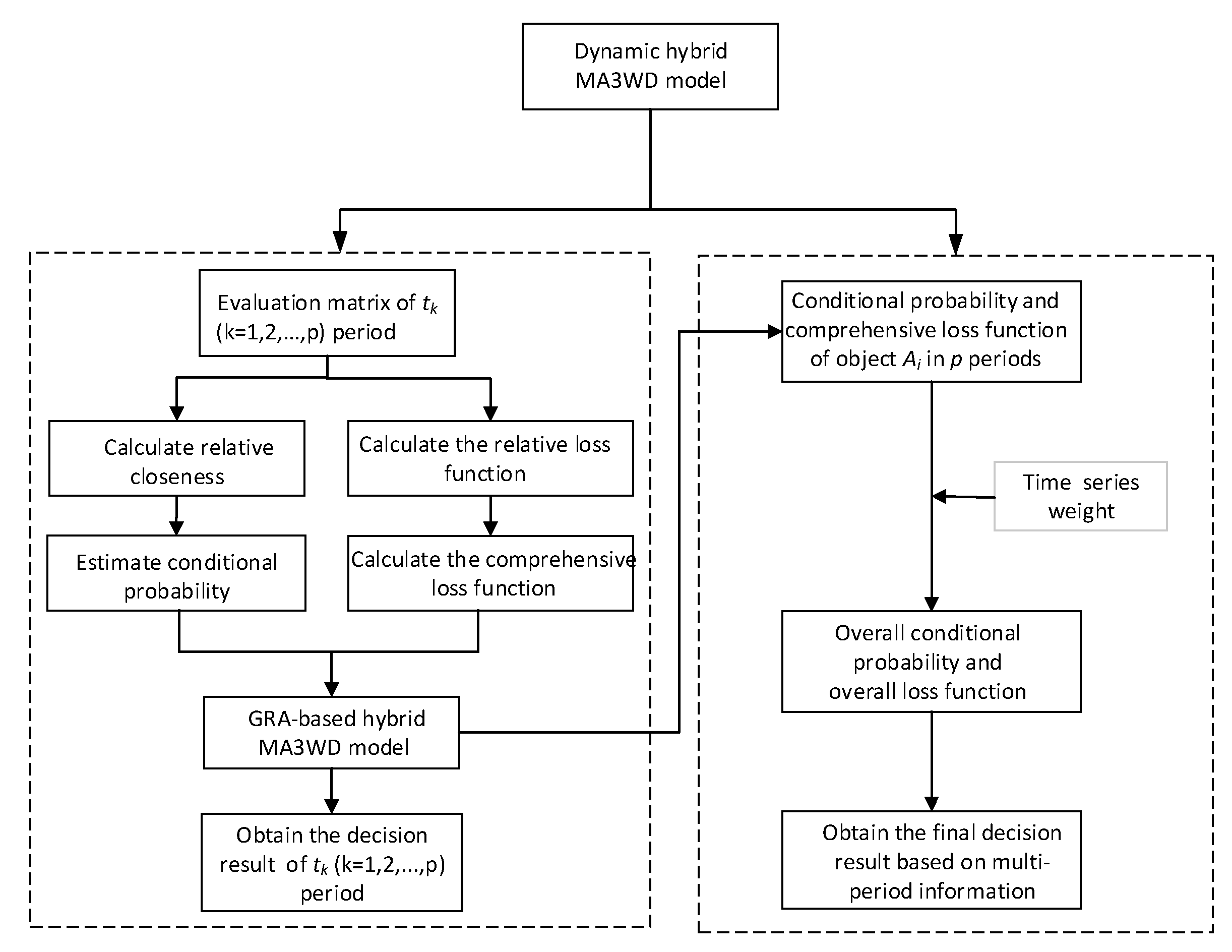
4. Dynamic Hybrid MA3WD Model for Multiple Periods

In this section, the calculation methods of weights for time series and attributes are discussed, respectively. Based on the GRA-based hybrid MA3WD model, a dynamic hybrid MA3WD model is then proposed by considering multi-period information. The specific process of the proposed model is shown in Figure 1.

4.1. Determination of Weights

(1)

Determination of time-series weights

An important feature of dynamic hybrid MA3WD is the time-series information, as data in different time series have different relative importance for final results. In this paper, the entropy-weight method is applied to obtain the weights of the time series. Nonlinear programming based on maximum entropy value is constructed to obtain the time-series weights as follows:

$$\begin{array}{l}\max I=-{\displaystyle \sum _{k=1}^p{\xi }^k\ln {\xi }^k}\\ st\left\{\begin{array}{l}{}_{}\lambda ={\displaystyle \sum _{k=1}^p\frac{p-k}{p-1}{\xi }^k}\\ {}_{}{\displaystyle \sum _{k=1}^p{\xi }^k=1}\\ {}_{}0\le {\xi }^k\le 1\\ {}_{}k=1,2,\dots ,p\end{array}\right.\end{array}$$

(32)

where ${\xi }^k$ is the weight of the $t_k$ period, and $p$ is the number of periods. $\lambda \in [0,1]$ means “time degree”, which reflects the importance of time series in the process of operator assembly. A value of $\lambda$ closer to 0 denotes that the decision-maker places more emphasis on recent data; a value of $\lambda$ closer to 1 denotes that the decision-maker places more emphasis on distant data. In addition, $\lambda =0.5$ denotes that the decision-maker places equal importance on each period and has no special preference [48].

(2)

Determination of attribute weights

To obtain the weights of attributes, a combination of BWM and entropy-weight methods is utilized. It avoids the excessive subjectivity in BWM, as well as the imbalance of indicator weights in the entropy-weight method. The specific steps of the BWM-entropy-weight method are described as follows.

Step 1. Obtain the subjective weights of attributes by BWM. BWM is a multi-criteria decision-making method proposed by Rezaei [49]. The method is based on the idea of pairwise comparison of indicators. First, the decision-makers select the optimal ${\mathrm{c}}_B$ and the worst from the evaluation indicators. Then, ${\mathrm{c}}_B$ and ${\mathrm{c}}_W$ are compared with other indicators to construct the comparison vectors of the optimal and worst indicators, which are, respectively, expressed as $A_B=\left(a_{B1},a_{B2},\dots ,a_{Bn}\right)$ and $A_W=\left(a_{1W},a_{2W},\dots ,a_{nW}\right)$ [50]. Next, the optimal weight values are obtained by constructing the following nonlinear programming model.

$$\begin{array}{l}\min \zeta \\ st\left\{\begin{array}{l}{}_{}\left|\frac{w_B}{w_j}-a_{Bj}\right|\le \zeta \\ {}_{}\left|\frac{w_j}{w_W}-a_{jW}\right|\le \zeta \\ {}_{}{\displaystyle \sum _{j=1}^n{w}_j=1}\\ {}_{}{w}_j\ge 0,j=1,2,\dots ,n\end{array}\right.\end{array}$$

(33)

In this paper, we consider the reality that a set of attributes expands over time. Therefore, when determining the attribute weights in different periods, we first use the BWM method ${\mathrm{c}}_W$ to calculate the weight of each attribute in the current period t_p that contains the most comprehensive attributes. Then, other periods are regarded as attribute subsets of the t_p period. For the acquisition of their attribute weights, we remove the attributes added in the t_p period and normalization, thus obtaining the attribute weight vector ${\tilde{W}}^k=\left({\tilde{w}}_1^k,{\tilde{w}}_2^k,\dots ,{\tilde{w}}_n^k\right)$ of the t_k (k = 1, 2, …, p) period based on the BWM method.

Step 2. Obtain the objective weights of attributes by the entropy-weight method. Entropy is a measure of system disorder in the entropy-weight method. In addition, the lower the entropy value of a set of values, the greater the change in data, and the greater the corresponding entropy weight [51]. The specific calculation steps of this method are

$$e_j=-\frac{1}{\ln m}{\displaystyle \sum _{i=1}^m\frac{D_{ij}}{D_j}}\ln \frac{D_{ij}}{D_j} (j=1,2,\dots ,n)$$

(34)

where $D_{ij}={\displaystyle \sum _{s=1}^{m}d\left(v_{ij},v_{sj}\right)}$ $(i=1,2,\dots ,m;j=1,2,\dots ,n)$ indicates the deviation of object $A_i$ from all other objects, and $D_j={\displaystyle \sum _{i=1}^m{D}_{ij}={\displaystyle \sum _{i=1}^m{\displaystyle \sum _{s=1}^{m}d\left(v_{ij},v_{sj}\right)}}}$ $(j=1,2,\dots ,n)$ indicates the deviation of all objects from other objects for attribute $c_j$. $d\left(v_{ij},v_{sj}\right)$ indicates the distance between $v_{ij}$ and $v_{sj}$. Then, the entropy weight $w_j$ of each attribute can be expressed as

$$w_j=\frac{1-e_j}{{\displaystyle \sum _{j=1}^n\left(1-e_j\right)}} (j=1,2,\dots ,n)$$

(35)

and then, we can obtain the attribute weight vector ${\stackrel{⌢}{W}}^k=\left({\stackrel{⌢}{w}}_1^k,{\stackrel{⌢}{w}}_2^k,\dots ,{\stackrel{⌢}{w}}_n^k\right)$ in the $t_k$ $(k=1,2,\dots ,p)$ period based on the entropy-weight method.

Step 3. Calculate the comprehensive weights of attributes. Through BWM and entropy-weight methods, the attribute weight vector of each period can be acquired, respectively. Then we combine the results of the two methods to obtain the attribute weight of the $t_k$$(k=1,2,\dots ,p)$ period as

$$w_j^k=\frac{{\tilde{w}}_j^k+{\stackrel{⌢}{w}}_j^k}{{\displaystyle \sum _{j=1}^n{\tilde{w}}_j^k+{\stackrel{⌢}{w}}_j^k}}$$

(36)

Then, we can obtain the comprehensive weight vector $W^k=\left(w_1^k,w_2^k,\dots ,w_n^k\right)$ in $t_k$$(k=1,2,\dots ,p)$.

4.2. Dynamic Hybrid MA3WD for Multiple Periods

In this section, a dynamic hybrid MA3WD model is established. First, a weighted average operator is employed to integrate the comprehensive loss functions of the alternative $A_i$ in each period $t_k$ shown in

Table 5. Comprehensive loss function of $A_i$ in the $t_k$ period.

${\mathit{A}}_{\mathit{i}}$	$\mathit{C}$	$\neg \mathit{C}$
$a_P$	0	${\displaystyle {\sum }_j{w}_j^k\left(1-r_{ij}^{k+}\right)}$
$a_B$	${\displaystyle {\sum }_j{w}_j^k{\sigma }_j^k\left(1-r_{ij}^{k-}\right)}$	${\displaystyle {\sum }_j{w}_j^k{\sigma }_j^k\left(1-r_{ij}^{k+}\right)}$
$a_N$	${\displaystyle {\sum }_j{w}_j^k\left(1-r_{ij}^{k+}\right)}$	0

, to obtain the overall loss function of the alternative $A_i$ as shown in

Table 6. Overall loss function of alternative $A_i$.

${\mathit{A}}_{\mathit{i}}$	$\mathit{C}$	$\neg \mathit{C}$
$a_P$	0	${\displaystyle {\sum }_k{\displaystyle {\sum }_j{\xi }^k{w}_j^k\left(1-r_{ij}^{k+}\right)}}$
$a_B$	${\displaystyle {\sum }_k{\displaystyle {\sum }_j{\xi }^k{w}_j^k{\sigma }_j^k\left(1-r_{ij}^{k-}\right)}}$	${\displaystyle {\sum }_k{\displaystyle {\sum }_j{\xi }^k{w}_j^k{\sigma }_j^k\left(1-r_{ij}^{k+}\right)}}$
$a_N$	${\displaystyle {\sum }_k{\displaystyle {\sum }_j{\xi }^k{w}_j^k\left(1-r_{ij}^{k-}\right)}}$	0

. Then, the overall conditional probability of the alternative $A_i$ is obtained in the same way. Finally, the three-way decision rules are established.

Table 6 shows that each loss ${\lambda }_{•\ast }$ ($•=P,B,N;\ast =P,N$) in the overall loss function is obtained by integrating the corresponding losses for $p$ periods. We calculate the thresholds according to the overall loss function, yielding:

$${\alpha }_i=\frac{{\displaystyle {\sum }_k{\displaystyle {\sum }_j{\xi }^k{w}_j^k\left(1-{\sigma }_j^k\right)\left(1-r_{ij}^{k+}\right)}}}{{\displaystyle {\sum }_k{\displaystyle {\sum }_j{\xi }^k{w}_j^k\left(1-{\sigma }_j^k\right)\left(1-r_{ij}^{k+}\right)}}+{\displaystyle {\sum }_k{\displaystyle {\sum }_j{\xi }^k{w}_j^k{\sigma }_j^k\left(1-r_{ij}^{k-}\right)}}}$$

(37)

$${\beta }_i=\frac{{\displaystyle {\sum }_k{\displaystyle {\sum }_j{\xi }^k{w}_j^k{\sigma }_j^k\left(1-r_{ij}^{k+}\right)}}}{{\displaystyle {\sum }_k{\displaystyle {\sum }_j{\xi }^k{w}_j^k{\sigma }_j^k\left(1-r_{ij}^{k+}\right)}}+{\displaystyle {\sum }_k{\displaystyle {\sum }_j{\xi }^k{w}_j^k\left(1-{\sigma }_j^k\right)\left(1-r_{ij}^{k-}\right)}}}$$

(38)

$${\gamma }_i=\frac{{\displaystyle {\sum }_k{\displaystyle {\sum }_j{\xi }^k{w}_j^k\left(1-r_{ij}^{k+}\right)}}}{{\displaystyle {\sum }_k{\displaystyle {\sum }_j{\xi }^k{w}_j^k\left(1-r_{ij}^{k+}\right)}}+{\displaystyle {\sum }_k{\displaystyle {\sum }_j{\xi }^k{w}_j^k\left(1-r_{ij}^{k-}\right)}}}$$

(39)

Through the process described in Section 3.2, we can calculate the conditional probability in each independent period ${\mathrm{Pr}}^k\left(C|[A_i]\right)$. Considering the information from multiple periods, the overall conditional probability $\mathrm{Pr}\left(C|[A_i]\right)$ of $A_i$ can be obtained by integrating the corresponding conditional probability ${\mathrm{Pr}}^k\left(C|[A_i]\right)$ for $k=1,2,\dots ,p$. We denote the overall conditional probability as

$$\mathrm{Pr}\left(C|[A_i]\right)={\displaystyle \sum _{k=1}^p{\xi }^k{\mathrm{Pr}}^k\left(C|[A_i]\right)}$$

(40)

Then, the three-way decision rules can be described as

$$(\mathrm{P})\mathrm{If}{\displaystyle \sum _{k=1}^p{\xi }^k{\mathrm{Pr}}^k\left(C|[A_i]\right)}\ge {\alpha }_i,\mathrm{decide}{A}_i\in POS(C);$$

$$(\mathrm{B})\mathrm{If}{\beta }_i<{\displaystyle \sum _{k=1}^p{\xi }^k{\mathrm{Pr}}^k\left(C|[A_i]\right)}<{\alpha }_i,\mathrm{decide}{A}_i\in BND(C);$$

$$(\mathrm{N})\mathrm{If}{\displaystyle \sum _{k=1}^p{\xi }^k{\mathrm{Pr}}^k\left(C|[A_i]\right)}\le {\beta }_i,\mathrm{decide}{A}_i\in NEG(C).$$

where ${\alpha }_i$ and ${\beta }_i$ are expressed as Equations (37) and (38). In the elderly-service performance evaluation application, if the object $A_i$ follows the rule (P), then $A_i\in POS(C)$, meaning the third-party organization has a good performance and is qualified to obtain a new contract with the government; if the object $A_i$ follows the rule (N), then $A_i\in NEG(C)$, meaning that the third-party organization has a poor performance and the government should terminate the contract with it; and if the object $A_i$ follows the rule (B), then $A_i\in BND(C)$, meaning that the third-party organization has a moderate performance and it should take self-inspection and self-rectification for further evaluation.

It should be noted that the third-party social organizations following rule (B) can locate their shortcomings to a certain period and certain attributes according to the proposed model because it also contains the evaluating results for each single period and each single attribute. Therefore, in the final result, the social organizations in the boundary region can determine the certain period in which they have poor performance. Similarly, they can also determine certain attributes with poor performance by the proposed model. Then they can rectify the corresponding shortcomings accurately and strive to establish a cooperative relationship with the government again in the next assessment.

4.3. The Key Steps and Algorithm of Dynamic Hybrid MA3WD Model

To illustrate the dynamic hybrid MA3WD model, we summarize the key steps as well as the Algorithm 1: The specific algorithm for dynamic hybrid MA3WD.of the proposed model.

Step 1. Calculate the relative loss function based on gray relational analysis in the $t_k$ ($k=1,2,\dots ,p$) period according to Table 4.

Step 2. Compute the comprehensive loss function of each object $A_i$ and the thresholds in $t_k$ period by Equations (29)–(31).

Step 3. Calculate the conditional probability ${\mathrm{Pr}}^k\left(C|[A_i]\right)$ through Section 3.2.

Step 4. Obtain the evaluation results of $A_i$ through the new GRA-based hybrid MA3WD model.

Step 5. Calculate the overall loss function and overall conditional probability based on the loss function and conditional probability obtained from the GRA-based hybrid MA3WD model.

Step 6. Obtain the final decision result of $A_i$ according to the three-way decision rules.

Algorithm 1: The specific algorithm for dynamic hybrid MA3WD.

Input: An information system $\left(T,U,C,V,f\right)$, the risk-avoidance coefficient vector ${\sigma }^k=\left({\sigma }_1^k,{\sigma }_2^k,\dots ,{\sigma }_n^k\right)$ for each period $t_k$, the attribute weight vector $W^k=\left(w_1^k,w_2^k,\dots ,w_n^k\right)$ for each period $t_k$, the time-series weight vector $\xi =\left({\xi }^1,{\xi }^2,\dots ,{\xi }^p\right)$. Output: The classification results of objects. Begin for k = 1 to p do  for $i=1$ to m and j=1 to n do  Calculate the relative loss function ${\lambda }_{•\ast }^{ijk}\left(•=P,B,N;\ast =P,N\right)$ according to Table 4.  end  for $i=1$ to m and j=1 to n do  Calculate the comprehensive loss function ${\lambda }_{•\ast }^{ijk}\left(•=P,B,N;\ast =P,N\right)$ by Equation (15).  end  for $i=1$ to m do  Calculate thresholds ${\alpha }_i^k$, ${\beta }_i^k$ and ${\gamma }_i^k$ by Equations (29)–(31).  end  for $i=1$ to m and j=1 to n do  Compute conditional probability ${\mathrm{Pr}}^k\left(C|[A_i]\right)$ according to Section 3.2.  for $i=1$ to m do  Determine the evaluation result of each object in the tk period in light of (${P^{\prime }}_{GRA}$)~(${N^{\prime }}_{GRA}$).  end end for $i=1$ to m and k=1 to p do  Calculate the overall loss function ${\lambda }_{•\ast }^i\left(•=P,B,N;\ast =P,N\right)$ according to Table 6. end for $i=1$ to m do  Calculate thresholds ${\alpha }_i$, ${\beta }_i$ and ${\gamma }_i$ by Equations (37)–(39). end for $i=1$ to m and k=1 to p do  Calculate the overall conditional probability $\mathrm{Pr}\left(C|[A_i]\right)$ by Equation (40). end for $i=1$ to m do  Obtain the final decision result of each object according to three-way decision rules. end

5. Case Illustration

5.1. Example Calculation

The demand for elderly care in China is rising with the acceleration of aging, and traditional elderly-care supply by governments cannot meet the practical requirements. Therefore, the government purchase of elderly-care services has been successfully adopted in China. We take Xinyang, a city in Henan Province, as an example. Given the obvious aging problem in the local area, the Xinyang government has actively invested special funds to purchase elderly-care services. Moreover, the government’s policy is to evaluate the elderly-care service performance of social organizations once every year and decide whether to renew the contract after three years. For this realistic requirement, the GRA-hybrid MA3WD model is used to evaluate the elderly-care service performance each year, and the dynamic hybrid MA3WD model is used to solve the renewal decision after three years.

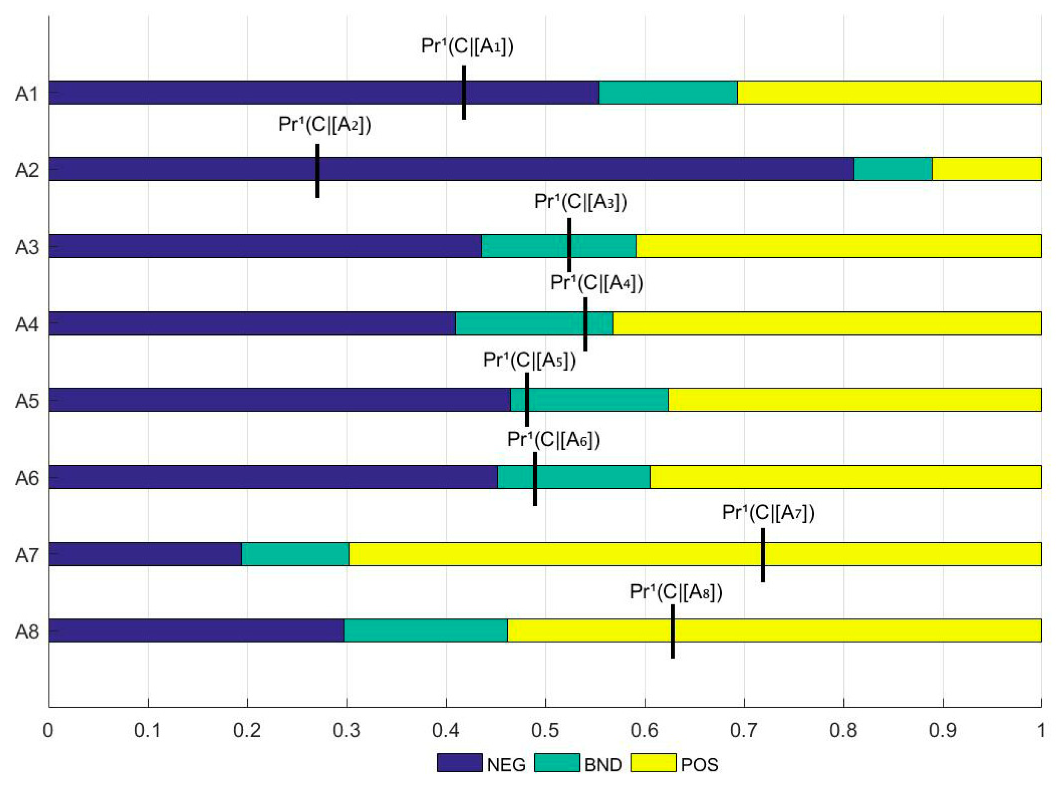
5.1.1. Evaluation Analysis for Single Period

There are eight social organizations $A_i$ ($i=1,2,\dots ,8$) that provide elderly-care services purchased by the government. As a period of three years comprises a decision-making cycle, the information of their latest three years (denoted as t₁, t₂, and t₃, respectively, where t₃ is the current period) is selected. For the t₁ and t₂ periods, the following evaluation indexes are used to evaluate the elderly-care services provided by social organizations [38,39].

① Professional training level ($c_1$). This attribute examines the standardization of training in social organizations and the degree of specialization of the trained personnel.

② Number of personalized service items ($c_2$). This attribute reflects the level of diversification of services provided by social organizations.

③ Information disclosure ($c_3$). This attribute examines the ability of social organizations to timely inform the elderly about service adjustment, to ensure the elderly’s right to know about services.

④ Timeliness of service ($c_4$). Timeliness refers to the swiftness and rapidness of time. The timeliness of providing elderly-care services means that elderly-care services can respond to the needs of service objects in time during the supply process.

⑤ Customer satisfaction ($c_5$). This attribute is the result of the continuous strengthening of customer satisfaction, reflecting the customer’s recognition, affirmation, and trust in the service.

⑥ Communication ability ($c_6$). This attribute is used to evaluate the ability of service personnel to communicate effectively with the elderly. With the extension of the service, social organizations provide psychological counseling and treatment to satisfy the needs of the elderly during the period t₃. Therefore, in the third year, decision-makers add a new evaluation attribute c₇.

⑦ Psychological treatment ability ($c_7$). Old people often have serious psychological problems such as the lack of company of family members and the fear of death, so social organizations need to provide psychological counseling and treatment.

To verify the feasibility of the method proposed in this paper, after a discussion among experts selected from the field of elderly-care services, the forms of different indexes are determined as shown in

Table 7. Classification of evaluation indexes.

Evaluation Indexes	Index Value Forms	Index Type
$c_1$	Triangular fuzzy numbers	Quantitative (benefit type)
$c_2$	Real numbers	Quantitative (benefit type)
$c_3$	Intuitionistic fuzzy numbers	Quantitative (benefit type)
$c_4$	Real numbers	Quantitative (benefit type)
$c_5$	Real numbers	Quantitative (benefit type)
$c_6$	Linguistic terms	Qualitative (benefit type)
$c_7$	Interval numbers	Quantitative (benefit type)

. During the discussion, experts determine the type of each index based on attribute characteristics as well as their own experience and preferences. For example, timeliness of service ($c_4$) and customer satisfaction ($c_5$) are best represented on a scale of 1–5 according to expert experience, with 5 indicating strong approval, 1 indicating complete disapproval, and intermediate scores indicating different degrees. Communication ability ($c_6$) is a qualitative index, so the linguistic variable is the most relevant tool. Furthermore, to demonstrate the applicability of the method to different information, experts were selected to rate based on their different preferences. The evaluation values of different social organizations in the three periods are shown in

Table 8. Decision matrix for the $t_1$ period.

	${\mathit{c}}_1$	${\mathit{c}}_2$	${\mathit{c}}_3$	${\mathit{c}}_4$	${\mathit{c}}_5$	${\mathit{c}}_6$
$A_1$	(0.64,0.7,0.76)	7	<0.8,0.1>	4	3	G
$A_2$	(0.6,0.68,0.76)	8	<0.75,0.15>	3	3	P
$A_3$	(0.7,0.75,0.8)	9	<0.85,0.1>	3	4	VG
$A_4$	(0.8,0.85,0.9)	8	<0.8,0.1>	4	3	VG
$A_5$	(0.72,0.8,0.88)	6	<0.85,0.1>	4	4	G
$A_6$	(0.65,0.7,0.75)	7	<0.8,0.1>	5	4	M
$A_7$	(0.81,0,85,0.89)	10	<0.8,0.1>	5	5	G
$A_8$	(0.75,0.85,0.95)	7	<0.75,0.15>	4	5	EG

,

Table 9. Decision matrix for the $t_2$ period.

	${\mathit{c}}_1$	${\mathit{c}}_2$	${\mathit{c}}_3$	${\mathit{c}}_4$	${\mathit{c}}_5$	${\mathit{c}}_6$
$A_1$	(0.68,0.72,0.76)	7	<0.8,0.1>	5	4	G
$A_2$	(0.65,0.70,0.75)	8	<0.75,0.15>	4	5	M
$A_3$	(0.8,0.85,0.9)	8	<0.85,0.1>	4	4	VG
$A_4$	(0.61,0.66,0.71)	8	<0.8,0.1>	3	3	G
$A_5$	(0.72,0.77,0.82)	6	<0.85,0.1>	4	5	VG
$A_6$	(0.75,0.8,0.85)	7	<0.8,0.1>	5	4	G
$A_7$	(0.82,0.87,0.91)	10	<0.8,0.1>	4	5	EG
$A_8$	(0.73,0.83,0.93)	9	<0.75,0.15>	4	5	EG

and

Table 10. Decision matrix for the $t_3$ period.

	${\mathit{c}}_1$	${\mathit{c}}_2$	${\mathit{c}}_3$	${\mathit{c}}_4$	${\mathit{c}}_5$	${\mathit{c}}_6$	${\mathit{c}}_7$
$A_1$	(0.68,0.73,0.78)	8	<0.8,0.1>	5	4	G	[77,81]
$A_2$	(0.7,0.75,0.8)	8	<0.75,0.15>	4	5	G	[77,81]
$A_3$	(0.74,0.79,0.84)	10	<0.85,0.1>	4	5	VG	[81,85]
$A_4$	(0.71,0.76,0.81)	9	<0.8,0.1>	3	3	G	[75,79]
$A_5$	(0.7,0.75,0.8)	8	<0.85,0.1>	5	5	VG	[81,85]
$A_6$	(0.8,0.84,0.9)	9	<0.8,0.1>	5	4	VG	[82,86]
$A_7$	(0.9,0.95,1)	10	<0.8,0.1>	4	5	EG	[86,90]
$A_8$	(0.65,0.7,0.75)	8	<0.75,0.15>	4	4	G	[75,79]

. In this case, experts use a 7-point linguistic term-set to evaluate $c_6$, denoted as

$$\begin{array}{l}T=\{t_0=extremly poor(EP),t_1=very poor(VP),t_2=poor(P),\\ \begin{array}{cc}& \end{array}{\hspace{1em}t}_3=medium(M),t_4=good(G),t_5=very good(VG),t_6=extremly good(EG)\}\end{array}$$

Considering that $c_3$ is not easy to change in the short term, the evaluation value of each object under this attribute is fixed in the three periods.

In the treatment of hybrid information, the distance between the hybrid information and the ideal solution is used as a basis for decision-making in this paper, to avoid information loss due to the interconversion of heterogeneous information [37]. The determination of ideal solution and distance of real numbers, interval numbers, triangular fuzzy numbers, and intuitionistic fuzzy numbers are, respectively, referred to [34,35,36,52], where for these basic concepts we do not elaborate too much. The linguistic term-set $T=\left\{t_k\right|k=1,2,\dots ,s\}$ is transformed into triangular fuzzy numbers to participate in the calculation, with the formula $\tilde{t}=(t_k^L,t_k^M,t_k^U)=(\max \{(k-1)/s,0\},k/s,$$\min \{(k+1)/s,1\}),k=1,2,\dots ,s$.

Considering the BWM and entropy-weight method, we can calculate the attribute weight vectors as $W^1=(0.211,0.162,0.129,0.192,0.132,0.175)$, $W^2=(0.222,0.146,0.106,0.255,0.155,0.115)$, and $W^3=(0.297,0.088,0.096,0.146,0.136,0.104,0.132)$ for $t_1$, $t_2$, and $t_3$ periods, respectively. According to the uncertain attitude of decision-makers towards different attributes, the risk-avoidance coefficient vector in the $t_1$ and $t_2$ periods is ${\sigma }^{1,2}=\left(0.35,0.45,0.35,0.4,0.4,0.5\right)$. As a new attribute is added in the $t_3$ period, the risk-avoidance coefficient vector of the period becomes ${\sigma }^3=\left(0.35,0.45,0.35,0.4,0.4,0.5,0.4\right)$. We follow the steps below to evaluate these eight social organizations (the calculation process of the $t_2$ or $t_3$ periods is the same as that of the $t_1$ period; we will not repeat the calculation steps, and only take the $t_1$ period as an example).

In the evaluation of third-party social organizations providing elderly-care services, there are two states $\mathsf{\Omega }=\{C,\neg C\}$, where $C$ denotes a good organization and $\neg C$ denotes a bad organization. Let the set of actions be represented as $A=\{a_P,a_B,a_N\}$, where $a_P$, $a_B$, and $a_N$ denote good performance, moderate performance, and poor performance, respectively. According to the discussion in Section 3, we first calculate the gray relational coefficients between the eight objects and PIS and NIS in the t₁ period by Equations (9) and (10). The relative loss functions of each evaluation value in the t₁ period are obtained as shown in

Table 11. Relative loss functions in the $t_1$ period.

		${\mathit{c}}_1$		${\mathit{c}}_2$		${\mathit{c}}_3$		${\mathit{c}}_4$		${\mathit{c}}_5$		${\mathit{c}}_6$
		${\mathit{C}}_1$	$\neg {\mathit{C}}_1$	${\mathit{C}}_2$	$\neg {\mathit{C}}_2$	${\mathit{C}}_3$	$\neg {\mathit{C}}_3$	${\mathit{C}}_4$	$\neg {\mathit{C}}_4$	${\mathit{C}}_5$	$\neg {\mathit{C}}_5$	${\mathit{C}}_6$	$\neg {\mathit{C}}_6$
A1	aP	0	0.448	0	0.493	0	0.103	0	0.394	0	0.565	0	0.484
	aB	0.043	0.157	0.110	0.222	0.049	0.036	0.157	0.157	0	0.226	0.260	0.242
	aN	0.124	0	0.245	0	0.140	0	0.394	0	0	0	0.520	0
A2	aP	0	0.468	0	0.394	0	0.204	0	0.565	0	0.565	0	0.667
	aB	0.032	0.164	0.177	0.177	0	0.077	0	0.226	0	0.226	0	0.333
	aN	0.092	0	0.394	0	0	0	0	0	0	0	0	0
A3	aP	0	0.394	0	0.245	0	0	0	0.565	0	0.394	0	0.306
	aB	0.081	0.138	0.222	0.110	0.071	0	0	0.226	0.157	0.157	0.309	0.153
	aN	0.233	0	0.493	0	0.204	0	0	0	0.394	0	0.619	0
A4	aP	0	0.245	0	0.394	0	0.103	0	0.394	0	0.565	0	0.306
	aB	0.135	0.086	0.177	0.177	0.049	0.036	0.157	0.157	0	0.226	0.309	0.153
	aN	0.386	0	0.394	0	0.140	0	0.394	0	0	0	0.619	0
A5	aP	0	0.330	0	0.565	0	0	0	0.394	0	0.394	0	0.484
	aB	0.112	0.116	0	0.254	0.071	0	0.157	0.157	0.157	0.157	0.260	0.242
	aN	0.320	0	0	0	0.204	0	0.394	0	0.394	0	0.520	0
A6	aP	0	0.448	0	0.493	0	0.103	0	0	0	0.394	0	0.594
	aB	0.043	0.157	0.110	0.222	0.049	0.036	0.226	0	0.157	0.157	0.176	0.297
	aN	0.124	0	0.245	0	0.140	0	0.565	0	0.394	0	0.351	0
A7	aP	0	0.246	0	0	0	0103	0	0	0	0	0	0.484
	aB	0.135	0.086	0.254	0	0.049	0.036	0.226	0	0.226	0	0.260	0.242
	aN	0.386	0	0.565	0	0.140	0	0.565	0	0.565	0	0.520	0
A8	aP	0	0.260	0	0.493	0	0.204	0	0.394	0	0	0	0
	aB	0.136	0.091	0.110	0.222	0	0.071	0.157	0.157	0.226	0	0.333	0
	aN	0.390	0	0.245	0	0	0	0.394	0	0.565	0	0.667	0

. Then, we use the attribute weight vector $W^1$ to aggregate the relative loss functions to obtain the comprehensive loss functions of each object as shown in

Table 12. Comprehensive loss functions in the $t_1$ period.

		$\mathit{C}$	$\neg \mathit{C}$			$\mathit{C}$	$\neg \mathit{C}$
A1	aP	0	0.423	A5	aP	0	0.373
	aB	0.109	0.176		aB	0.129	0.159
	aN	0.250	0		aN	0.312	0
A2	aP	0	0.489	A6	aP	0	0.344
	aB	0.035	0.204		aB	0.128	0.146
	aN	0.083	0		aN	0.306	0
A3	aP	0	0.337	A7	aP	0	0.150
	aB	0.137	0.138		aB	0.195	0.065
	aN	0.316	0		aN	0.465	0
A4	aP	0	0.333	A8	aP	0	0.237
	aB	0.148	0.138		aB	0.165	0.095
	aN	0.347	0		aN	0.389	0

. Next, we can calculate the conditional probability of each object using the GRA-TOPSIS method mentioned in Section 3.2. Meanwhile, the thresholds of each object can be obtained by Equations (29)–(31). The thresholds and conditional probabilities are listed in

Table 13. Decision thresholds and conditional probabilities in the $t_1$ period.

	A1	A2	A3	A4	A5	A6	A7	A8
${\alpha }_i^1$	0.693	0.889	0.592	0.568	0.624	0.606	0.303	0.463
${\beta }_i^1$	0.555	0.881	0.436	0.410	0.465	0.452	0.194	0.297
${\gamma }_i^1$	0.628	0.855	0.516	0.489	0.545	0.529	0.244	0.378
${\mathrm{Pr}}^1\left(C|\left[A_i\right]\right)$	0.417	0.268	0.523	0.545	0.482	0.488	0.717	0.632

.

For each object, the range of each region and the conditional probability are shown in Figure 2. The region where ${\mathrm{Pr}}^1(C|[A_i])$ falls represents the decision of $A_i$ in the $t_1$ period, so we can obtain three-way decision results clearly from Figure 2 as: $POS(C)=\{A_7,A_8\}$, $BND(C)=\{A_3,A_4,A_5,A_6\}$ and $NEG(C)=\{A_1,A_2\}$. From the results, in the $t_1$ period, social organizations $A_7$ and $A_8$ are divided into the positive region, indicating that these two meet the standard of eligibility; $A_3$, $A_4$, $A_5$ and $A_6$ are divided into the boundary region, meaning that they perform moderately and should strive to improve their business in the next period; $A_1$ and $A_2$ are divided into the negative region, indicating these two perform poorly and may face the risk of elimination in the final decision if they do not make a change.

As the calculation process of $t_2$ and $t_3$ is the same as $t_1$, the calculation results of $t_2$ and $t_3$ are directly given, which are listed in

Table 14. Decision thresholds and conditional probabilities in the $t_2$ and $t_3$ periods.

		A1	A2	A3	A4	A5	A6	A7	A8
$t_2$	${\alpha }_i^2$	0.531	0.600	0.517	0.800	0.550	0.491	0.332	0.426
	${\beta }_i^2$	0.360	0.427	0.344	0.688	0.371	0.325	0.179	0.253
	${\gamma }_i^2$	0.444	0.514	0.428	0.750	0.459	0.404	0.250	0.336
	${\mathrm{Pr}}^2\left(C|\left[A_i\right]\right)$	0.543	0.483	0.567	0.311	0.536	0.575	0.694	0.643
$t_3$	${\alpha }_i^3$	0.593	0.601	0.452	0.752	0.448	0.437	0.184	0.699
	${\beta }_i^3$	0.405	0.413	0.268	0.592	0.269	0.261	0.090	0.529
	${\gamma }_i^3$	0.500	0.508	0.356	0.679	0.355	0.344	0.130	0.620
	${\mathrm{Pr}}^3\left(C|\left[A_i\right]\right)$	0.461	0.458	0.577	0.330	0.575	0.594	0.709	0.371

.

From the 3WD results of

Table 15. Three-way decision results in $t_2$ and $t_3$ periods.

	POS(C)	BND(C)	NEG(C)
$t_2$	$\{A_1,A_3,A_6,A_7,A_8\}$	$\{A_2,A_5\}$	$\left\{A_4\right\}$
$t_3$	$\{A_3,A_5,A_6,A_7\}$	$\{A_1,A_2\}$	$\{A_4,A_8\}$

, we can observe the different results of the $t_2$ and $t_3$ periods. In the $t_2$ period, social organizations $A_1$, $A_3$, $A_6$, $A_7$, and $A_8$ are classified into the positive region, meaning that the five objects perform well; $A_4$ is classified into the negative region, indicating poor performance during this period; $A_2$ and $A_5$ are classified into the boundary region, which means they have mediocre performance and need further improvement to reach the standard of renewal. Similarly, in the $t_3$ period, social organizations $A_3$, $A_5$, $A_6$, and $A_7$ perform well; $A_4$ and $A_8$ perform poorly; and $A_1$ and $A_2$ perform mediocrely, and need to work hard to improve business.

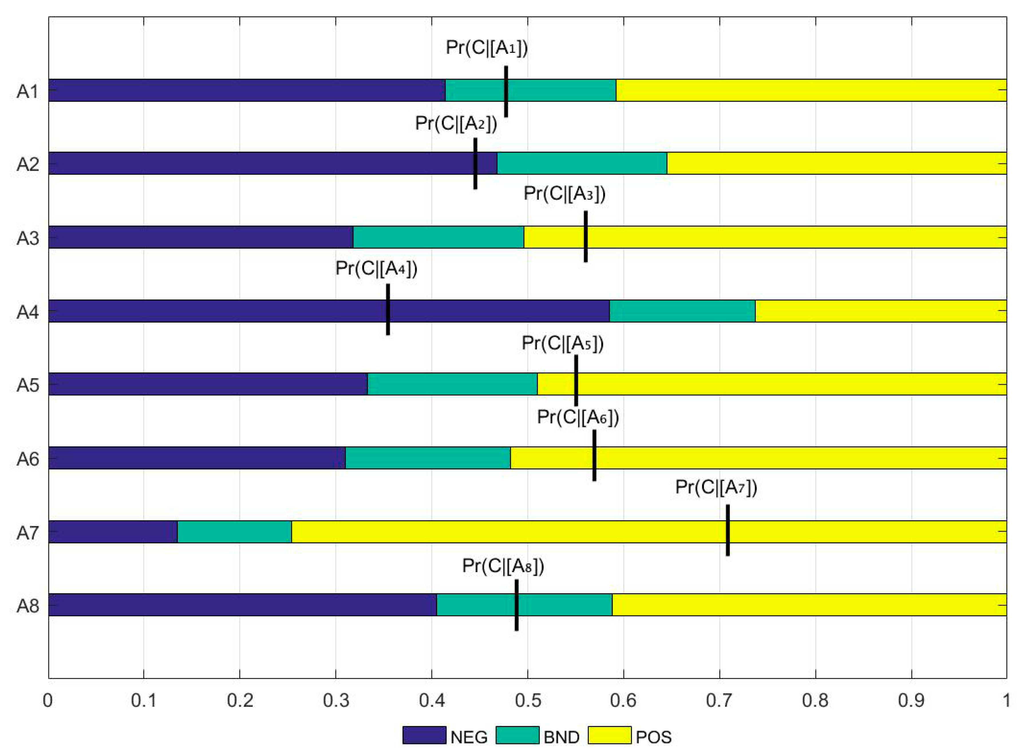
5.1.2. Decision Analysis for Multiple Periods

According to the process of the GRA-based hybrid MA3WD model, the corresponding comprehensive loss function and the conditional probability of each object of the three periods are obtained in Section 5.1.1. Since the decision-maker attaches more importance to the recent data, the value of the time degree $\lambda$ is set to 0.3, and then the time-series weight vector is obtained according to Equation (32) as follows: $\xi =(0.154,0.292,0.554)$. Next, use the time-series weights to integrate the comprehensive loss functions of the $t_1$, $t_2$ and $t_3$ periods to obtain the overall loss functions as shown in

Table 16. Overall loss functions.

		$\mathit{C}$	$\neg \mathit{C}$			$\mathit{C}$	$\neg \mathit{C}$
A1	aP	0	0.319	A5	aP	0	0.256
	aB	0.130	0.130		aB	0.146	0.105
	aN	0.314	0		aN	0.355	0
A2	aP	0	0.348	A6	aP	0	0.246
	aB	0.114	0.142		aB	0.156	0.101
	aN	0.274	0		aN	0.382	0
A3	aP	0	0.257	A7	aP	0	0.105
	aB	0.156	0.103		aB	0.186	0.042
	aN	0.378	0		aN	0.454	0
A4	aP	0	0.403	A8	aP	0	0.313
	aB	0.086	0.163		aB	0.132	0.124
	aN	0.201	0		aN	0.314	0

. It should be noted that the meaning of the actions set $A=\{a_P,a_B,a_N\}$ in Table 16 is slightly different from that mentioned in Section 5.1.1. Here, $a_P$, $a_B$ and $a_N$ denote the renewal of contract, further investigation, and termination of contract, respectively. Like the method used to calculate the overall loss functions, we integrate the corresponding conditional probability of each object in three periods to obtain the overall conditional probability $\mathrm{Pr}(C|[A_i])$ of each object. The thresholds and overall conditional probabilities are listed in

Table 17. Decision thresholds and overall conditional probabilities.

	A1	A2	A3	A4	A5	A6	A7	A8
${\alpha }_i$	0.592	0.645	0.496	0.737	0.511	0.482	0.254	0.588
${\beta }_i$	0.414	0.468	0.318	0.585	0.333	0.310	0.135	0.405
${\gamma }_i$	0.504	0.559	0.405	0.667	0.419	0.392	0.188	0.499
$\mathrm{Pr}\left(C|\left[A_i\right]\right)$	0.478	0.436	0.566	0.357	0.549	0.572	0.705	0.491

.

From Figure 3, we can visually observe the final 3WD results after comprehensively considering the evaluation information of three periods. Now, according to the classification results, the government can decide on which social organizations to continue to cooperate with. As shown in Figure 3, $POS(C)=\{A_3,A_5,A_6,A_7\}$, $BND(C)=\{A_1,A_8\}$ and $NEG(C)=\{A_2,A_4\}$. Therefore, social organizations $A_3$, $A_5$, $A_6$, and $A_7$ have good performances and are qualified to obtain new contracts with the government; $A_2$ and $A_4$ have poor performances and government should terminate contracts with them; $A_1$ and $A_8$ have moderate performances and they should take self-inspection and self-rectification for further evaluation.

As mentioned in Section 4, the model proposed in this paper can precisely locate which attributes are underperforming at which period for the social organization, to rectify and manage the corresponding business. Hence, for the social organizations in the boundary region, they can make targeted rectifications according to the results of the model, and perform outstandingly in the next assessment. For example, in the final decision results, $A_8$ is divided into the boundary region. According to Table 13 and Table 15, $A_8$ is divided into the positive region, while in the $t_3$ period, it is divided into the negative region. Based on this situation, for $A_8$, we can explore which attributes underperform at $t_3$, i.e., which attributes are divided into the negative region. Considering a single attribute as a 3WD problem, the 3WD rules of A₈ under each attribute are obtained based on the 3WD method proposed in this paper.

According to the thresholds and conditional probabilities listed in

Table 18. Calculation results of A₈ under each attribute.

		${\mathit{c}}_1$	${\mathit{c}}_2$	${\mathit{c}}_3$	${\mathit{c}}_4$	${\mathit{c}}_5$	${\mathit{c}}_6$	${\mathit{c}}_7$
$A_8$	$\alpha$	0.870	0.550	1	0.6	0.6	0.482	1
	$\beta$	0.661	0.450	1	0.4	0.4	0.482	1
	$\mathrm{Pr}(C_j|[A_8])$	0.259	0.356	0.285	0.5	0.5	0.346	0.264

, we can judge that A₈ is classified into the rejection region under attributes $c_1$, $c_2$, $c_3$, $c_6$, and $c_7$, which means $A_8$ performs worse in these five attributes. From this result, if $A_8$ wants to improve its service performance, it should rectify the business related to these five attributes.

5.2. Comparative Analysis

5.2.1. Comparison between Static and Dynamic Assessment

To illustrate the importance of dynamic evaluation, we compare the results of the 3WD based on the evaluation information in the $t_3$ (current) period with the results of the 3WD based on the comprehensive information, i.e., when $t=t_3$ and $t=t_1\sim t_3$. The comparison results are shown in

Table 19. Comparison at t = t₃ and t = t₁ ~ t₃.

	POS(C)	BND(C)	NEG(C)
$t=t_3$	$\{A_3,A_5,A_6,A_7\}$	$\{A_1,A_2\}$	$\{A_4,A_8\}$
$t=t_1\sim t_3$	$\{A_3,A_5,A_6,A_7\}$	$\{A_1,A_8\}$	$\{A_2,A_4\}$

.

From Table 19, it can be seen that there are differences in the results derived from static and dynamic assessment. However, the result based on dynamic assessment is more reasonable. For example, in the $t_3$ period, $A_8$ is divided into the negative region, but if the evaluation information of the $t_1\sim t_3$ periods is considered, $A_8$ is classified in the boundary region. By comparing the decision results of $t_1$ and $t_2$, we can find that $A_8$ performs well in the first two periods and is classified into the positive region. This suggests that $A_8$ only performs poorly in the $t_3$ period, but still has the potential to be renewed and should be given a chance to rectify for the next assessment. Based on the above discussion, integrating multiple periods leads to more credible classification results, which demonstrates the importance of dynamic assessment.

5.2.2. Comparison between the Proposed Method and MADM Methods

In the current section, we compare the proposed method with three traditional MADM methods (the TOPSIS method [53], the VIKOR method [54], and the ELECTRE method [55]). It should be noted that the 3WD method is about the classification of alternatives, while these three MADM methods are only for obtaining the ranking of alternatives and determining an optimal alternative. To compare with these three MADM methods, the ranking of the alternatives is obtained according to the thresholds $\alpha$, $\beta$, and $\gamma$, respectively. The smaller the value of $\alpha$ (or $\beta$ or $\gamma$) of the alternative, the higher the probability of the alternative being accepted [20], so we obtain three sorting results according to the values of $\alpha$, $\beta$, and $\gamma$, which are shown in

Table 20. Ranking comparison of alternatives obtained by different methods.

	Proposed Method (Based on $\mathit{\alpha }$)	Proposed Method (Based on $\mathit{\beta }$)	Proposed Method (Based on $\mathit{\gamma }$)	TOPSIS [53]	VIKOR [54]	ELECTRE [55]
A1	6	6	6	6	6	6
A2	7	7	7	7	8	7
A3	3	3	3	4	3	4
A4	8	8	8	8	7	8
A5	4	4	4	3	4	2
A6	2	2	2	2	2	3
A7	1	1	1	1	1	1
A8	5	5	5	5	5	5

.

From Table 20, it can be seen that the ranking results of different methods are highly consistent, although there are slight differences. More specifically, there is a difference in the sorting of $A_3$, $A_5$, and $A_6$ for all methods, which indicates that the proposed method is valid. In addition, compared with the MADM method, the method proposed in this paper considers the risk preference of the decision-maker and divides all social organizations into three areas, which effectively reduces decision-making risks and helps the decision-maker make the most reasonable decision.

5.2.3. Comparison between the Proposed Method and Existing 3WD Methods

To further illustrate the superiority of the proposed model, we select Jia and Liu’s method [20], Gao et al.’s method [13], and Wang et al.’s method [56] for comparison. These three methods are first applied to the example in this section to obtain the classification results, which are listed in

Table 21. Comparison of classification results.

	POS(C)	BND(C)	NEG(C)
Jia and Liu’s method [20]	$\left\{A_3,A_5,A_6,A_7\right\}$	$\left\{A_1,A_8\right\}$	$\left\{A_2,A_4\right\}$
Gao et al.’s method [13]	$\left\{A_3,A_5,A_6,A_7\right\}$	$\varnothing$	$\left\{A_1,A_2,A_4,A_8\right\}$
Wang et al.’s method [56]	$\left\{A_3,A_5,A_6,A_7\right\}$	$\left\{A_1,A_8\right\}$	$\left\{A_2,A_4\right\}$
Proposed method	$\left\{A_3,A_5,A_6,A_7\right\}$	$\left\{A_1,A_8\right\}$	$\left\{A_2,A_4\right\}$

. Then, we compare and analyze the similarities and differences between the proposed method and the above methods considering four aspects, which are listed in

Table 22. Comparative analysis among different methods.

Different Methods	Attribute Weights	Outcome or Loss Functions	Conditional Probability	Dynamic Decision-Making
Jia and Liu’s method [20]	Subjective	Objective	Subjective	×
Gao et al.’s method [13]	Objective	Objective	Objective	√
Wang et al.’s method [56]	Subjective	Subjective	Objective	×
Proposed method	Objective	Objective	Objective	√

.

As shown in Table 21, the classification results of the four methods are generally consistent. $A_3$, $A_5$, $A_6$, and $A_7$ are all classified into the accept region, $A_2$ and $A_4$ are both classified into the reject region. There are only differences as to whether $A_1$ and $A_8$ are classified in the boundary region or the negative region. Based on the comparison of classification results, the effectiveness of our proposed method can be verified. Next, through the comparison in Table 22, we summarize the advantages of the method proposed in this paper:

(1)

Jia and Liu [20] converted attribute values into loss functions using relative loss and inverse loss functions, which is a great advance on the 3WD model. The determination of conditional probabilities is subjectively given by the decision-maker and lacks interpretability. The method proposed in this paper uses GRA-TOPSIS to estimate conditional probabilities, which overcomes the subjective influence of conditional probabilities given artificially.

(2)

Gao et al.’s method [13] considers the influence of time factors on realistic decision problems and considers the integration of information from multiple periods to make decisions. In some decision-making problems, it is also necessary to evaluate objects in a certain period. Gao et al. [13] lack the evaluation of objects in a single period. In contrast, the model proposed in this paper not only obtains the final decision results but also obtains the results of a certain period and a certain attribute, which facilitates the object to accurately determine which attribute is at a disadvantage for rectification. From this perspective, the proposed model is superior because of its flexibility and universality in the presentation of results.

(3)

Wang et al.’s method [56] introduces regret theory into the 3WD process, which is a great improvement to the 3WD and provides a guiding direction for our future research work. However, both the attribute weights and outcome matrix are decided subjectively by the decision-maker, which lacks transparency and interpretability. The method proposed in this paper uses a combination of BWM and entropy-weight methods to determine the attribute weights, which is more scientific than the method of Wang et al. [56]. At the same time, the proposed model uses GRA to construct the loss functions, which effectively connects the attribute values in the MADM with the loss functions in the 3WD from an objective perspective.

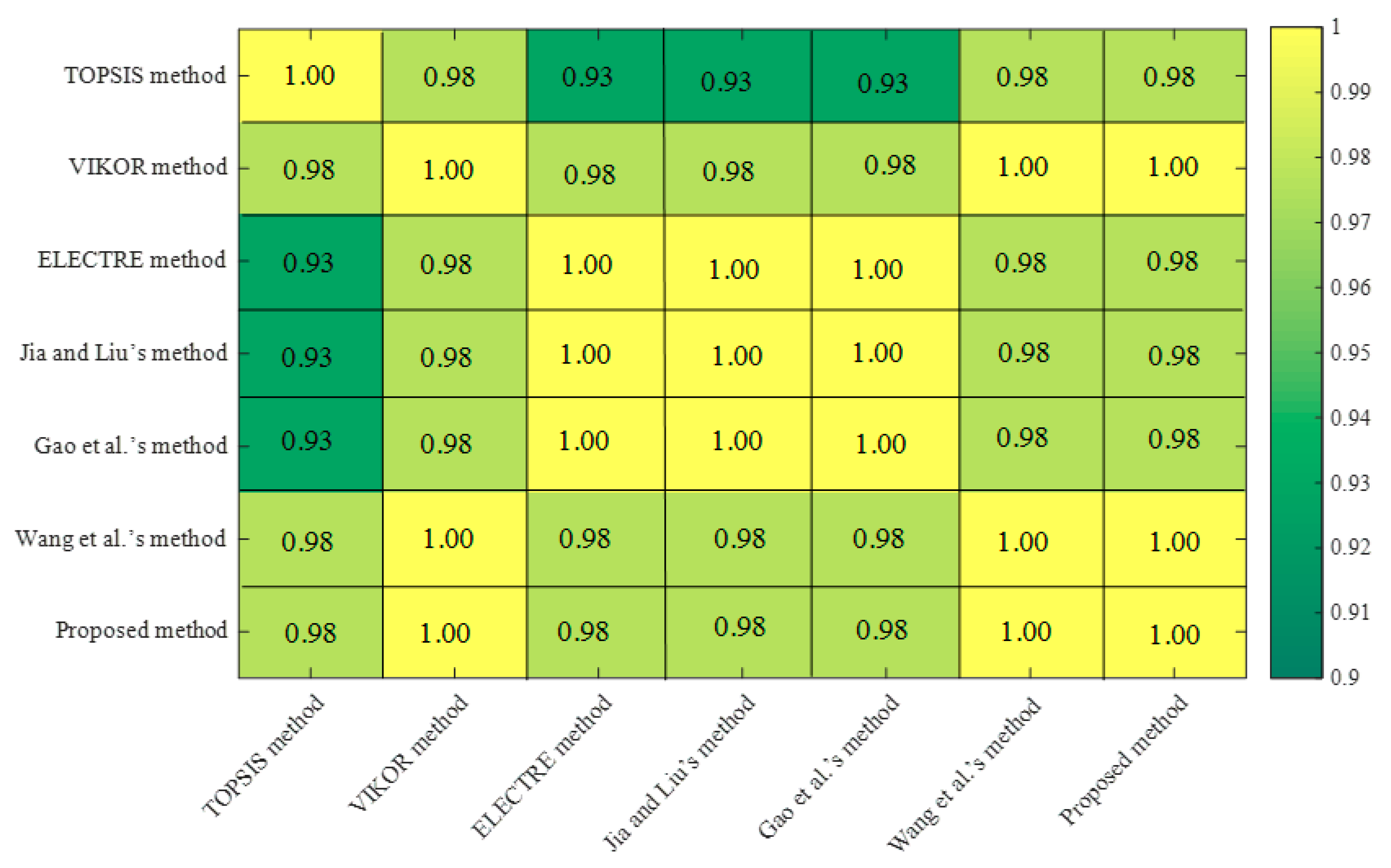
5.2.4. Correlation Analysis

In this section, we introduce the pairwise comparison method Spearman’s correlation coefficient (SCC) [57] to explore the connection of the above methods. There is a consensus that a larger SCC indicates a stronger consistency between the two methods. In general, an SCC greater than 0.8 indicates a strong correlation between the two counterparts. The specific calculation results are shown in Figure 4.

The results in Figure 4 show that all the SCCs between the proposed method and the other selected methods are greater than 0.9; therefore, there is a conclusion that the results derived from the proposed method are valid and credible.

6. Conclusions

In this paper, a GRA-based dynamic hybrid MA3WD model is established, and the main contributions of the method are listed as follows: (1) a new loss function construction method is proposed based on GRA, which adopts a data-driven method to overcome the drawback of excessive subjectivity caused by decision-makers giving loss functions based on experience; (2) with the aid of GRA-TOPSIS method, a new conditional probability determination method is proposed, which is based on the relative closeness reflecting the position and shape similarity; (3) a GRA-based hybrid MA3WD model is proposed for evaluating objects at a specific period. The model can point out the specific attributes and periods of poor performance of the object, which facilitates the object to improve its deficiencies accurately; (4) by extending the single-period environment to a multi-period environment, a dynamic hybrid MA3WD model is proposed, which extends the study of 3WD in a time-dynamic environment.

The proposed model is applied to solve the performance evaluation problem of elderly-care services to illustrate the feasibility and superiority of the proposed method, and the applicability of the proposed method is as follows: (1) the model applies to realistic problems with hybrid information derived from single-period evaluation information as well as multi-period information, which is widely applicable and flexible; (2) the proposed model can be used not only in the performance evaluation of elderly-care services but also in similar decision-making problems in other fields, such as target–threat assessment [13], investment decisions [30], risk analysis [58], medical diagnosis [28], etc.

There are some limitations, namely: (1) some existing 3WD methods have considered the psychological behavior of decision-makers [25], which is not mentioned in this paper, and the proposed method can be combined with regret theory [21] in future work; (2) in the dynamic MA3WD model, we calculate the time-series weights based on the entropy-weight method. Although this method is classical, it can be improved to obtain more reasonable time-series weights. Therefore, we will focus on three aspects in future studies: (1) the proposed method should be combined with group decision-making [59] to make the evaluation information used in decision-making more accurate and reliable; (2) considering the advantages of machine learning, we will introduce the knowledge of machine learning [60] in future studies on 3WD; (3) based on the characteristic that decision-makers are rational, we will consider combining the proposed method with behavioral decision theories such as regret theory [21] and prospect theory [61].

References

1. Rawat, S.S.; Pant, S.; Kumar, A.; Ram, M.; Sharma, H.K.; Kumar, A. A state-of-the-art survey on analytical hierarchy process applications in sustainable development. Sciences 2022, 7, 883–917. [Google Scholar] [CrossRef]
2. Rouyendegh, B.D.; Topuz, K.; Dag, A.; Oztekin, A. An AHP-IFT Integrated Model for Performance Evaluation of E-Commerce Web Sites. Inf. Syst. Front. 2019, 21, 1345–1355. [Google Scholar] [CrossRef]
3. Liu, P.D.; Shen, M.J. Failure Mode and Effects Analysis (FMEA) for Traffic Risk Assessment Based on Unbalanced Double Hierarchy Linguistic Term Set. Int. J. Fuzzy Syst. 2022, 25, 423–450. [Google Scholar] [CrossRef]
4. Wu, J.; Gong, H.; Liu, F.; Liu, Y. Risk Assessment of Open-Pit Slope Based on Large-Scale Group Decision-Making Method Considering Non-Cooperative Behavior. Int. J. Fuzzy Syst. 2023, 25, 245–263. [Google Scholar] [CrossRef]
5. Wang, Z.; Xiao, F.Y.; Ding, W.P. Interval-valued intuitionistic fuzzy jenson-shannon divergence and its application in multi-attribute decision making. Appl. Intell. 2022, 52, 16168–16184. [Google Scholar] [CrossRef]
6. Jiang, H.B.; Zhan, J.M.; Sun, B.Z.; Alcantud, J.C.R. An MADM approach to covering-based variable precision fuzzy rough sets: An application to medical diagnosis. Int. J. Mach. Learn. Cybern. 2020, 11, 2181–2207. [Google Scholar] [CrossRef]
7. Zhang, L.H.; Zhao, Z.L.; Yang, M.; Li, S.R. A multi-criteria decision method for performance evaluation of public charging service quality. Energy 2020, 195, 116958. [Google Scholar] [CrossRef]
8. dos Santos, B.M.; Godoy, L.P.; Campos, L.M.S. Performance evaluation of green suppliers using entropy-TOPSIS-F. J. Clean. Prod. 2019, 207, 498–509. [Google Scholar] [CrossRef]
9. Gong, J.W.; Liu, H.C.; You, X.Y.; Yin, L.S. An integrated multi-criteria decision making approach with linguistic hesitant fuzzy sets for E-learning website evaluation and selection. Appl. Soft Comput. 2021, 102, 107118. [Google Scholar] [CrossRef]
10. Luo, S.Z.; Liang, W.Z. A hybrid TODIM approach with unknown weight information for the performance evaluation of cleaner production. Comput. Appl. Math. 2021, 40, 23. [Google Scholar] [CrossRef]
11. Lam, W.S.; Lam, W.H.; Jaaman, S.H.; Liew, K.F. Performance Evaluation of Construction Companies Using Integrated Entropy-Fuzzy VIKOR Model. Entropy 2021, 23, 320. [Google Scholar] [CrossRef] [PubMed]
12. Lu, M.T.; Hsu, C.C.; Liou, J.J.H.; Lo, H.W. A hybrid MCDM and sustainability-balanced scorecard model to establish sustainable performance evaluation for international airports. J. Air Transp. Manag. 2018, 71, 9–19. [Google Scholar] [CrossRef]
13. Gao, Y.; Li, D.S.; Zhong, H. A novel target threat assessment method based on three-way decisions under intuitionistic fuzzy multi-attribute decision making environment. Eng. Appl. Artif. Intell. 2020, 87, 103276. [Google Scholar] [CrossRef]
14. Jiang, H.B.; Hu, B.Q. A decision-theoretic fuzzy rough set in hesitant fuzzy information systems and its application in multi-attribute decision-making. Inf. Sci. 2021, 579, 103–127. [Google Scholar] [CrossRef]
15. Yao, Y.Y. Three-way decisions with probabilistic rough sets. Inf. Sci. 2010, 180, 341–353. [Google Scholar] [CrossRef] [Green Version]
16. Yao, Y.Y. The superiority of three-way decisions in probabilistic rough set models. Inf. Sci. 2011, 181, 1080–1096. [Google Scholar] [CrossRef]
17. Li, H.X.; Zhang, L.B.; Huang, B.; Zhou, X.Z. Sequential three-way decision and granulation for cost-sensitive face recognition. Knowl.-Based Syst. 2016, 91, 241–251. [Google Scholar] [CrossRef]
18. Mandal, P.; Ranadive, A.S. Multi-granulation fuzzy probabilistic rough sets and their corresponding three-way decisions over two universes. Iran. J. Fuzzy Syst. 2019, 16, 61–76. [Google Scholar] [CrossRef]
19. Xu, Y.; Tang, J.X.; Wang, X.S. Three sequential multi-class three-way decision models. Inf. Sci. 2020, 537, 62–90. [Google Scholar] [CrossRef]
20. Jia, F.; Liu, P.D. A novel three-way decision model under multiple-criteria environment. Inf. Sci. 2019, 471, 29–51. [Google Scholar] [CrossRef]
21. Zhu, J.X.; Ma, X.L.; Zhan, J.M. A regret theory-based three-way decision approach with three strategies. Inf. Sci. 2022, 595, 89–118. [Google Scholar] [CrossRef]
22. Zhan, J.M.; Ye, J.; Ding, W.P.; Liu, P.D. A Novel Three-Way Decision Model Based on Utility Theory in Incomplete Fuzzy Decision Systems. IEEE Trans. Fuzzy Syst. 2022, 30, 2210–2226. [Google Scholar] [CrossRef]
23. Zhan, J.M.; Jiang, H.B.; Yao, Y.Y. Three-Way Multiattribute Decision-Making Based on Outranking Relations. IEEE Trans. Fuzzy Syst. 2021, 29, 2844–2858. [Google Scholar] [CrossRef]
24. Huang, X.F.; Zhan, J.M.; Sun, B.Z. A three-way decision method with pre-order relations. Inf. Sci. 2022, 595, 231–256. [Google Scholar] [CrossRef]
25. He, S.F.; Wang, Y.M.; Pan, X.H.; Chin, K.S. A novel behavioral three-way decision model with application to the treatment of mild symptoms of COVID-19. Appl. Soft Comput. 2022, 124, 109055. [Google Scholar] [CrossRef]
26. Sun, B.Z.; Chen, X.T.; Zhang, L.Y.; Ma, W.M. Three-way decision making approach to conflict analysis and resolution using probabilistic rough set over two universes. Inf. Sci. 2020, 507, 809–822. [Google Scholar] [CrossRef]
27. Yao, Y.Y. Three-way conflict analysis: Reformulations and extensions of the Pawlak model. Knowl.-Based Syst. 2019, 180, 26–37. [Google Scholar] [CrossRef]
28. Chen, Y.F.; Yue, X.D.; Fujita, H.; Fu, S.Y. Three-way decision support for diagnosis on focal liver lesions. Knowl.-Based Syst. 2017, 127, 85–99. [Google Scholar] [CrossRef]
29. Li, Z.W.; Xie, N.X.; Huang, D.; Zhang, G.Q. A three-way decision method in a hybrid decision information system and its application in medical diagnosis. Artif. Intell. Rev. 2020, 53, 4707–4736. [Google Scholar] [CrossRef]
30. Jiang, H.B.; Hu, B.Q. A novel three-way group investment decision model under intuitionistic fuzzy multi-attribute group decision-making environment. Inf. Sci. 2021, 569, 557–581. [Google Scholar] [CrossRef]
31. Li, X.; Huang, X.J. A Novel Three-Way Investment Decisions Based on Decision-Theoretic Rough Sets with Hesitant Fuzzy Information. Int. J. Fuzzy Syst. 2020, 22, 2708–2719. [Google Scholar] [CrossRef]
32. Zhi, H.L.; Qi, J.J.; Qian, T.; Wei, L. Three-way dual concept analysis. Int. J. Approx. Reason. 2019, 114, 151–165. [Google Scholar] [CrossRef]
33. He, X.L.; Wei, L.; She, Y.H. L-fuzzy concept analysis for three-way decisions: Basic definitions and fuzzy inference mechanisms. Int. J. Mach. Learn. Cybern. 2018, 9, 1857–1867. [Google Scholar] [CrossRef]
34. Wang, Y.J. Combining technique for order preference by similarity to ideal solution with relative preference relation for interval-valued fuzzy multi-criteria decision-making. Soft Comput. 2020, 24, 11347–11364. [Google Scholar] [CrossRef]
35. Sadabadi, S.A.; Hadi-Vencheh, A.; Jamshidi, A.; Jalali, M. An Improved Fuzzy TOPSIS Method with a New Ranking Index. Int. J. Inf. Technol. Decis. Mak. 2022, 21, 615–641. [Google Scholar] [CrossRef]
36. Reig-Mullor, J.; Brotons-Martinez, J.M. The evaluation performance for commercial banks by intuitionistic fuzzy numbers: The case of Spain. Soft Comput. 2021, 25, 9061–9075. [Google Scholar] [CrossRef]
37. Liu, Z.M.; Wang, D.; Wang, W.X.; Liu, P.D. An integrated group decision-making framework for selecting cloud service providers based on regret theory and EVAMIX with hybrid information. Int. J. Intell. Syst. 2022, 37, 3480–3513. [Google Scholar] [CrossRef]
38. Meng, F.; Chen, B.; Tan, C. Adaptive minimum adjustment consensus model for large-scale group decision making under social networks and its application in Integrated Care of Older People. Appl. Soft Comput. 2023, 132, 109863. [Google Scholar] [CrossRef]
39. Wang, C.; Ding, S.J. The Quality Evaluation of the Home-care Service for the Elderly Purchased by Government: Multiple Conception, Index Construction and Application Case. Popul. Econ. 2018, 4, 12–20. (In Chinese) [Google Scholar]
40. Deng, J.L. Introduction to grey system. J. Grey Syst. 1989, 1, 1–24. [Google Scholar]
41. Kuo, Y.; Yang, T.; Huang, G.-W. The use of grey relational analysis in solving multiple attribute decision-making problems. Comput. Ind. Eng. 2008, 55, 80–93. [Google Scholar] [CrossRef]
42. Liu, Y.; Du, J.L.; Wang, Y.H. An improved grey group decision-making approach. Appl. Soft Comput. 2019, 76, 78–88. [Google Scholar] [CrossRef]
43. Sun, B.Z.; Ma, W.M.; Li, B.J.; Li, X.N. Three-way decisions approach to multiple attribute group decision making with linguistic information-based decision-theoretic rough fuzzy set. Int. J. Approx. Reason. 2018, 93, 424–442. [Google Scholar] [CrossRef]
44. Li, C.C.; Dong, Y.C.; Liang, H.M.; Pedrycz, W.; Herrera, F. Data-driven method to learning personalized individual semantics to support linguistic multi-attribute decision making. Omega-Int. J. Manag. Sci. 2022, 111, 102642. [Google Scholar] [CrossRef]
45. Liang, D.C.; Xu, Z.S.; Liu, D.; Wu, Y. Method for three-way decisions using ideal TOPSIS solutions at Pythagorean fuzzy information. Inf. Sci. 2018, 435, 282–295. [Google Scholar] [CrossRef]
46. Liu, D.; Qi, X.C.; Fu, Q.; Li, M.; Zhu, W.F.; Zhang, L.L.; Faiz, M.A.; Khan, M.I.; Li, T.X.; Cui, S. A resilience evaluation method for a combined regional agricultural water and soil resource system based on Weighted Mahalanobis distance and a Gray-TOPSIS model. J. Clean. Prod. 2019, 229, 667–679. [Google Scholar] [CrossRef]
47. Lu, H.A.; Zhao, Y.M.; Zhou, X.; Wei, Z.K. Selection of Agricultural Machinery Based on Improved CRITIC-Entropy Weight and GRA-TOPSIS Method. Processes 2022, 10, 266. [Google Scholar] [CrossRef]
48. Yang, Y.Y.; Guo, H.X.; Chen, L.F.; Liu, X.; Gu, M.Y.; Ke, X.L. Regional analysis of the green development level differences in Chinese mineral resource-based cities. Resour. Policy 2019, 61, 261–272. [Google Scholar] [CrossRef]
49. Rezaei, J. Best-worst multi-criteria decision-making method. Omega 2015, 53, 49–57. [Google Scholar] [CrossRef]
50. Liu, S.; Hu, Y.N.; Zhang, X.; Li, Y.F.; Liu, L. Blockchain Service Provider Selection Based on an Integrated BWM-Entropy-TOPSIS Method Under an Intuitionistic Fuzzy Environment. IEEE Access 2020, 8, 104148–104164. [Google Scholar] [CrossRef]
51. Han, Z.S.; Liu, P.D. A fuzzy multi-attribute decision-making method under risk with unknown attribute weights. Technol. Econ. Dev. Econ. 2011, 17, 246–258. [Google Scholar] [CrossRef]
52. Wang, Y.M.; Liu, P.D.; Yao, Y.Y. BMW-TOPSIS: A generalized TOPSIS model based on three-way decision. Inf. Sci. 2022, 607, 799–818. [Google Scholar] [CrossRef]
53. Xun, X.L.; Yuan, Y.B. Research on the urban resilience evaluation with hybrid multiple attribute TOPSIS method: An example in China. Nat. Hazards 2020, 103, 557–577. [Google Scholar] [CrossRef] [PubMed]
54. Liu, H.C.; Mao, L.X.; Zhang, Z.Y.; Li, P. Induced aggregation operators in the VIKOR method and its application in material selection. Appl. Math. Model. 2013, 37, 6325–6338. [Google Scholar] [CrossRef]
55. Lin, R.J.; Lu, S.F.; Yang, A.; Shen, W.F.; Ren, J.Z. Multi-criteria sustainability assessment and decision-making framework for hydrogen pathways prioritization: An extended ELECTRE method under hybrid information. Int. J. Hydrog. Energy 2021, 46, 13430–13445. [Google Scholar] [CrossRef]
56. Wang, T.X.; Li, H.X.; Qian, Y.H.; Huang, B.; Zhou, X.Z. A Regret-Based Three-Way Decision Model Under Interval Type-2 Fuzzy Environment. IEEE Trans. Fuzzy Syst. 2022, 30, 175–189. [Google Scholar] [CrossRef]
57. Pamucar, D.; Petrovic, I.; Cirovic, G. Modification of the Best-Worst and MABAC methods: A novel approach based on interval-valued fuzzy-rough numbers. Expert Syst. Appl. 2018, 91, 89–106. [Google Scholar] [CrossRef]
58. Duan, C.Y.; Chen, X.Q.; Shi, H.; Liu, H.C. A New Model for Failure Mode and Effects Analysis Based on k-Means Clustering Within Hesitant Linguistic Environment. IEEE Trans. Eng. Manag. 2022, 69, 1837–1847. [Google Scholar] [CrossRef]
59. Ma, X.Y.; Zhao, M.; Zou, X. Measuring and reaching consensus in group decision making with the linguistic computing model based on discrete fuzzy numbers. Appl. Soft Comput. 2019, 77, 135–154. [Google Scholar] [CrossRef]
60. Subhashini, L.; Li, Y.F.; Zhang, J.L.; Atukorale, A.S. Integration of fuzzy logic and a convolutional neural network in three-way decision-making. Expert Syst. Appl. 2022, 202, 117103. [Google Scholar] [CrossRef]
61. Zhan, J.M.; Wang, J.J.; Ding, W.P.; Yao, Y.Y. Three-Way Behavioral Decision Making with Hesitant Fuzzy Information Systems: Survey and Challenges. IEEE-CAA J. Autom. Sin. 2023, 10, 330–350. [Google Scholar] [CrossRef]
Figure 1. Flow chart of the proposed model.
Mathematics 11 03176 g001
Figure 2. Three-way decision in the t 1 period.
Mathematics 11 03176 g002
Figure 3. Three-way decision of each object.
Mathematics 11 03176 g003
Figure 4. The SCC of different decision-making methods.
Mathematics 11 03176 g004