Article

Lightweight and Elegant Data Reduction Strategies for Training Acceleration of Convolutional Neural Networks

1
NN AI Team, Huawei Russian Research Institute, ul. Maksima Gorkogo, 117, Nizhny Novgorod 603006, Russia
2
Department of Informatics, Mathematics and Computer Sciences, National Research University Higher School of Economics, ul. Bolshaya Pecherskaya, 25/12, Nizhny Novgorod 603155, Russia
*
Author to whom correspondence should be addressed.
Mathematics 2023, 11(14), 3120; https://doi.org/10.3390/math11143120
Submission received: 13 June 2023 / Revised: 4 July 2023 / Accepted: 12 July 2023 / Published: 14 July 2023
(This article belongs to the Special Issue Artificial Neural Networks: Design and Applications)

Abstract

:
Due to industrial demands to handle increasing amounts of training data, lower the cost of computing one model at a time, and lessen the ecological effects of intensive computing resource consumption, the job of speeding the training of deep neural networks becomes exceedingly challenging. Adaptive Online Importance Sampling and IDS are two brand-new methods for accelerating training that are presented in this research. On the one hand, Adaptive Online Importance Sampling accelerates neural network training by lowering the number of forward and backward steps depending on how poorly a model can identify a given data sample. On the other hand, Intellectual Data Selection accelerates training by removing semantic redundancies from the training dataset and subsequently lowering the number of training steps. The study reports average 1.9x training acceleration for ResNet50, ResNet18, MobileNet v2 and YOLO v5 on a variety of datasets: CIFAR-100, CIFAR-10, ImageNet 2012 and MS COCO 2017, where training data are reduced by up to five times. Application of Adaptive Online Importance Sampling to ResNet50 training on ImageNet 2012 results in 2.37 times quicker convergence to 71.7% top-1 accuracy, which is within 5% of the baseline. Total training time for the same number of epochs as the baseline is reduced by 1.82 times, with an accuracy drop of 2.45 p.p. The amount of time required to apply Intellectual Data Selection to ResNet50 training on ImageNet 2012 is decreased by 1.27 times with a corresponding decline in accuracy of 1.12 p.p. Applying both methods to ResNet50 training on ImageNet 2012 results in 2.31 speedup with an accuracy drop of 3.5 p.p.

1. Introduction

In recent years, Deep Learning (DL) has gained significant traction as a preferred technology in diverse application domains. Examples of these domains include computer vision (CV) [1], signal processing [2], natural language processing [3], robotics [4], autonomous driving [5,6], and reinforcement learning [7].
The ubiquitous adoption of DL in various industrial applications can be attributed to the steady advancement of computational power in modern hardware and the overwhelming availability of data for analysis. According to a corresponding study [8] on digitization, it is posited that the volume of data is projected to reach 175 zettabytes by 2025 [8]. Simultaneously, it is evident that contemporary datasets intended for the purpose of training deep neural networks (DNN) aimed at CV have grown considerably. Specifically, the number of images used for training such networks has increased from 14.2 million in the ImageNet challenge in 2015 [9] to 300 million in JFT-300M in 2017 [10], and to 3 billion images in JFT-3B 2022 [11].
DNN excel in the task of selecting salient features from input data and subsequently making decisions based on the processed data. Therefore, it can be reasonably postulated that by augmenting the size of DNN, one can possibly enhance their cognitive capacities and enable them to handle voluminous data with greater proficiency. The present discourse highlights the remarkable surge in model parameters observed in the field of machine learning over the past decade. Specifically, the number of parameters in the models intensified from a mere 60 million in AlexNet in 2012 [12] to an astounding figure of 175 billion in GPT-3 that came into existence in 2020 [13]. Furthermore, it is projected that GPT-4 [14] possesses a parameter count of approximately 100 trillion [15].
The training of DNN is frequently depicted as an iterative endeavor, wherein the number of iterations is directly proportional to the quantity of data samples present in the training dataset. As indicated by the previously mentioned collection of datasets and the necessity of numerous epochs in the training of extensive models, it can be inferred that a scientist would be expected to undertake a significant quantity of iterations, potentially reaching hundreds of thousands [16]. One pertinent illustration is that the Transformer-large model necessitated a duration of 3.5 days to attain the essential level of accuracy [3]. One of the primary challenges in this particular field is to decrease the expenses associated with training, while also ensuring that the precision of the generated model is not significantly impacted [17]. Various endeavors have been devoted to the development of novel approaches and methodologies aimed at mitigating the expenses of training, chiefly the temporal outlays related to training. This paper offers a primary focus on Convolutional Neural Networks (CNN) in light of their substantial uptake in industry and a pressing need for novel advancements in this domain [18].
The present study warrants the following pivotal contributions. This research paper offers a comprehensive evaluation of current methods for training acceleration, emphasizing the use of lightweight algorithms and methods that facilitate seamless integration into current training protocols. This research presents the design of two innovative methods that aim to accelerate the training of CNN. These methods can be used independently, as well as in conjunction, to achieve higher levels of training acceleration as demonstrated in Figure 1. The proposed methods allow a reduction in the amount of data required to train a model of quality close to the baseline (full training). In addition, they are designed to scale to other CV and NLP tasks and to be combined with other methods, for example, fine-tuning [19]. The present study conducts a comparative analysis with contemporary, high-performance methodologies and establishes the superiority of the suggested methods over existing approaches, namely Selective Backpropagation (SB) [20] and Self-Supervised Prototypes (SSP) [21]. For example, our findings indicate that the proposed ADONIS methodology enables accelerated training, demonstrating speedups of 1.15–1.38× in comparison to SB.
The structure of the paper is as follows. Section 2 provides a comprehensive synopsis of current approaches to enhancing training speed. In Section 3, novel methods for expediting the process of training are presented. Section 4 provides an elaborate assessment of the proposed methods. Section 5 elucidates the findings of the study and underscores salient avenues for future inquiry.

2. Related Works

2.1. Problem Definition

To explicate diverse strategies for CNN training acceleration, we need to first introduce certain terms that will be used throughout the paper. Let w R m represent the parameters of a model. Those weights are optimized to fit f w on a dataset D = { ( x i , y i ) , i = 1 , , N } , where x i R d is a data sample and y i is a ground truth label. The model prediction is denoted as f w ( x i ) and means the output of a model on a given data sample x i . The objective of a DNN training is to minimize the loss l ( f w ( x i ) , y i ) between predictions given by a model and ground truth values in a whole training dataset (1), where F ( x ) is an empirical risk.
min w F ( w ) = 1 N i = 1 N l ( f w ( x i ) , y i )
Within DL field, gradient descent methods are widely adopted for training CNN in an iterative manner. After neural network parameters are initialized as w ( 0 ) , they are updated with respect to the gradient of the loss function (2).
w ( k + 1 ) = w ( k )     η k g k g k = 1 N i = 1 N w ( k ) l ( f w ( x i ) , y i ) ,
where η is the learning rate, k is the training iteration and g t is the gradient of loss. This update process happens unless either number of iterations exceeds the specified threshold or the model is converged so that w ( k + 1 ) l ( f w ( x i ) , y i ) w ( k ) l ( f w ( x i ) , y i ) < ϵ , where ϵ is a small constant.
An empirical approach is typically employed by authors of training pipelines to define the number of epochs, denoted by E, in which the training process is segregated for practical purposes. During each epoch, the data from the dataset D is segregated into smaller units of data called mini-batches, each comprising a quantity of n samples. During each epoch, the model parameters are updated a total of [ D n ] times. In summary, the majority of proposals related to training acceleration pertain to diminishing the overall training duration, which is necessary for achieving the convergence of a model or for completing a given number of epochs. This objective may be attained through the minimization of the duration of a single epoch or by ensuring an expedited convergence of the model. Simultaneously, the utilization of a novel training algorithm frequently leads to a reduction in accuracy in contrast to the level of accuracy achieved with a full baseline. In addition to the temporal resources necessary for training, an auxiliary metric for assessing novel training algorithms exists, which is accuracy reduction. It is maximum acceptable value is defined by project demands. For instance, it could be set at a maximum of 5% drop from the full training or even less.

2.2. Key Research Directions in the Field

There exist several methods that are targeted toward decreasing the time taken for training and accelerating the speed at which a model converges. However, it can be observed that the aforementioned methods approach this objective through varying vantage points. Therefore, they are often not listed together in dedicated surveys, for example, dataset distillation methods overview [22,23] does not consider distributed methods overview [24,25,26] and vice versa. In this section, we provide a succinct overview of the predominant research avenues in this domain.

2.2.1. Quantization and Pruning Methods

The practice of quantization is regarded as a prominent approach in expediting the training and inference of CNN. The method of quantization can be utilized to condense the model as a whole by lowering the accuracy of its parameters [27,28]. Alternatively, quantization can be applied to the gradients required for updating the parameters [29,30]. Moreover, the research on accelerating training encompasses model pruning as one of its focal points, wherein the elimination of model weights is determined by their impact on the accuracy of the resultant model [31,32].

2.2.2. Distributed Training

The second strategy involves the application of distributed computing concepts to the process of training DNN [24,25,26]. On one hand, a proliferation of novel DL chips and circuits, such as the Google Edge TPU [33], NVIDIA GPU [34], and Huawei Ascend [35], have emerged from various vendors. Conversely, contemporary methodologies capitalize on the innate parallelism exhibited by DNN. The training of DNN can be carried out through pipeline-parallel, model-parallel, or data-parallel methods [24,26]. However, the employment of distributed training is often associated with mounting training expenditures and potential security susceptibilities. Simultaneously, in computational settings comprising a group of low-power edge devices, commonly referred to as the Internet of Things (IoT) or decentralized systems, DL assumes paramount significance and, thus, merits extensive consideration [36,37].

2.2.3. Dataset Reduction

One of the cardinal aspects pertains to data selection, as the third direction in the study. As contemporary training datasets grow exponentially in size, the task of managing and processing them, as well as training CNN on such data, becomes increasingly arduous. Hence, one of the preeminent avenues of research pertains to the reduction of the dataset size. It can be posited that not all samples from a given dataset possess equal importance, thereby enabling their exclusion from training without any discernible effect on accuracy. Conversely, certain samples may necessitate multiple iterations to be correctly identified by a DNN [38,39].
The present study enumerates three principal approaches utilized in the field of data science, namely dataset condensation or distillation [22,40,41], core-set selection [17,42,43], and importance sampling [20,44,45,46]. The principal disparity pertains to the definition of what constitutes a reduced version of the training dataset. Data distillation methods propose producing instances as synthesized entities based on certain statistics derived from the initial dataset. Core-set selection methods enable the automated identification of a subset from the initial dataset, such that the resultant model achieves a level of accuracy comparable to the baseline, within a specified threshold, typically 5%. The utilization of core-set selection and dataset distillation methods is primarily intended for active learning scenarios rather than the acceleration of training. The primary objective of active learning is to identify and designate pertinent data samples for the purpose of training or refining DNN to optimize their precision. The selection of data is constrained by an upper limit, often referred to as a budget). Moreover, the quality of the data chosen is directly proportional to the quality of the fine-tuned model. The data selection direction encompasses a third approach that involves the utilization of importance sampling. This approach aims to select samples that are more likely to bring about significant updates to the weights during (online) training and thereby impart greater informational value to the process of CNN training [44,45]. Selection is executed based on knowledge obtained from the presently trained model via additional forward propagation on novel data, thereby gathering data on said samples. Nevertheless, these methods introduce supplementary costs to the training procedure, which may involve conducting an additional forward pass for all instances within a given dataset [44], or deploying a separate network in parallel [45]. Two of the most notable methods that rely on this concept include DL with Importance Sampling [46], and Selective Backpropagation (SB) [20].

2.2.4. New Training Strategies

The fourth aspect of training acceleration pertains to expediting the training process by means of novel training methodologies. In the realm of this particular field, numerous novel concepts and auspicious outcomes have been observed. An illustrative instance pertains to the substitution of backpropagation with layer-wise updates for the purpose of deep supervised hashing [47]. An alternative method involves utilizing the Koopman operator theory to simulate the dynamics of weight updates in DNN, as opposed to relying on gradient descent methods [48]. Considerable attention has been directed toward the application of the Hebbian learning rule and its adaptations for training CNN [49,50]. To this end, mixed strategies (SGD + Hebbian learning) have been introduced and have demonstrated training speedup of up to 1.5× [51]. Additionally, implementation optimizations have been proposed in the literature [52,53,54]. Hebbian winner-take-all models are deemed feasible for neuromorphic computing in light of their characteristic of local and unsupervised weight update rule [55,56]. In contrast to previously mentioned approaches, the Hebbian learning method has demonstrated reasonable levels of convergence when used for training on large datasets such as ImageNet [57,58], while also exhibiting training time comparable to backpropagation [59]. Despite the progress made in the field, opportunities remain for improvement. One such area pertains to the lack of comprehensive assessments concerning the generability and efficacy of mixed strategies in the context of CNN training.
In conclusion, the field of training acceleration presents a multitude of potential avenues for exploration and advancement. This study presents novel methodologies that facilitate the expeditious training of CNN, which are hardware agnostic, implying that they can be implemented across a diverse range of hardware types and quantities. Both methods have been thoroughly described in Section 3.

3. Proposed Methods for Training Acceleration

3.1. Adaptive Online Importance Sampling

One of the important ideas is to reduce overall training time by decreasing the number of training steps through the implementation of specific rules. The current status of advancement in this domain has been accomplished through the utilization of a Selective Backpropagation (SB) approach [20]. This method exhibits superior performance over alternative methods [46]. This is due to its ability to operate independently of the loss distribution within a batch and its insensitivity to variable starting conditions. The present paper proposes a novel methodology, referred to as Adaptive Online Importance Sampling, which draws on various concepts and principles from SB. Our research findings, as elucidated in Section 4, demonstrate the superior performance of our methodology in comparison to SB.
c h o o s e ( p , θ ) = 1 , p > θ 0 , p θ
The proposed design of Adaptive Online Importance Sampling is elucidated in Algorithm 1. The present approach is consonant with existing online importance sampling methodologies and endeavors to curtail the frequency of backward passes. The aforementioned accomplishment is carried out through the selection of samples for these passes from the pool of obtainable training data, and the creation of fresh training batches that exclusively comprise the chosen elements. The act of executing a model on a designated training subset is commonly referred to as a forward pass, while a backward pass entails updating the neural network based on gradients obtained for the applicable training subset.
In the context of training a model, forward passes are executed on a set of input data that represents a specific subset of the training dataset with a defined size denoted as ρ , referred to as the original batch. Backward passes are executed on batches of data specifically designated for training purposes. In the absence of importance sampling or selection rules applied to an initial batch, the original batch and the subsequent training batch will represent identical sets of data samples.
Algorithm 1 Adaptive Online Importance Sampling training algorithm
1:
H d e q u e ( γ ) : history of losses as double-ended queue of size γ
2:
b a t c h t r a i n [ ] : batch for CNN training, | b a t c h t r a i n | = ρ
3:
η , η N , η 1 : number of epochs when loss information is considered actual
4:
l o s s e s [ ] : loss history
5:
E: number of epochs to train
6:
ω : number of epoch to start ADONIS
7:
l a s t _ u p d a t e 0 : number of last epoch when loss history was updated
8:
k 1 : CNN training step
9:
while epoch i < E  do
10:
  for batch b j from D do
11:
   if  i ω  then
12:
     b a t c h t r a i n b j
13:
     f w ( k ) t r a i n B a t c h ( b t r a i n , f w ( k 1 ) )
14:
     k k + 1
15:
     b a t c h t r a i n [ ]
16:
    continue
17:
   end if
18:
   if  i l a s t _ u p d a t e < η  then
19:
     l o s s e s f w ( k ) ( j )
20:
   end if
21:
   for example e from b j , loss l from l o s s e s  do
22:
     H H l
23:
     Φ b u i l d H i s t o g r a m ( H ) : losses histogram representing losses
24:
     p P M F ( Φ , l ) : give preference to the most frequent losses
25:
     i s _ c h o s e n c h o o s e ( p ) : defined in (3)
26:
    if  i s _ c h o s e n = 1  then
27:
      b a t c h t r a i n b a t c h t r a i n e
28:
    end if
29:
    if  | b a t c h t r a i n | = ρ  then
30:
      f w ( k ) t r a i n B a t c h ( b t r a i n , f w ( k 1 ) )
31:
      b a t c h t r a i n [ ]
32:
    end if
33:
   end for
34:
  end for
35:
end while
The process of selecting samples for backward passes is probabilistic in nature. Each sample is accompanied by a loss value, and its selection probability p i = P ( l ( f w ( x i ) , y i ) ) is determined based on this metric before being ultimately selected. To calculate the losses for every sample present in the initial batch, a forward pass is executed, during which l ( f w ( x i ) , y i ) is computed. To generate each training batch of a predetermined size, denoted as ρ , for use in the backward process, it is necessary to perform forward passes on multiple training batches of size ρ . After the accumulation of the complete training batch, a singular backpropagation iteration is executed.
The probability of single sample selection denoted by p i is derived from the Probability Mass Function (PMF) for losses incurred for every training sample. As the precise distribution of losses cannot be predetermined, an effective approach is to construct an approximation using a histogram. The initial phase involves the construction of a histogram. The number of bins is defined in accordance with the Sturges rule [60] (4). It is postulated that all bins have an equal width that is equivalent to h.
k = log 2 n + 1 ,
where k is the number of bins in a histogram. Let sample x i results in loss l ( f w ( x i ) , y i ) . Let this loss be placed into j-th bin with a width of h and the corresponding bin density is d j . Then a probability value that corresponds to this sample will be equal to d j L × h .
Pertaining to the sample selection strategy, the mechanics thereof entail the evaluation of each original batch employing a contemporaneous state of a model that has undergone an update using gradients derived from the antecedent training batch. The aforementioned statement implies that the probabilities of samples lose their relevance as a result of weight adjustments in the model. Consequently, the model is capable of discerning distinctions between the current and prior states of a sample. Consequently, the aforementioned task necessitates the computation of selection probabilities for the entirety of the training data. With respect to the extensive amount of training data, this process entails a substantial computational burden that in turn mitigates the potential advantages associated with the reduction of backpropagation passes. As per the guidelines put forth in SB [20], it is preferable to adopt an approach wherein the re-calculation of PMF after each update (5) is replaced with an approximation achieved by maintaining a running tally of the losses of last R samples (6).
P t h e o r e t i c a l ( l ( f w ( x i ) , y i ) ) = P M F ( l ( f w ( x i ) , y i ) )
P a p p r o x i m a t e ( l ( f w ( x i ) , y i ) ) = P M F R ( l ( f w ( x i ) , y i ) ) = f r e q j R , s . t . j Φ ( l ( f w ( x i ) , y i ) ) ,
where Φ is a histogram function that maps the given loss value to the bin number that corresponds to it.
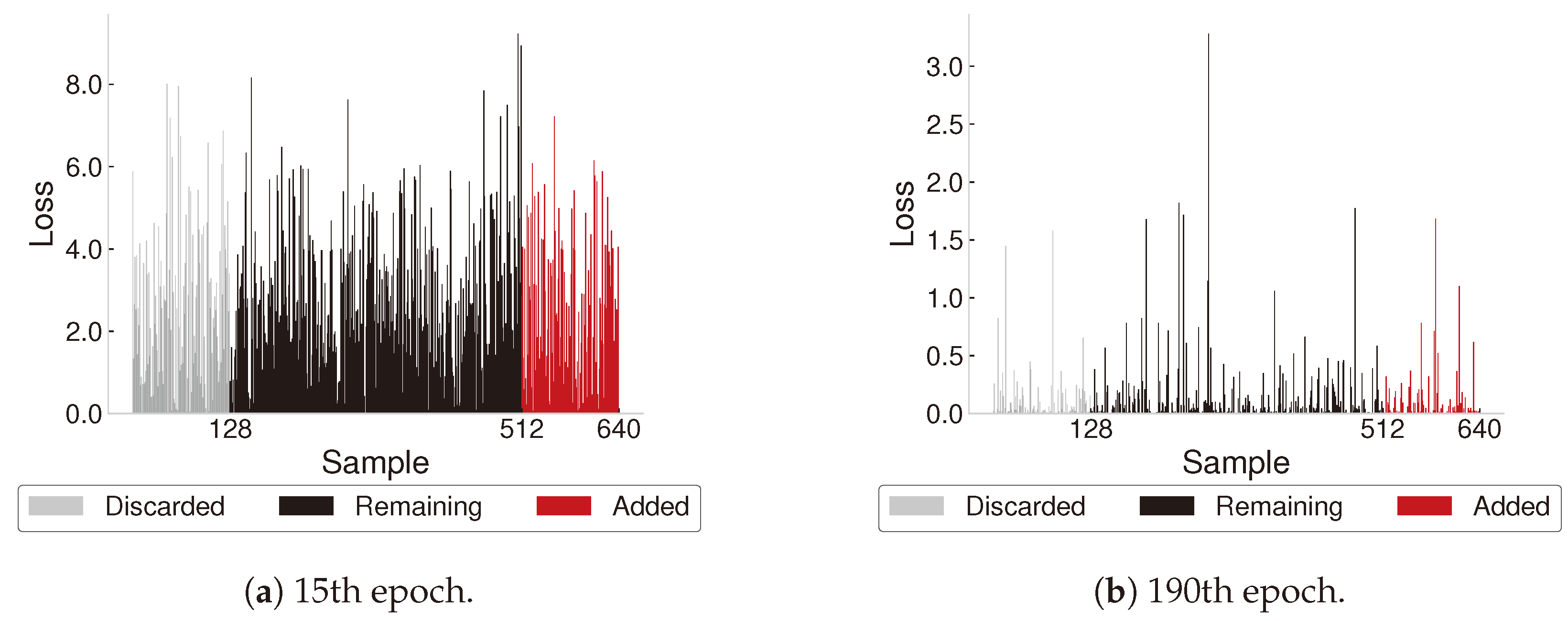
For a better understanding of ADONIS dynamics, it is important to inspect selected samples through the training process. This is further demonstrated by comparing selected samples during ResNet18 training on CIFAR-100 at 15th and 190th epochs. To begin with, the loss history is updated with every forward batch (Figure 2).
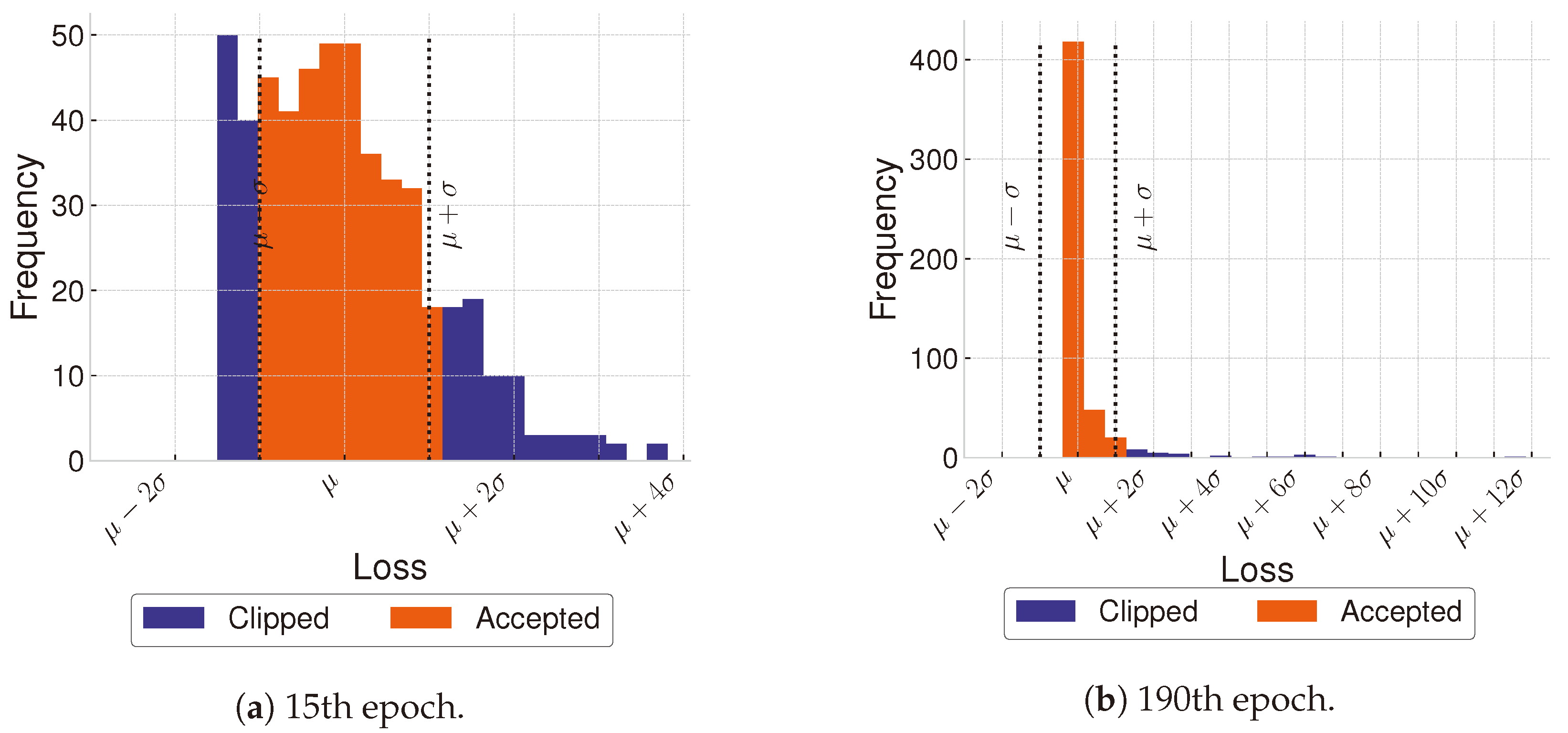
After that, the new state of the loss history is analyzed from the perspective of loss distribution and clipped due to a certain amount of standard distribution σ , as depicted in Figure 3.
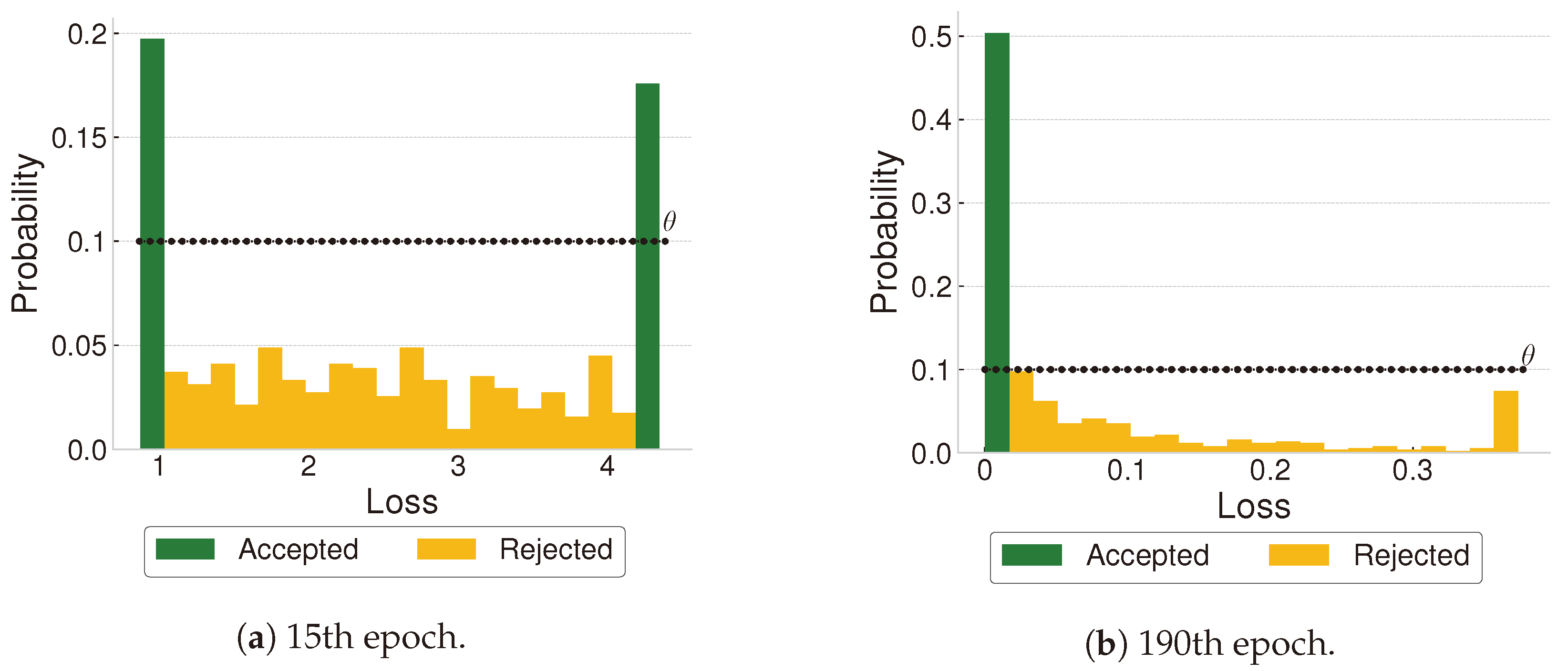
During the next step, a histogram is built from the current loss history and only bins that exceed the given probability threshold θ are accepted for the selection (Figure 4).
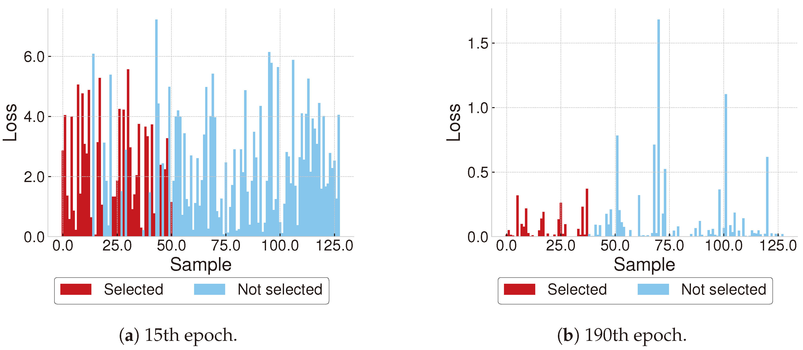
Finally, as illustrated in Figure 5, only samples that correspond to accepted bins are selected from a batch and are put into the training batch that is later used for backward step.
There are three distinct variances between the revised algorithm and its original counterpart. Initially, it is suggested to employ the novel ω parameter prior to transitioning to the training phase utilizing ADONIS (Algorithm 1). The second concept pertains to the computation of probabilities via the PMF in contrast to the initial proposition of utilizing the Cumulative Distribution Function (CDF). The proposed approach centers on prioritizing the most commonly occurring samples over the anomalous ones that incur the greatest losses because they might not only represent “hard” samples, but also wrongly annotated samples and outliers. The third approach involves the utilization of a deterministic probability threshold in the selection phase (3). This method stands in contrast to the probabilistic mode employed by the original SB. Given that ADONIS represents a notable advancement beyond the SB algorithm, it is of considerable import to elucidate the pertinent contrasts vis-à-vis extant implementations. There exist two open-source implementations: the first is the source code of the original paper as per reference [61], whereas the second is a constituent of the Composer library offering as per references [62,63]. The implementation of the Composer algorithm is not in line with the SB algorithm. Specifically, it utilizes a fixed number of chosen samples per batch, the selection is solely executed on the highest layer of a given batch, and it disregards loss history. Moreover, the computations for selection probabilities are not contingent on the actual loss values, while backpropagation is executed for each batch despite the fact that it may not be complete, resulting in costly additional backpropagation passes from a computational standpoint.

3.2. Intellectual Data Selection

A conceptual notion for expediting the period of model training involves minimizing the number of samples before training actually starts. The act of diminishing the number of samples present in the training dataset results in a reduction of the overall epoch time and not a decrease in the step time. Such a reduction in sample quantity can potentially lead to optimization processes achieving better computational efficiency. The rationale behind the presence of redundant information in datasets has been extensively explored and documented in scholarly literature [20,21,64]. The identification of a core set for a particular dataset presents various obstacles, such as clearly defined selection criteria, restricted time allocations for the selection process, and the requirement for proof of convergence [17].
The proposed approach for the filtration of training datasets involves the curation of a diverse set of samples from every class represented in a dataset. To assess diversity among samples, it becomes indispensable to establish a distance metric denoted as d ( · , · ) . Notably, the utilization of Euclidean distance in the process of image comparison has been shown to yield inaccurate outcomes [65] if it is applied straightforwardly to images. In other words, when the distance of two dissimilar images is measured with Euclidean metric between corresponding tensors they might be considered to be close. For a comprehensive list of distance metrics applicable to grayscale images, readers are advised to consult the work of [66]. Despite the widespread use of metrics such as Peak Signal-to-Noise Ratio (PSNR) or Structural Similarity Index (SSIM) for image similarity measurement, these metrics have been reported to be inadequate for accurately reflecting human assessments of the similarity between images [67]. This is why in this paper we cultivate the idea of first projecting images to the latent space and calculating the distance between them as the distance between images with the help of Euclidean distance as a metric.
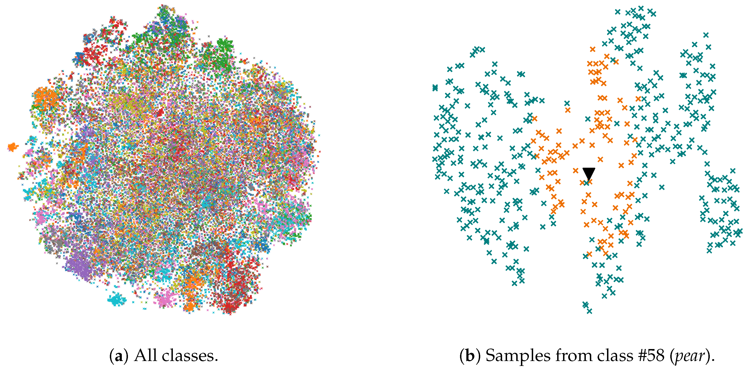
On the contrary, empirical evidence has shown that the image comparison that utilizes DL features derived from pre-trained models exhibits superior performance when viewed with regard to perceptual similarity, surpassing other metrics [67]. It is hereby recommended to commence the projection of dataset samples into a space of Z dimensions by utilizing the attributes of a pre-trained feature extractor, which will serve as the embedding function denoted as ϕ : D R Z . The present study has conducted experimentation on ResNet18 to investigate its efficacy. Upon projection into the latent space (Figure 6a), image similarity can be assessed by determining the Euclidean distance separating their respective embeddings as depicted in Equation (7).
d 2 ( x , y ) = k = 1 Z ( x ( k ) y ( k ) ) 2 x R Z , y R Z
Given the inherent structure of classification datasets, we posit the presence of duplicative information within each class, which may be removed without substantial impact on the ultimate precision of the analysis. As shown in [38], a conservative estimate suggests that a minimum of 10% of sample instances in both CIFAR-10 and ImageNet 2012 datasets possess such qualities. In one paper [38], it was proposed to utilize Hierarchical Clustering as a means to identify and group similar samples, ultimately enabling the removal of all but one representative from each grouping.
Accordingly, the identification of the prototype of the group is a prerequisite for the elimination of any individual cases. Considering that every sample is depicted in a latent space, there might exist diverse strategies to discover the aforementioned prototype. It is recommended to employ the K-Means clustering algorithm for the purpose of discerning class centroids. One primary motivation for employing K-Means clustering as opposed to the hierarchical approach stems from its potential applicability in the context of active learning. In particular, when novel samples emerge over time, it becomes crucial to assess their potential value for engaging in supplementary training processes [18].
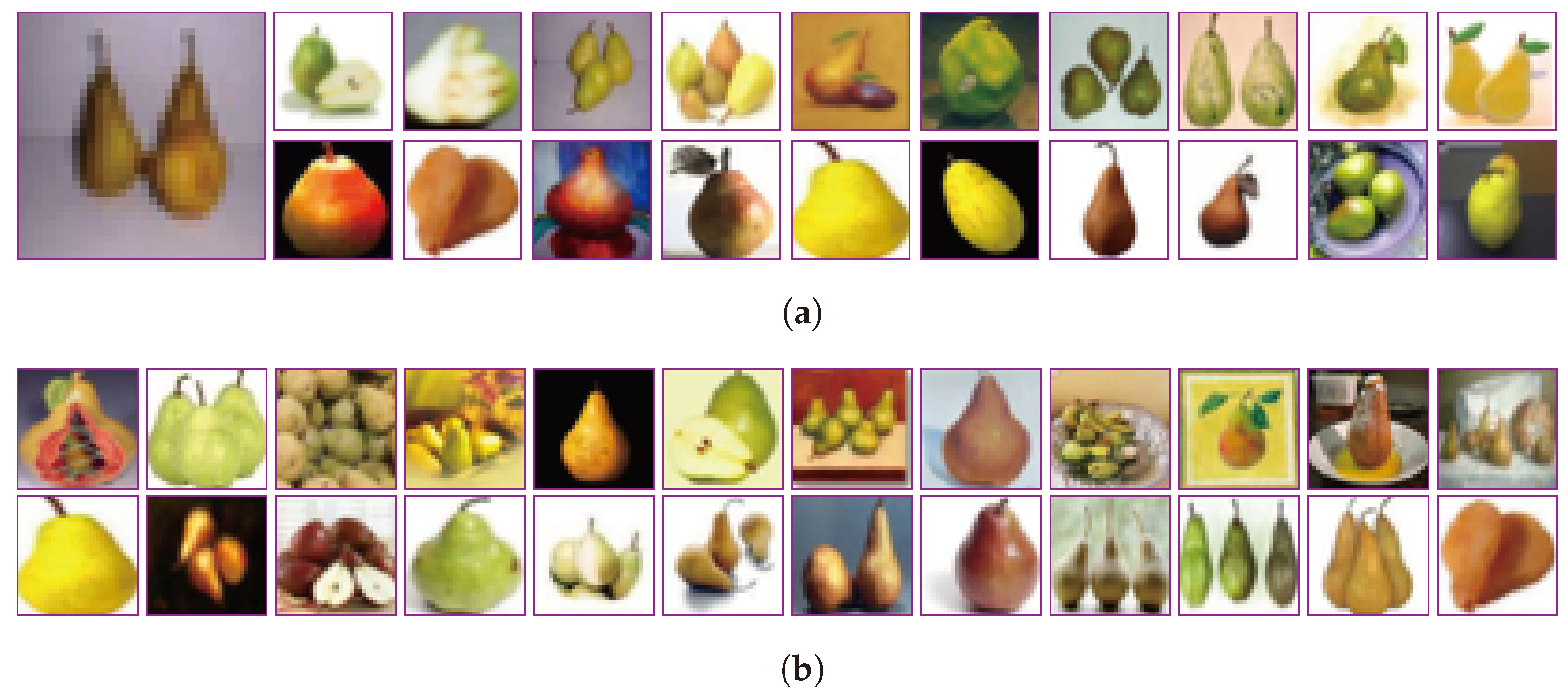
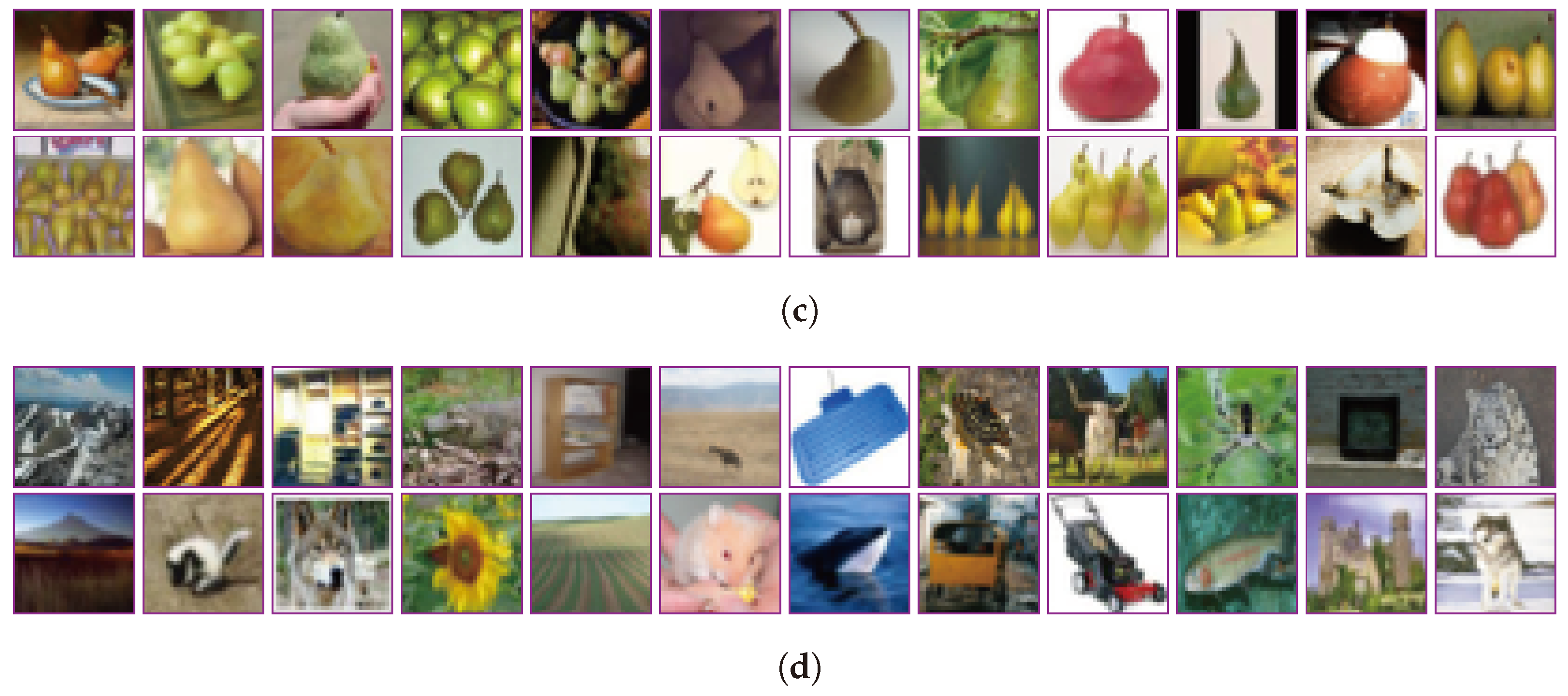
After centroids are detected for each class (Figure 6b), we identify samples that should be selected according to the selection ratio α ( 0 , 1 ] . In case α = 1 , training is run on the original dataset. Let all distributed representations of samples in the i-th class D i = { ξ 1 i , ξ 2 i , , ξ L i } , where L denotes number of samples in given class, be sorted in descending order according to the Euclidean distance to the centroid. Then, we select the first α L samples from D i . In addition, we insist on adding the last sample to this list, as it plays the role of the prototype for all samples removed from a class. As a result, we obtain a subset of the original dataset within a given selection ratio. The formal description of the proposed method is demonstrated in Algorithm 2 and Figure 6.
Algorithm 2 Intellectual Data Selection (IDS) algorithm
1:
M o d e : mode of selection {EASY, HARD}
2:
α : selection ratio
3:
ϕ : embedding function
4:
Q = { } : final dataset
5:
for each class D i in D do
6:
   L i = | D i | : number of samples in class
7:
   Ξ i = { inf } , | Ξ i | = L i : distributed representations of samples in D i
8:
  for each sample j in D i  do
9:
    ξ j i ϕ ( j ) : obtain distributed sample representation
10:
  end for
11:
   λ i K M e a n s ( Ξ i ) : find centroid of a cluster, i.e., class
12:
   Θ i = { inf } , | Ξ i | = L i : distances from samples to centroid λ i
13:
  for each sample j in D i  do
14:
    θ j i d ( j , λ i ) : calculate distance to centroid
15:
  end for
16:
   O i s o r t ( Θ , M o d e ) : sort samples w.r.t to their cluster centroid in ascending order if mode is EASY, descending otherwise
17:
   Q Q { O j i : j = 1 , 2 , , α L i } { O L i } : add selected samples to final dataset (including cluster prototype)
18:
end for
The key dissimilarity between IDS and SSP is performing clustering within individual classes as opposed to enumerating a predetermined number of clusters and conducting the operation on the entire training dataset. This method facilitates the prevention of imbalanced class selection scenarios and eliminates the requirement for the number of clusters as an algorithmic hyperparameter. The present proposal advocates the utilization of the Euclidean metric in lieu of the cosine similarity method as originally posited in the SSP paradigm.

4. Results

In the context of experimental evaluation, we employed four CV datasets: CIFAR-100 [68], CIFAR-10, ImageNet 2012 and MS COCO 2017 which are frequently utilized for the purpose of benchmarking the efficacy of training acceleration algorithms [20,22,51]. CIFAR-100 and CIFAR-10 datasets are partitioned such that there are 50 K images available for training purposes, while 10 K images are allotted specifically for testing. For CIFAR-100 there are 100 classes each containing 600 distinct 32 × 32 RGB examples, for CIFAR-10—10 classes with 6000 distinct 32 × 32 RGB examples. ImageNet 2012 consists of RGB images from 1000 different classes: 1.28 M for training and 50 K for validation. MS COCO 2017 is a dataset and consists of 118 K of training and 5K of validation RGB samples for object detection task, where the number of classes is equal to 80. When training on datasets the following common settings were used. For training on ImageNet 2012: mean = [0.485, 0.456, 0.406], std = [0.229, 0.224, 0.225] were used for samples normalization. For CIFAR-100: mean = [0.5070751592371323, 0.48654887331495095, 0.4409178433670343], std = [0.2673342858792401, 0.2564384629170883, 0.27615047132568404], for CIFAR-10: mean = [0.49139968, 0.48215827, 0.44653124], std = [0.24703233, 0.24348505, 0.26158768] for. The number of training epochs on ImageNet 2012 is 90, on CIFAR-100 and CIFAR-10—200, on MS COCO 2017—100.
With regards to the models that are currently under evaluation, our focus is 4 CV models: ResNet18 [69], ResNet50, MobileNet v2 [70], YOLO v5. The implementation of ResNet18, ResNet50 and MobileNet v2 and training pipelines for CIFAR-10 and CIFAR-100 datasets were taken from the official repository (https://github.com/weiaicunzai/pytorch-cifar100 (accessed on 15 June 2023)). Implementation of ResNet18, ResNet50 and MobileNet v2 for ImageNet 2012 was taken from torchvision library [71] v0.14.0. Training pipeline for YOLO v5 (yolov5m) training on MS COCO 2017 was used from ultralytics (https://github.com/ultralytics/yolov5 (accessed on 15 June 2023)) GitHub repository. For the needs of IDS, the pre-trained ResNet18 neural network implemented in the torchvision library is utilized as the embedding function. This involves the extraction of the 512-dimensional output from the penultimate layer. The weights for this model were obtained as a result of ResNet18 training on the ImageNet 2012 dataset [72] and have been made publicly available in the official repository.
The training protocol for ResNet18, ResNet50 and MobileNet v2 on CIFAR-100 and CIFAR-10 is as follows: the selected loss function is Cross Entropy, the optimizer is Stochastic Gradient Descent with a learning rate equal to 0.1, momentum is 0.9, and weight decay is 5 × 10 4 . The learning rate is dynamically reduced by a gamma equal to 0.2 during training at specified milestones: 60th, 120th, and 160th epochs. The data are loaded with 32 workers with a batch size equal to 128, randomly shuffled at each epoch. Each sample is processed with the following pipeline: random crop to size equal to 32 with padding equal to 4, then random horizontal flip, random rotation by angle, and sample normalization.
The training protocol for ResNet18 and ResNet50 on ImageNet 2012 is as follows: the selected loss function is Cross Entropy, the optimizer is Stochastic Gradient Descent with a learning rate equal to 0.1, momentum is 0.9, and weight decay is 1 × 10 4 . The learning rate is dynamically reduced by a gamma equal to 0.1 at each 30th epoch. The data are loaded with 32 workers with a batch size equal to 256, randomly shuffled at each epoch. Each sample is processed with the following pipeline: random crop to size equal to 224 with bilinear interpolation, then random horizontal flip and sample normalization.
The training protocol for MobileNet v2 on ImageNet 2012 is as follows: the selected loss function is Cross Entropy, the optimizer is Stochastic Gradient Descent with a learning rate equal to 0.045, momentum is 0.9, and weight decay is 4 × 10 5 . The learning rate is dynamically reduced by a gamma equal to 0.98 at each training epoch. The data are loaded with 32 workers with a batch size equal to 256, randomly shuffled at each epoch. Each sample is processed with the following pipeline: random crop to size equal to 224 with bilinear interpolation, then random horizontal flip and sample normalization.
The training protocol for YOLO v5 on MS COCO 2017 is as follows: the selected loss is the cumulative sum of bounding box regression, classification, and confidence losses, the optimizer is Stochastic Gradient Descent with a learning rate equal to 0.01, momentum is 0.937, and weight decay is 4 × 10 5 . The learning rate is dynamically reduced by a gamma equal to 0.98 at each training epoch. The data are loaded with eight workers with a batch size equal to 16, randomly shuffled at each epoch. All input samples during YOLO v5 training are resized to 640 pixels.
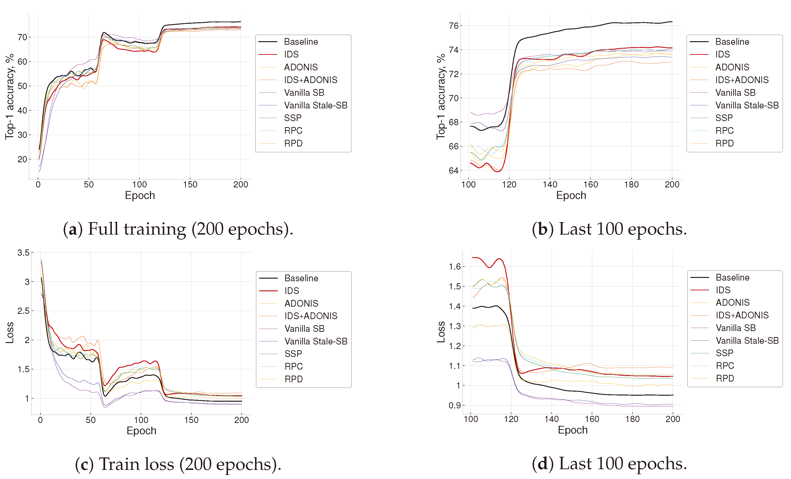
The overall dynamics of training is demonstrated as an example for ResNet18 training on CIFAR-100 in Figure 7. The present study employed various methodologies and their corresponding configurations to conduct a comparative analysis. The system under investigation was configured to include the SSP, Random Per Class (RPC), Random Per Dataset (RPD), ADONIS, and IDS. RPC means offline a reduction in the dataset by keeping only α samples from each class. RPD means an offline reduction in the dataset by keeping only α samples from the whole dataset regardless of the class it belongs to. The SB was initialized with the standard parameters of β = 2 , γ = 1024 , s t a l e n e s s = 2 .
All training experiments were performed on a single GPU device in mixed precision (full and half-precision floating point format) [73]. Certain hardware optimizations were enabled: pinning memory for data loaders (pin_memory = True) and benchmarking mode (cudnn.benchmark = True). For training evaluation experiments, the following hardware was used: CPU is Intel(R) Xeon(R) Gold 6151 CPU @ 3.00 GHz with 32 cores (frequency not fixed), OS: Ubuntu 20.04 LTS, kernel version: 5.4.0-136-generic; GPU is 1x NVIDIA Tesla V100 PCIe 16GB, driver version: 470.129.06, CUDA: 11.7; training framework: PyTorch 1.13.0, programming language: Python 3.9. K-Means algorithm implementation is taken from scikit-learn library v1.1.2. Additional libraries: imageio library v2.26.0, numpy library v1.21.5, opencv-python library v4.7.0.72, Pillow library v9.3.0, pycocotools library v2.0.6.
The present study showcases a comprehensive evaluation of the efficacy of training acceleration methods, as illustrated in Table A1 for ImageNet 2012, CIFAR-100, CIFAR-10, employing the aforementioned configurations. The quantification of the decrease in accuracy, commonly referred to as Accuracy drop, is determined in absolute percentage points for each method in relation to its corresponding baseline. The present study entails a comparative analysis of the efficiency of several algorithms, namely IDS, SSP, Random, and ADONIS, against the default baseline. Additionally, the performance of the Vanilla SB algorithm is assessed against its eponymous baselines. These findings are presented in Table 1. Boost is determined by taking the ratio of the duration of training with the standard baseline approach to the duration of training achieved when utilizing an acceleration algorithm during training of ResNet18.
The best results for training research models on CIFAR-10, CIFAR-100, ImageNet 2012 and MS COCO 2017 are shown in Table A1. Application of Adaptive Online Importance Sampling to ResNet50 training on ImageNet 2012 results in 2.37 times quicker convergence to 71.7% top-1 accuracy, which is within 5% from baseline. Total training time for the same number of epochs as in baseline is reduced by 1.82 times, with an accuracy drop of 2.45 p.p. The amount of time required to apply Intellectual Data Selection to ResNet50 training on ImageNet 2012 is decreased by 1.27 times with a corresponding decline in accuracy of 1.12 p.p. Applying both methods to ResNet50 training on ImageNet 2012 results in 2.31 speedup with an accuracy drop of 3.5 p.p.
It is imperative to acknowledge that approaches geared toward reducing datasets, such as SSP and IDS, necessitate preliminary preprocessing of the dataset. The processing time required by the SSP algorithm for handling CIFAR-100 amounts to 66.10 s, while it takes 28.82 s to process with IDS. For processing the CIFAR-10 dataset the SSP requires 31.90 s, while IDS will cope in 20.31 s. The SSP preprocessing for the ImageNet 2012 dataset will take 15,201.03 s, while IDS requires 10,019.81 s. Unlike SSP, IDS is able to process MS COCO 2017 in 1983.51 s. Evidently, the aforementioned duration is not encompassed within the documented period of training.
Furthermore, we present empirical evidence of enhanced model convergence through an evaluation of the rate at which a model trained using the acceleration method attains particular accuracy thresholds when compared to the ultimate baseline accuracy. As an illustration, ADONIS with a parameter value of η = 2 exhibits an acceleration ratio of 2.37 when subjected to a 5% reduction in accuracy. The results indicate that the utilization of the ADONIS algorithm during training of ResNet18 results in an achieved accuracy of 71.53%, which is found to deviate by no more than 5% from the final accuracy obtained via a default baseline. Furthermore, this approach yields a notable speedup of 2.37 compared to models that were trained without the incorporation of the ADONIS algorithm. The per-sample analysis is demonstrated in Figure 8.
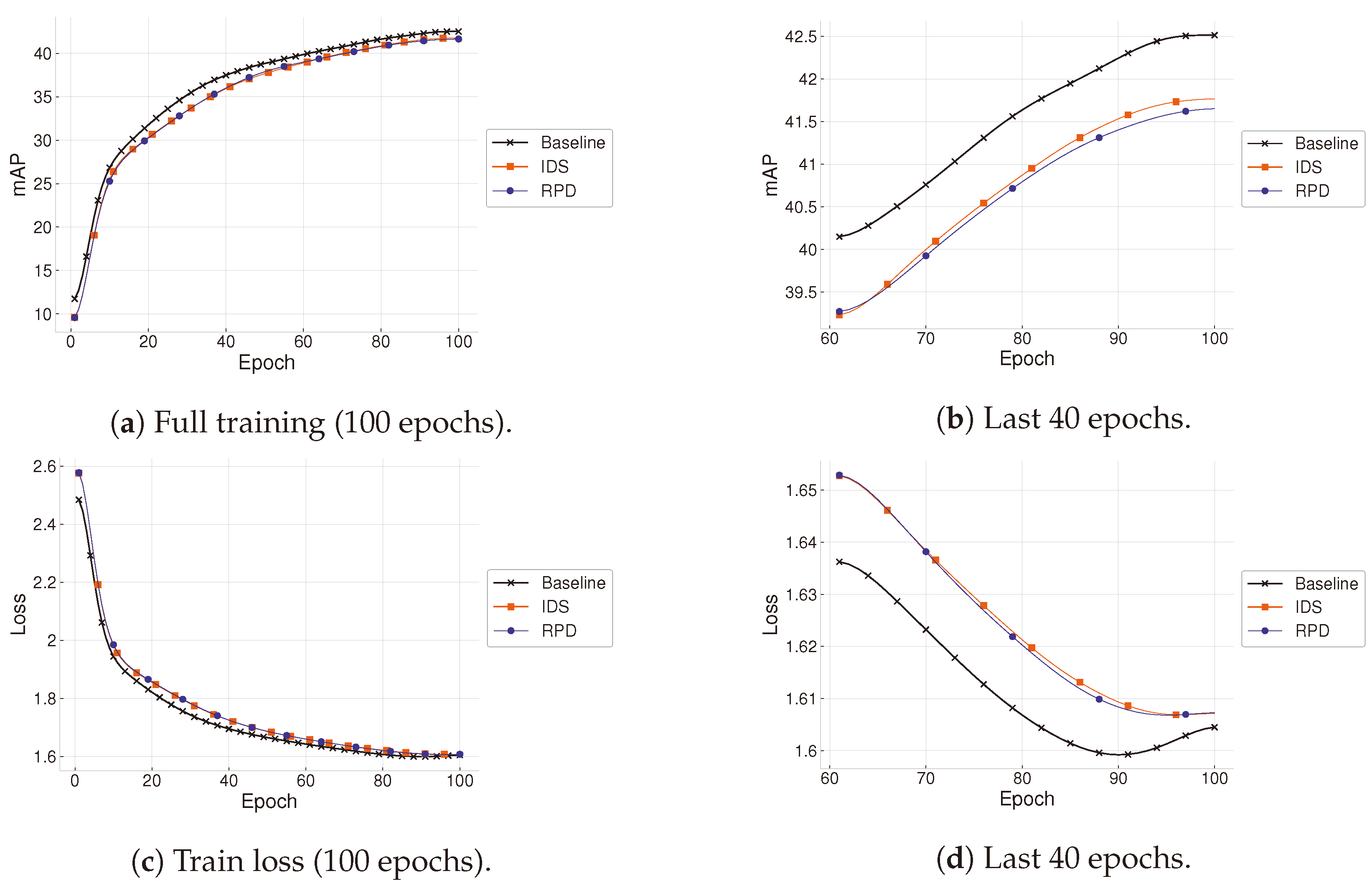
Beyond that, the results of measurements of IDS of object detection are presented in Table A1 and Figure 9. To apply IDS approach to the MS COCO 2017 dataset, where each sample could contain objects from different classes, we proposed to define one prototype in the entire dataset results show the possibility of reducing 20% of the MS COCO 2017 dataset with a mAP reduction of 0.76 p.p.

5. Discussion

5.1. Summary

In the present study, we introduce two novel methods: Adaptive Online Importance Sampling (ADONIS), and Intellectual Data Selection (IDS). The acceleration of training using the IDS approach is accomplished through the elimination of semantic redundancies within the training dataset. This results in a reduction in the number of training samples utilized for the study. Additionally, this approach involves the coordination of training procedures through the rigorous categorization of sample sets into distinct groups, namely those of easy and hard difficulty levels. ADONIS—a novel algorithmic approach—offers acceleration capabilities by means of minimizing the frequency of forward and backpropagation iterations observed during the training phase of DNN. The extent to which a given model is unable to appropriately identify certain data samples serves as the determining factor for the optimization measures imposed by ADONIS.
The proposed methods allow reducing the amount of data required to train a model of quality close to the baseline (full training), might be easily scaled to other CV and NLP tasks, and can be combined with other methods, for example during model fine-tuning [19].

5.2. Limitations and Outlook

One of the limitations of the current study pertains to the absence of extensive experimentation to establish the viability of the proposed methods on other CV tasks such as semantic segmentation. Addressing this limitation would pave the way for future research to leverage the proposed methods for scaling up image processing algorithms. It is of utmost significance to appropriately tailor the suggested methodologies to the sphere of NLP, given its emergence as one of the most arduous subdomains of DL. The application of distinct pre-trained models for feature extraction and various distance metrics for the training dataset pruning process represents a promising approach to enhance the performance of the IDS. Distance metric selection constitutes a pivotal area of investigation within our research endeavor.
There are several potential areas for improvement in ADONIS. One of the major concepts is to eliminate the extra step required to calculate selection probabilities and choose samples. By increasing the batch size in the selection process, this supplement might be lessened. The second strategy to enhance ADONIS involves computing sample probability using a weighted histogram. The overall idea is to allow a bigger impact on the most recent losses as they are obtained with a more up-to-date model. Third, it is possible to eliminate extra computations of losses that are duplicated for each sample during selection and backward passes. Reusing calculated loss might significantly increase ADONIS speed as additional forward passes and losses computations make up the majority of the selection process.
We define the following development horizons from the perspective of IDS improvement. The first direction is linked to the change from looking for one prototype per class to looking for several prototypes. This makes it possible to identify unused samples more precisely and prevent accuracy loss. Analyzing the capacity to alter the dataset more than once using a particular set of γ parameters is another topic of inquiry. We can decrease the forgetting component of the model, which can boost the resulting accuracy, by repeatedly swapping the dataset between “easy” and “hard” examples. Finding prototypes without using the clustering approach is one of the intriguing areas for the development of the IDS.
In conclusion, the presented methodologies exhibit significant promise in enhancing the efficiency of CNN training through the reduction of training data prior to and during the training phase while surpassing current solutions in this domain.

Author Contributions

Conceptualization, A.D.; Data curation, A.T. (Artyom Tugaryov) and A.T. (Aleksei Trutnev); Funding acquisition, S.P.; Investigation, A.D.; Methodology, A.D.; Project administration, S.P.; Software, A.T. (Artyom Tugaryov), A.T. (Aleksei Trutnev), M.K. and I.S.; Supervision, A.D. and S.P.; Validation, A.T. (Artyom Tugaryov), A.T. (Aleksei Trutnev), M.K. and I.S.; Visualization, A.T. (Artyom Tugaryov) and A.T. (Aleksei Trutnev); Writing—original draft, A.D.; Writing—review and editing, A.D. and S.P. All authors have read and agreed to the published version of the manuscript.

Funding

This research received no external funding.

Data Availability Statement

Data are available in a publicly accessible repository that does not issue DOIs. Publicly available datasets were analyzed in this study. This data can be found here: CIFAR-100, CIFAR-10: [https://www.cs.toronto.edu/~kriz/cifar.html (accessed on 15 June 2023)], ImageNet 2012: [https://www.image-net.org/ (accessed on 15 June 2023)], MS COCO 2017: [https://cocodataset.org/ (accessed on 15 June 2023)].

Conflicts of Interest

The authors declare no conflict of interest.

Appendix A. Detailed Results on CV Datasets

Extended results on evaluation of proposed methods on ImageNet 2012, CIFAR-100, CIFAR-10 and MS COCO 2017 are demonstrated in Table A1.
Table A1. Evaluation of training acceleration for selected computer vision models on ImageNet 2012, CIFAR-100, CIFAR-10 and MS COCO 2017. All results are grouped in sections, each section stands for a unique combination of a model and a dataset. Bold represents a result that is the best across given range of methods within a section.
DatasetModelMethodAcc. Drop (Full Train), p.p.Train Boost (Full Train), xBoost to 5 p.p. Drop, x
CIFAR-10ResNet18IDS ( γ = 180 )0.721.213.91
ADONIS ( η = 1 )0.761.284.0
ADONIS ( η = 2 )0.771.414.05
ADONIS ( η = 3 )0.551.464.35
IDS ( γ = 120 ) + ADONIS ( η = 1 )1.271.584.08
IDS ( γ = 120 ) + ADONIS ( η = 2 )1.051.754.87
IDS ( γ = 120 ) + ADONIS ( η = 3 )1.291.814.99
SSP0.651.243.97
RPC0.741.233.95
RPD0.531.233.93
CIFAR-10ResNet50IDS ( γ = 180 )0.451.224.01
ADONIS ( η = 1 )0.971.353.77
ADONIS ( η = 2 )0.991.524.07
ADONIS ( η = 3 )0.981.694.49
IDS ( γ = 120 ) + ADONIS ( η = 1 )1.621.592.62
IDS ( γ = 120 ) + ADONIS ( η = 2 )1.691.762.79
IDS ( γ = 120 ) + ADONIS ( η = 3 )1.651.933.05
SSP0.781.183.79
RPC0.381.183.87
RPD0.581.193.95
CIFAR-10MobileNet v2IDS ( γ = 180 )−0.241.271.72
ADONIS ( η = 1 )0.441.391.86
ADONIS ( η = 2 )0.191.592.08
ADONIS ( η = 3 )0.41.682.18
IDS ( γ = 120 ) + ADONIS ( η = 1 )1.041.752.31
IDS ( γ = 120 ) + ADONIS ( η = 2 )1.171.962.56
IDS ( γ = 120 ) + ADONIS ( η = 3 )0.962.042.66
SSP0.551.281.73
RPC0.231.191.62
RPD0.291.131.53
CIFAR-100ResNet18IDS ( γ = 120 )2.121.151.9
ADONIS ( η = 1 )2.761.161.83
ADONIS ( η = 2 )2.51.231.97
ADONIS ( η = 3 )2.661.272.03
IDS ( γ = 120 ) + ADONIS ( η = 1 )3.551.582.5
IDS ( γ = 120 ) + ADONIS ( η = 2 )3.261.712.72
IDS ( γ = 120 ) + ADONIS ( η = 3 )3.261.752.76
Vanilla SB2.430.922.84
Vanilla Stale-SB2.811.11.8
SSP2.321.143.63
RPC2.491.292.12
RPD2.431.161.91
CIFAR-100ResNet50IDS ( γ = 120 )1.881.221.85
ADONIS ( η = 1 )2.21.321.96
ADONIS ( η = 2 )2.361.562.28
ADONIS ( η = 3 )2.191.632.37
IDS ( γ = 120 ) + ADONIS ( η = 1 )4.241.612.21
IDS ( γ = 120 ) + ADONIS ( η = 2 )4.651.892.1
IDS ( γ = 120 ) + ADONIS ( η = 3 )4.921.92.08
SSP2.741.171.76
RPC2.771.181.79
RPD2.131.181.78
CIFAR-100MobileNet v2IDS ( γ = 120 )1.821.31.73
ADONIS ( η = 1 )1.91.541.94
ADONIS ( η = 2 )1.871.72.14
ADONIS ( η = 3 )1.371.772.23
IDS ( γ = 120 ) + ADONIS ( η = 1 )2.771.781.96
IDS ( γ = 120 ) + ADONIS ( η = 2 )3.411.992.05
IDS ( γ = 120 ) + ADONIS ( η = 3 )3.72.082.06
SSP0.961.271.69
RPC1.591.211.6
RPD1.631.211.61
ImageNet 2012ResNet18IDS ( γ = 14 )1.21.221.72
ADONIS ( η = 1 )2.551.11.53
ADONIS ( η = 2 )2.391.111.54
ADONIS ( η = 3 )2.511.111.54
IDS ( γ = 14 ) + ADONIS ( η = 1 )3.641.632.23
IDS ( γ = 14 ) + ADONIS ( η = 2 )3.841.662.25
IDS ( γ = 14 ) + ADONIS ( η = 3 )3.741.742.35
SSP4.411.221.52
RPC4.641.221.51
RPD4.521.221.52
ImageNet 2012ResNet50IDS ( γ = 14 )1.121.271.81
ADONIS ( η = 1 )2.181.482.02
ADONIS ( η = 2 )2.41.712.27
ADONIS ( η = 3 )2.451.822.37
IDS ( γ = 14 ) + ADONIS ( η = 1 )3.481.772.37
IDS ( γ = 14 ) + ADONIS ( η = 2 )3.432.172.88
IDS ( γ = 14 ) + ADONIS ( η = 3 )3.52.313.05
SSP4.031.231.67
RPC4.221.251.62
RPD4.171.281.66
ImageNet 2012MobileNet v2IDS ( γ = 14 )0.611.252.61
ADONIS ( η = 1 )2.251.62.46
ADONIS ( η = 2 )1.741.722.66
ADONIS ( η = 3 )1.911.872.99
IDS ( γ = 14 ) + ADONIS ( η = 1 )3.361.952.62
IDS ( γ = 14 ) + ADONIS ( η = 2 )3.362.192.82
IDS ( γ = 14 ) + ADONIS ( η = 3 )3.382.32.95
SSP0.331.242.85
RPC0.731.252.45
RPD0.831.252.69
MS COCO 2017YOLO v5IDS ( γ = 60 )0.761.192.41
RPD0.861.232.46

Appendix B. Sensitivity Analysis of Hyperparameters Selection in ADONIS

Each hyperparameter of ADONIS algorithm was analyzed in terms of its impact on resulting accuracy of a trained model and training acceleration. Key results are demonstrated in Figure A1.
The measurement methodology is the following: ResNet18 model was trained on CIFAR-100 dataset with ADONIS method. Each time different ADONIS configurations were used and weights were re-initialized. Each experiment used default training settings enumerated in Table A2 with only one parameter changed—the one that was under close investigation. The default IDS γ parameter depends on the evaluated dataset. We used γ = 180 for CIFAR-10, for CIFAR-100—120, for ImageNet 2012—14 and for MS COCO 2017—60.
Table A2. Default settings of training acceleration algorithms.
MethodSettings
SSP α = 0.8
RPC α = 0.8
RPD α = 0.8
IDS α = 0.8 , ϕ = r e s n e t 18
ADONIS l = 512 , k = s q u a r e , σ = 1 , η = 1 , θ = 0.12
First, we consider θ as it controls the number of candidate samples by defining the minimum probability. The best acceleration of 1.79x is achieved with θ = 0.7 but results in a huge accuracy drop of 23.64 p.p. Optimal trade-off between acceleration and accuracy drop is achieved with θ = 0.1 : 1.36x boost and accuracy drop of 1.73 p.p. The acceptable range of the parameter is from 0.1 to 0.7 . When θ < 0.1 almost all samples are selected for backpropagation operation, and, therefore, there is no boost in this case. At the same time, when θ > 0.7 too few samples are selected, and the accuracy drop is dramatically huge.
Second, σ hyperparameter is analyzed. It is responsible for mitigating random outliers in losses. The maximum boost of 1.38x is achieved with σ = 0.5 also resulting in an accuracy drop 2.07 p.p. Changing the parameter’s value to σ = 1 results in 1.35x boost and an accuracy drop of 1.73 p.p. ADONIS is not sensitive to large σ values as the number of samples considered outliers is close to zero with no influence on final accuracy. It is curious that for σ = 2 the probabilities are distributed so that they do not exceed a given threshold, and this forces us to choose a special threshold ( θ = 0.1 ) for this value. This suggests that it is necessary to select the threshold for each model and dataset separately.
Third, k denotes a rule for the computation of the number of bins in the histogram. The best acceleration of 1.38x is achieved with k = s q r t and results in the accuracy drop of 2.02 p.p. At the same time, we suggest configuring k = S t u r g e s because accuracy drop for the hyperparameter value is 1.73 p.p, however boost is significant 1.35x. ADONIS is not sensitive to any of the selected rules: Sturges, Square Root, Rice.
Fourth, we inspect the influence of selected history length, defined as hyperparameter l. Maximum acceleration is achieved with l = 512 : 1.36x with an accuracy drop of 1.96 p.p. Almost the same acceleration (1.35x) can be achieved with a much smaller accuracy drop (1.57 p.p) by configuring l = 256 . We recommend specifying l as a number divisible by batch size.
Fifth, we analyze the influence of the hyperparameter α that is responsible for controlling the amount of selected samples from the candidate list. The most significant acceleration of 1.59x is achieved with the value of 0.1 resulting in an accuracy drop of 3.02 p.p. Optimal configuration is α = 0.3 as accuracy drop is smaller—1.73 p.p while boost is significant—1.35x. Figure A1e demonstrates that low values of this hyperparameter result in only a few samples being selected and, as a result, a dramatic accuracy drop. Specifying α > 0.7 results in a larger number of samples to be selected, eliminating any benefits from ADONIS.
Figure A1. Sensitivity analysis of ADONIS parameters.
Mathematics 11 03120 g0a1
Finally, parameter η which decreases the number of additional forward steps, delivers maximum acceleration of 1.53x with an accuracy drop 1.53 p.p for η = 3 . Due to Figure A1f this parameter allows for a considerable boost without compromising accuracy drop.
To sum up, ADONIS is sensitive to σ , η , θ and α and they are required to be tuned for a particular model and dataset. At the same time, other parameters such as k and l could be frozen at recommended values: k = S t u r g e s and l = 512 correspondingly.

Appendix C. Sensitivity Analysis of Hyperparameters Selection in IDS

Each hyperparameter of IDS algorithm was analyzed in terms of its impact on resulting accuracy of a trained model and training acceleration. Key results are demonstrated in Figure A2.
The measurement methodology is the following: ResNet18 model was trained on CIFAR-100 dataset with IDS method. Each time different IDS configurations were used and weights were re-initialized. Each experiment used default training settings enumerated in Table A2 with only one parameter changed—the one that was under close investigation.
The most crucial hyperparameter of IDS is selection ratio ( α ) as it provides an opportunity to decrease the number of samples used in the training process. The lower α is the bigger boost and corresponding accuracy drop are. The maximum acceleration of 1.36x is achieved with α = 0.5 but also results in a considerable accuracy drop of 6.29 p.p. When the ratio of selected samples is increased to α = 0.8 accuracy drop results in 2.19 p.p. with a boost of 1.13x. Specifying α < 0.5 is meaningless because it means removing more than half of a dataset with a quite expected significant accuracy drop as a consequence. On the other hand, α > 0.9 will not provide any perceptible boost.
Second, we analyzed γ parameter influence on training performance as it allows us to switch from samples close to the class prototype to samples that are more remote. Configuring γ > 180 does not allow the model to learn much about newly introduced samples which is reflected in an accuracy drop up to 2.7 p.p. At the same time, an earlier switch to the most remote samples ( γ = 160 ) allows for achieve acceptable accuracy drop of 1.88 p.p. with a boost of 1.21x.
Figure A2. Sensitivity analysis of IDS parameters.
Mathematics 11 03120 g0a2
Third, feature extractor ϕ is considered an important component that deserves analysis on its impact on training dynamics and final accuracy rates. The reason is that sample selection within IDS is performed based on the cluster analysis of training data represented in the latent space. As for feature extractors, several model architectures were selected. First, is the usage of ResNet18 model [74] with pre-trained weights (https://github.com/pytorch/vision/blob/main/torchvision/models/resnet.py (accessed on 15 June 2023)). Second, we used SwAV [75] model with pre-trained weights (https://github.com/facebookresearch/swav (accessed on 15 June 2023)) and ResNet50 as the backbone. SwAV is known to be one of the state-of-the-art models that learns visual features via self-supervised training on ImageNet 2012. Third, a recently proposed DINOv2 model [76] was inspected. The latter achieves remarkable results on various CV tasks, although being trained in a self-supervised manner. DINOv2 weights were taken from publicly available storage (https://github.com/facebookresearch/dinov2 (accessed on 15 June 2023)). Therefore, it might be considered a robust and qualitative feature extractor. Alongside with pre-trained models, we also experimented with ResNet18 model snapshots from 5th, 10th, 15th epochs. A summary of used feature extractors is included in Table A3. Evaluation results are demonstrated in Figure A2c. Reducing a dataset by performing clustering of samples based on latent representation produced by ResNet18 (15th epoch) negligibly outperforms other extractors. This is explained by large γ values, which anyway allow a model to focus on training the majority of samples, while still being able to extract proper features from training data and achieve appropriate validation accuracy.
Table A3. Feature extractors under evaluation.
ModelLatent Space
ResNet18512
ResNet18 (5)512
ResNet18 (10)512
ResNet18 (15)512
SwAV2048
DINOv2384

References

  1. Shen, D.; Wu, G.; Suk, H.I. Deep learning in medical image analysis. Annu. Rev. Biomed. Eng. 2017, 19, 221. [Google Scholar] [CrossRef] [Green Version]
  2. Tuncer, T.; Ertam, F.; Dogan, S.; Aydemir, E.; Pławiak, P. Ensemble residual network-based gender and activity recognition method with signals. J. Supercomput. 2020, 76, 2119–2138. [Google Scholar] [CrossRef]
  3. Vaswani, A.; Shazeer, N.; Parmar, N.; Uszkoreit, J.; Jones, L.; Gomez, A.N.; Kaiser, Ł.; Polosukhin, I. Attention is all you need. Adv. Neural Inf. Process. Syst. 2017, 30, 5998–6008. [Google Scholar]
  4. Andrychowicz, O.M.; Baker, B.; Chociej, M.; Jozefowicz, R.; McGrew, B.; Pachocki, J.; Petron, A.; Plappert, M.; Powell, G.; Ray, A.; et al. Learning dexterous in-hand manipulation. Int. J. Robot. Res. 2020, 39, 3–20. [Google Scholar] [CrossRef] [Green Version]
  5. Zhu, H.; Yuen, K.V.; Mihaylova, L.; Leung, H. Overview of environment perception for intelligent vehicles. IEEE Trans. Intell. Transp. Syst. 2017, 18, 2584–2601. [Google Scholar] [CrossRef] [Green Version]
  6. Janai, J.; Güney, F.; Behl, A.; Geiger, A. Computer vision for autonomous vehicles: Problems, datasets and state of the art. Found. Trends® Comput. Graph. Vis. 2020, 12, 1–308. [Google Scholar] [CrossRef]
  7. Silver, D.; Hubert, T.; Schrittwieser, J.; Antonoglou, I.; Lai, M.; Guez, A.; Lanctot, M.; Sifre, L.; Kumaran, D.; Graepel, T.; et al. A general reinforcement learning algorithm that masters chess, shogi, and Go through self-play. Science 2018, 362, 1140–1144. [Google Scholar] [CrossRef] [PubMed] [Green Version]
  8. Rydning, D.R.J.G.J.; Reinsel, J.; Gantz, J. The digitization of the world from edge to core. Fram. Int. Data Corp. 2018, 16, 1–28. [Google Scholar]
  9. Russakovsky, O.; Deng, J.; Su, H.; Krause, J.; Satheesh, S.; Ma, S.; Huang, Z.; Karpathy, A.; Khosla, A.; Bernstein, M.; et al. Imagenet large scale visual recognition challenge. Int. J. Comput. Vis. 2015, 115, 211–252. [Google Scholar] [CrossRef] [Green Version]
  10. Sun, C.; Shrivastava, A.; Singh, S.; Gupta, A. Revisiting unreasonable effectiveness of data in deep learning era. In Proceedings of the IEEE International Conference on Computer Vision, Venice, Italy, 22–29 October 2017; pp. 843–852. [Google Scholar]
  11. Zhai, X.; Kolesnikov, A.; Houlsby, N.; Beyer, L. Scaling vision transformers. In Proceedings of the IEEE/CVF Conference on Computer Vision and Pattern Recognition, New Orleans, LA, USA, 18–24 June 2022; pp. 12104–12113. [Google Scholar]
  12. Krizhevsky, A.; Sutskever, I.; Hinton, G.E. Imagenet classification with deep convolutional neural networks. Commun. ACM 2017, 60, 84–90. [Google Scholar] [CrossRef] [Green Version]
  13. Brown, T.; Mann, B.; Ryder, N.; Subbiah, M.; Kaplan, J.D.; Dhariwal, P.; Neelakantan, A.; Shyam, P.; Sastry, G.; Askell, A.; et al. Language models are few-shot learners. Adv. Neural Inf. Process. Syst. 2020, 33, 1877–1901. [Google Scholar]
  14. OpenAI. GPT-4 Technical Report. arXiv 2023, arXiv:2303.08774. [Google Scholar]
  15. Knight, W. A New Chip Cluster Will Make Massive AI Models Possible. 2023. Available online: https://www.wired.com/story/cerebras-chip-cluster-neural-networks-ai/ (accessed on 15 June 2023).
  16. Strubell, E.; Ganesh, A.; McCallum, A. Energy and policy considerations for deep learning in NLP. arXiv 2019, arXiv:1906.02243. [Google Scholar]
  17. Mirzasoleiman, B.; Bilmes, J.; Leskovec, J. Coresets for data-efficient training of machine learning models. In Proceedings of the International Conference on Machine Learning, PMLR, Virtual Event, 13–18 July 2020; pp. 6950–6960. [Google Scholar]
  18. Sener, O.; Savarese, S. Active learning for convolutional neural networks: A core-set approach. arXiv 2017, arXiv:1708.00489. [Google Scholar]
  19. Hu, E.J.; Shen, Y.; Wallis, P.; Allen-Zhu, Z.; Li, Y.; Wang, S.; Wang, L.; Chen, W. Lora: Low-rank adaptation of large language models. arXiv 2021, arXiv:2106.09685. [Google Scholar]
  20. Jiang, A.H.; Wong, D.L.K.; Zhou, G.; Andersen, D.G.; Dean, J.; Ganger, G.R.; Joshi, G.; Kaminksy, M.; Kozuch, M.; Lipton, Z.C.; et al. Accelerating deep learning by focusing on the biggest losers. arXiv 2019, arXiv:1910.00762. [Google Scholar]
  21. Sorscher, B.; Geirhos, R.; Shekhar, S.; Ganguli, S.; Morcos, A.S. Beyond neural scaling laws: Beating power law scaling via data pruning. arXiv 2022, arXiv:2206.14486. [Google Scholar]
  22. Cui, J.; Wang, R.; Si, S.; Hsieh, C.J. DC-BENCH: Dataset Condensation Benchmark. arXiv 2022, arXiv:2207.09639. [Google Scholar]
  23. Lei, S.; Tao, D. A Comprehensive Survey to Dataset Distillation. arXiv 2023, arXiv:2301.05603. [Google Scholar]
  24. Mayer, R.; Jacobsen, H.A. Scalable deep learning on distributed infrastructures: Challenges, techniques, and tools. ACM Comput. Surv. (CSUR) 2020, 53, 1–37. [Google Scholar] [CrossRef] [Green Version]
  25. Verbraeken, J.; Wolting, M.; Katzy, J.; Kloppenburg, J.; Verbelen, T.; Rellermeyer, J.S. A survey on distributed machine learning. Acm Comput. Surv. (CSUR) 2020, 53, 1–33. [Google Scholar]
  26. Wang, H.; Qu, Z.; Zhou, Q.; Zhang, H.; Luo, B.; Xu, W.; Guo, S.; Li, R. A comprehensive survey on training acceleration for large machine learning models in IoT. IEEE Internet Things J. 2021, 9, 939–963. [Google Scholar]
  27. Gupta, S.; Agrawal, A.; Gopalakrishnan, K.; Narayanan, P. Deep learning with limited numerical precision. In Proceedings of the International Conference on Machine Learning, PMLR, Lille, France, 7–9 July 2015; pp. 1737–1746. [Google Scholar]
  28. Zhou, S.; Wu, Y.; Ni, Z.; Zhou, X.; Wen, H.; Zou, Y. Dorefa-net: Training low bitwidth convolutional neural networks with low bitwidth gradients. arXiv 2016, arXiv:1606.06160. [Google Scholar]
  29. Seide, F.; Fu, H.; Droppo, J.; Li, G.; Yu, D. 1-bit stochastic gradient descent and its application to data-parallel distributed training of speech dnns. In Proceedings of the Fifteenth Annual Conference of the International Speech Communication Association, Singapore, 14–18 September 2014. [Google Scholar]
  30. Wen, W.; Xu, C.; Yan, F.; Wu, C.; Wang, Y.; Chen, Y.; Li, H. Terngrad: Ternary gradients to reduce communication in distributed deep learning. Adv. Neural Inf. Process. Syst. 2017, 30, 1509–1519. [Google Scholar]
  31. Liang, T.; Glossner, J.; Wang, L.; Shi, S.; Zhang, X. Pruning and quantization for deep neural network acceleration: A survey. Neurocomputing 2021, 461, 370–403. [Google Scholar]
  32. Lym, S.; Choukse, E.; Zangeneh, S.; Wen, W.; Sanghavi, S.; Erez, M. Prunetrain: Fast neural network training by dynamic sparse model reconfiguration. In Proceedings of the International Conference for High Performance Computing, Networking, Storage and Analysis, Denver, CO, USA, 17–22 November 2019; pp. 1–13. [Google Scholar]
  33. Google. Edge TPU. 2023. Available online: https://cloud.google.com/edge-tpu/ (accessed on 26 January 2023).
  34. Corporation, N. GeForce RTX 30 Series. 2023. Available online: https://www.nvidia.com/en-gb/geforce/graphics-cards/30-series/ (accessed on 15 June 2023).
  35. Huawei Technologies Co., Ltd. Ascend 910 Series. 2023. Available online: https://e.huawei.com/ae/products/cloud-computing-dc/atlas/ascend-910 (accessed on 15 June 2023).
  36. Vepakomma, P.; Gupta, O.; Swedish, T.; Raskar, R. Split learning for health: Distributed deep learning without sharing raw patient data. arXiv 2018, arXiv:1812.00564. [Google Scholar]
  37. Kang, Y.; Hauswald, J.; Gao, C.; Rovinski, A.; Mudge, T.; Mars, J.; Tang, L. Neurosurgeon: Collaborative intelligence between the cloud and mobile edge. ACM SIGARCH Comput. Archit. News 2017, 45, 615–629. [Google Scholar] [CrossRef] [Green Version]
  38. Birodkar, V.; Mobahi, H.; Bengio, S. Semantic Redundancies in Image-Classification Datasets: The 10% You Do not Need. arXiv 2019, arXiv:1901.11409. [Google Scholar]
  39. Toneva, M.; Sordoni, A.; Combes, R.T.d.; Trischler, A.; Bengio, Y.; Gordon, G.J. An empirical study of example forgetting during deep neural network learning. arXiv 2018, arXiv:1812.05159. [Google Scholar]
  40. Cazenavette, G.; Wang, T.; Torralba, A.; Efros, A.A.; Zhu, J.Y. Dataset distillation by matching training trajectories. In Proceedings of the IEEE/CVF Conference on Computer Vision and Pattern Recognition, New Orleans, LA, USA, 18–24 June 2022; pp. 4750–4759. [Google Scholar]
  41. Wang, T.; Zhu, J.Y.; Torralba, A.; Efros, A.A. Dataset distillation. arXiv 2018, arXiv:1811.10959. [Google Scholar]
  42. Coleman, C.; Yeh, C.; Mussmann, S.; Mirzasoleiman, B.; Bailis, P.; Liang, P.; Leskovec, J.; Zaharia, M. Selection via proxy: Efficient data selection for deep learning. arXiv 2019, arXiv:1906.11829. [Google Scholar]
  43. Shim, J.h.; Kong, K.; Kang, S.J. Core-set sampling for efficient neural architecture search. arXiv 2021, arXiv:2107.06869. [Google Scholar]
  44. Johnson, T.B.; Guestrin, C. Training deep models faster with robust, approximate importance sampling. Adv. Neural Inf. Process. Syst. 2018, 31, 7265–7275. [Google Scholar]
  45. Katharopoulos, A.; Fleuret, F. Biased importance sampling for deep neural network training. arXiv 2017, arXiv:1706.00043. [Google Scholar]
  46. Katharopoulos, A.; Fleuret, F. Not all samples are created equal: Deep learning with importance sampling. In Proceedings of the International Conference on Machine Learning, PMLR, Stockholm, Sweden, 10–15 July 2018; pp. 2525–2534. [Google Scholar]
  47. Zhang, Z.; Chen, Y.; Saligrama, V. Efficient training of very deep neural networks for supervised hashing. In Proceedings of the IEEE Conference on Computer Vision and Pattern Recognition, Las Vegas, NV, USA, 26 June–1 July 2016; pp. 1487–1495. [Google Scholar]
  48. Dogra, A.S.; Redman, W. Optimizing neural networks via Koopman operator theory. Adv. Neural Inf. Process. Syst. 2020, 33, 2087–2097. [Google Scholar]
  49. Lagani, G.; Falchi, F.; Gennaro, C.; Amato, G. Hebbian semi-supervised learning in a sample efficiency setting. Neural Netw. 2021, 143, 719–731. [Google Scholar] [CrossRef]
  50. Amato, G.; Carrara, F.; Falchi, F.; Gennaro, C.; Lagani, G. Hebbian learning meets deep convolutional neural networks. In Proceedings of the Image Analysis and Processing–ICIAP 2019: 20th International Conference, Trento, Italy, 9–13 September 2019; Proceedings, Part I 20. Springer: Berlin/Heidelberg, Germany, 2019; pp. 324–334. [Google Scholar]
  51. Krithivasan, S.; Sen, S.; Venkataramani, S.; Raghunathan, A. Accelerating DNN Training Through Selective Localized Learning. Front. Neurosci. 2022, 15, 759807. [Google Scholar] [CrossRef]
  52. Talloen, J.; Dambre, J.; Vandesompele, A. PyTorch-Hebbian: Facilitating local learning in a deep learning framework. arXiv 2021, arXiv:2102.00428. [Google Scholar]
  53. Miconi, T. Hebbian learning with gradients: Hebbian convolutional neural networks with modern deep learning frameworks. arXiv 2021, arXiv:2107.01729. [Google Scholar]
  54. Cekic, M.; Bakiskan, C.; Madhow, U. Towards robust, interpretable neural networks via Hebbian/anti-Hebbian learning: A software framework for training with feature-based costs. Softw. Impacts 2022, 13, 100347. [Google Scholar] [CrossRef]
  55. Moraitis, T.; Toichkin, D.; Journé, A.; Chua, Y.; Guo, Q. SoftHebb: Bayesian inference in unsupervised Hebbian soft winner-take-all networks. Neuromorphic Comput. Eng. 2022, 2, 044017. [Google Scholar] [CrossRef]
  56. Tang, J.; Yuan, F.; Shen, X.; Wang, Z.; Rao, M.; He, Y.; Sun, Y.; Li, X.; Zhang, W.; Li, Y.; et al. Bridging biological and artificial neural networks with emerging neuromorphic devices: Fundamentals, progress, and challenges. Adv. Mater. 2019, 31, 1902761. [Google Scholar] [CrossRef]
  57. Lagani, G.; Gennaro, C.; Fassold, H.; Amato, G. FastHebb: Scaling Hebbian Training of Deep Neural Networks to ImageNet Level. In Proceedings of the Similarity Search and Applications: 15th International Conference, SISAP 2022, Bologna, Italy, 5–7 October 2022; Springer: Berlin/Heidelberg, Germany, 2022; pp. 251–264. [Google Scholar]
  58. Journé, A.; Rodriguez, H.G.; Guo, Q.; Moraitis, T. Hebbian deep learning without feedback. arXiv 2022, arXiv:2209.11883. [Google Scholar]
  59. Lagani, G.; Falchi, F.; Gennaro, C.; Amato, G. Comparing the performance of Hebbian against backpropagation learning using convolutional neural networks. Neural Comput. Appl. 2022, 34, 6503–6519. [Google Scholar] [CrossRef]
  60. Sturges, H.A. The choice of a class interval. J. Am. Stat. Assoc. 1926, 21, 65–66. [Google Scholar] [CrossRef]
  61. Jiang, A.H. Official Repository with Source Code for Selective Backpropagation Algorithm. 2023. Available online: https://github.com/angelajiang/SelectiveBackprop (accessed on 15 June 2023).
  62. Team, T.M.M. Composer. 2021. Available online: https://github.com/mosaicml/composer/ (accessed on 15 June 2023).
  63. MosaicML. Selective Backpropagation Implementation within Composer Library. 2023. Available online: https://github.com/mosaicml/composer/tree/dev/composer/algorithms/selective_backprop (accessed on 15 June 2023).
  64. Zhang, J.; Yu, H.F.; Dhillon, I.S. Autoassist: A framework to accelerate training of deep neural networks. Adv. Neural Inf. Process. Syst. 2019, 32. Available online: https://proceedings.neurips.cc/paper_files/paper/2019/file/9bd5ee6fe55aaeb673025dbcb8f939c1-Paper.pdf (accessed on 15 June 2023).
  65. Wang, L.; Zhang, Y.; Feng, J. On the Euclidean distance of images. IEEE Trans. Pattern Anal. Mach. Intell. 2005, 27, 1334–1339. [Google Scholar] [CrossRef] [PubMed]
  66. Eskicioglu, A.M.; Fisher, P.S. Image quality measures and their performance. IEEE Trans. Commun. 1995, 43, 2959–2965. [Google Scholar] [CrossRef] [Green Version]
  67. Zhang, R.; Isola, P.; Efros, A.A.; Shechtman, E.; Wang, O. The unreasonable effectiveness of deep features as a perceptual metric. In Proceedings of the IEEE Conference on Computer Vision and Pattern Recognition, Salt Lake City, UT, USA, 18–22 June 2018; pp. 586–595. [Google Scholar]
  68. Krizhevsky, A.; Hinton, G. Learning Multiple Layers of Features from Tiny Images. 2009. Available online: https://www.cs.toronto.edu/~kriz/learning-features-2009-TR.pdf (accessed on 15 June 2023).
  69. weiaicunzai. Pytorch-CIFAR100. 2022. Available online: https://github.com/weiaicunzai/pytorch-cifar100 (accessed on 15 June 2023).
  70. Sandler, M.; Howard, A.; Zhu, M.; Zhmoginov, A.; Chen, L.C. Mobilenetv2: Inverted residuals and linear bottlenecks. In Proceedings of the IEEE Conference on Computer Vision and Pattern Recognition, Salt Lake City, UT, USA, 18–23 June 2018; pp. 4510–4520. [Google Scholar]
  71. PyTorch. Torchvision Library. 2023. Available online: https://pytorch.org/vision/stable/index.html (accessed on 15 June 2023).
  72. Deng, J.; Dong, W.; Socher, R.; Li, L.J.; Li, K.; Fei-Fei, L. Imagenet: A large-scale hierarchical image database. In Proceedings of the 2009 IEEE Conference on Computer Vision and Pattern Recognition, Miami, FL, USA, 20–25 June 2009; pp. 248–255. [Google Scholar]
  73. Micikevicius, P.; Narang, S.; Alben, J.; Diamos, G.; Elsen, E.; Garcia, D.; Ginsburg, B.; Houston, M.; Kuchaiev, O.; Venkatesh, G.; et al. Mixed precision training. arXiv 2017, arXiv:1710.03740. [Google Scholar]
  74. He, K.; Zhang, X.; Ren, S.; Sun, J. Deep residual learning for image recognition. In Proceedings of the IEEE Conference on Computer Vision and Pattern Recognition, Las Vegas, NV, USA, 26 June–1 July 2016; pp. 770–778. [Google Scholar]
  75. Caron, M.; Misra, I.; Mairal, J.; Goyal, P.; Bojanowski, P.; Joulin, A. Unsupervised learning of visual features by contrasting cluster assignments. Adv. Neural Inf. Process. Syst. 2020, 33, 9912–9924. [Google Scholar]
  76. Oquab, M.; Darcet, T.; Moutakanni, T.; Vo, H.; Szafraniec, M.; Khalidov, V.; Fernandez, P.; Haziza, D.; Massa, F.; El-Nouby, A.; et al. DINOv2: Learning Robust Visual Features without Supervision. arXiv 2023, arXiv:2304.07193. [Google Scholar]
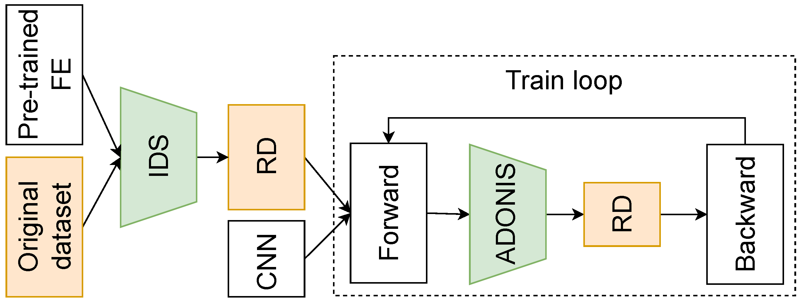
Figure 1. The proposed methods in the context of CNN training. The proposed methods are marked with green: IDS stands for Intellectual Data Selection, ADONIS denotes Adaptive Online Importance Sampling. Full and reduced datasets are marked in orange. Overall training acceleration methodology is as follows. First, a full training dataset is provided to IDS, which builds a sorted registry of samples based on a pre-trained feature extractor (FE). This happens before training at the so-called offline stage. Based on this index, the full dataset is reduced (reduced dataset, RD). Second, during CNN training (online stage) ADONIS further reduces a dataset by selecting samples based on losses information, thus producing a second version of RD. As a result, data are reduced up to 5×.
Mathematics 11 03120 g001
Figure 2. ADONIS. Updating the loss history with next the forward batch. The gray color stands for loss values that are dropped from history, the black color denotes samples that remain in history, and the red color designates new losses from forward batch that are added to history.
Mathematics 11 03120 g002
Figure 3. ADONIS. Clipping losses frequency histogram regarding σ . The violet color denotes samples that are clipped, and the orange color signifies losses that remain unchanged.
Mathematics 11 03120 g003
Figure 4. ADONIS. Identifying candidates for selection regarding θ . The green color highlights bins of losses that will be used for filtering, and the yellow color marks bins that do not satisfy the threshold criterion.
Mathematics 11 03120 g004
Figure 5. ADONIS. Selecting samples from forward batch regarding α . Blue color symbolizes rejected samples, red color indicates selected samples.
Mathematics 11 03120 g005
Figure 6. IDS. Selection of samples from CIFAR-100 based on pre-trained feature extractor (ResNet18). In (b): the cyan color denotes selected samples, the orange color signifies rejected samples, and the black triangle stands for class prototype.
Mathematics 11 03120 g006
Figure 7. Comparison of validation accuracy trajectories during ResNet18 training on CIFAR-100. Black - Default baseline full training. Experiments data, including ResNet50, MobileNet v2, YOLO v5 is presented in Table A1.
Mathematics 11 03120 g007
Figure 8. Samples selectivity analysis for IDS, ADONIS and SSP. (a) IDS. Samples from class #58 (pear) after K-Means clustering. (b) SSP. Samples from class #58 (pear) after SSP. (c) ADONIS. Most and least frequently selected samples from class #58 (pear). (d) ADONIS. Most and least frequently selected samples from the whole training dataset. In (a,b): the first row contains images that are the closest to the centroid. The second row contains images that are the most remote from the centroid. The class prototype is the leftmost image. In (c,d): the first row contains images that are the least frequently selected. The second row contains images that are the most frequently selected.
Mathematics 11 03120 g008aMathematics 11 03120 g008b
Figure 9. Comparison of validation accuracy trajectories during training YOLO v5 on MS COCO 2017.
Mathematics 11 03120 g009
Table 1. Evaluation of baseline training.
ModelDatasetAcc.Train
Time, s
ResNet18CIFAR-1095.092518
CIFAR-10076.432540
ImageNet 201270.0255,943
ResNet50CIFAR-1095.15913
CIFAR-10079.065910
ImageNet 201275.6153,409
MobileNet v2CIFAR-1090.894074
CIFAR-10068.264173
ImageNet 201268.0494,470
YOLO v5MS COCO 201742.55110,581
Disclaimer/Publisher’s Note: The statements, opinions and data contained in all publications are solely those of the individual author(s) and contributor(s) and not of MDPI and/or the editor(s). MDPI and/or the editor(s) disclaim responsibility for any injury to people or property resulting from any ideas, methods, instructions or products referred to in the content.