An Effective Approach Based on Generalized Bernstein Basis Functions for the System of Fourth-Order Initial Value Problems for an Arbitrary Interval

Abstract

The system of ordinary differential equations has many uses in contemporary mathematics and engineering. Finding the numerical solution to a system of ordinary differential equations for any arbitrary interval is very appealing to researchers. The numerical solution of a system of fourth-order ordinary differential equations on any finite interval $[a,b]$ is found in this work using a symmetric Bernstein approximation. This technique is based on the operational matrices of Bernstein polynomials for solving the system of fourth-order ODEs. First, using Chebyshev collocation nodes, a generalised approximation of the system of ordinary differential equations is discretized into a system of linear algebraic equations that can be solved using any standard rule, such as Gaussian elimination. We obtain the numerical solution in the form of a polynomial after obtaining the unknowns. The Hyers–Ulam and Hyers–Ulam–Rassias stability analyses are provided to demonstrate that the proposed technique is stable under certain conditions. The results of numerical experiments using the proposed technique are plotted in figures to demonstrate the accuracy of the specified approach. The results show that the suggested Bernstein approximation method for any interval is quick and effective.

1. Introduction and Fundamental Concepts

Ordinary differential equations (ODEs) are the most powerful mathematical tools found in the physical sciences. Many topics in mathematics, physics, and engineering are related to linear and nonlinear ODEs or systems of ODEs. The series of problems in ODEs with initial and boundary conditions arises in experimental physics, numerical simulation approaches, and many other scientific fields, including engineering, signals processing, economics, and acoustics. Many researchers have used various techniques to find approximate solutions to systems of ODEs. For illustration, Mesady et al. [1] presented a Jafari transformation for a system of linear ODEs with medical applications. By using the Jafari transform, ODEs can be transformed into a series of algebraic equations. Higazy and Aggarwal [2] presented the Sawi transformation for systems of ODEs. Sawi transformations have been used to obtain the concentration of chemical reactions for different examples from physical chemistry. In [3], Ricky et al. proposed the neural ordinary differential equations. This technique is based on parameterizing the derivative of the hidden state rather than specifying a deep series of concealed layers. In [4], Brown and Biggs provided methods for solving the ODEs for unconstrained optimization, while Zadunaisky [5] proposed a numerical technique to find the errors in the numerical solutions for the system of ODEs. In order to solve stiff and non-stiff systems of ODEs, in [6] Linda presented automatic selection of methods, which provides a way of determining whether or not a problem can be addressed by a set of strategies suitable for stiff or non-stiff problems. In recent years, many methods based on numerical investigation of nonlinear moving boundary problems, temperature-dependent numerical studies, the solutions of the nonlinear regularized long wave equation, and the nonlinear sinh-Gordon model have been proposed to find numerical solutions of physical models [7,8,9,10,11]. In [12], Neuberger presented the steepest descent in Hilbert spaces for a general system of linear differential equations. To forecast traffic on a limited time scale based on evolutionary algorithms, Chen et al. [13] explained time series forecasting using a system of ODEs. Farshid [14] proposed a differential transform method for systems of ODEs. The main aim of this effort was to catch the exact solution when the solution is known in terms of series expansion. Biazer et al. [15] presented the solution of a system of ODEs using the Adomian decomposition method by converting the given system into a system of first-order ODEs. Kurnaz and Galip [16] presented a comprehensive discussion of solving a system of ODEs by adjusting the step size. Their method allows for control of the truncation error used in numerical methods. In view of the above literature, a very small number of attempts have been made to find the numerical solution of a system of ODEs, and there are no works as yet addressing ways to find the numerical solution of a fourth-order ODE on any finite interval $[a,b]$. In this paper, a new method for finding a numerical solution to a system of fourth-order ODEs on any given interval is developed. It is demonstrated that the suggested method works well and is suitable for solving a linear system of fourth-order ODEs. Additionally, while the Hyers–Ulam stability of ODEs has recently been studied [17,18,19,20], no stability analysis of a system of ODEs for any given arbitrary interval has yet been carried out. In this paper, a new method is presented for solving systems of linear and nonlinear fourth-order ODEs using operational matrices of generalised symmetric Bernstein polynomials. Furthermore, Hyers–Ulam and Hyers–Ulam–Rassias stability analyses are provided for a system of fourth-order ODEs on any finite interval.

2. Preliminaries

The system of fourth-order ODEs has the layout

$$\begin{array}{c}\hfill \left\{\begin{array}{c}{D}_{xxxx}{v}_1\left(x\right)=f(x,v_q,D_x{v}_q,D_{xx}{v}_q,D_{xxx}{v}_q),\hfill \\ D_{xxxx}{v}_2\left(x\right)=f(x,v_q,D_x{v}_q,D_{xx}{v}_q,D_{xxx}{v}_q),\hfill \\ ⋮⋮⋮\hfill \\ D_{xxxx}{v}_k\left(x\right)=f(x,v_q,D_x{v}_q,D_{xx}{v}_q,D_{xxx}{v}_q),\hfill \end{array}\right.\end{array}$$

(1)

for $a\le x\le b$ and $q=1,2,\dots ,k$, with the following initial conditions:

$$\begin{array}{c}\hfill \left\{\begin{array}{c}{v}_1\left(a\right)=a_1,v_1^{\prime }\left(a\right)=b_1,v_1^{\prime \prime }\left(a\right)=c_1,v_1^{\prime \prime \prime }\left(a\right)=d_1,\hfill \\ v_2\left(a\right)=a_2,v_2^{\prime }\left(a\right)=b_2,v_2^{\prime \prime }\left(a\right)=c_2,v_2^{\prime \prime \prime }\left(a\right)=d_2,\hfill \\ ⋮⋮⋮\hfill \\ v_k\left(a\right)=a_k,v_k^{\prime }\left(a\right)=b_k,v_k^{\prime \prime }\left(a\right)=c_k,v_k^{\prime \prime \prime }\left(a\right)=d_k.\hfill \end{array}\right.\end{array}$$

(2)

where $a_q$, $b_q$, $c_q$, and $d_q$ are the given constants for $q=1,2,\dots ,k$ and $D_{xxxx}$ shows the fourth-order derivative. The goal is to use all of these initial conditions to find functions $v_1\left(x\right)$, $v_2\left(x\right)$,…,$v_k\left(x\right)$ that satisfy the differential equations in (1). The Bernstein polynomial approximation of the function $v_q\left(x\right):[a,b]\to R$ is defined as

$$\begin{array}{c}\hfill B_p(v_q;x)=\sum _{i=0}^p{\alpha }_{q,i}{B}_{i,p}\left(x\right),q=1,2,\dots ,k,\end{array}$$

(3)

and $B_{i,p}\left(x\right)$ is defined as

$$\begin{array}{c}\hfill B_{i,p}\left(v\right)={}^p{C}_i\frac{{(v-a)}^i{(b-v)}^{p-i}}{{(b-a)}^p},i=0,\dots ,p,\end{array}$$

(4)

where ${}^p{C}_i=\frac{p!}{i!(p-i)!}$, p is the degree, and i is an index of the Bernstein basis polynomial. Each Bernstein basis function satisfies the symmetry condition as follows:

$$\begin{array}{c}\hfill B_{i,p}\left(v\right)=B_{i-p,i}(a+b-v).\end{array}$$

The Bernstein basis function is non-negative, forms the partition of unity, and can be written in terms of power basis. The following result shows the convergence of Bernstein`s approximation for the system of ODEs.

Theorem 1.

Let $B_p(v_q;x)$ be the Bernstein polynomial approximation defined in Equation (3) and the sequence $\left\{B_p(v_q;x)\right\}$ for $q=1,2,\dots ,k$ converge to $v_q\left(x\right)$ for any $v_q\left(x\right)\in C[a,b]$.

Proof. 

See [21]. □

From Theorem 1, we is apparent that, for uniform continuity, for any $v_q\left(x\right)\in C[a,b]$ and for $ϵ>0$ there is an approximate solution $B_p(v_q;x)$ such that

$$\begin{array}{c}\hfill \parallel B_p(v_q;x)-v_q\left(x\right)\parallel <ϵ.\end{array}$$

(5)

In [22], it is proven that the degree of the polynomial p must satisfy the inequality $p>\frac{\mathrm{Ł}}{{\delta }^2ϵ}(a+b)(2-a-b)$, where $\mathrm{Ł}=\parallel v_q\parallel$.

3. The Numerical Scheme

In this section, the discretization technique for finding the solution of the system of fourth-order ODEs is presented. Here, the unknown function ${\alpha }_{q,i}$ is replaced by the Bernstein basis function from Equation (3), then the given system of ordinary differential equations is discretized using Chebyshev nodes.

Decomposition of Fourth-Order Ordinary Differential Equations

Linear combination of Bernstein basis functions $B_{p,i}\left(x\right)$, $i=0,1,2,\dots ,p$ of degree p yields the approximate polynomial $v^{\left[A\right]}\left(x\right)$ of the exact function $v\left(x\right)$, as follows:

$$\begin{array}{c}\hfill v^{\left[A\right]}\left(x\right)=\sum _{i=0}^p{\alpha }_i{B}_{i,p}\left(x\right)=D\psi \left(x\right),\end{array}$$

(6)

where $D=[{\alpha }_0,{\alpha }_1,...,{\alpha }_p]$ and $\psi \left(x\right)$= ${[B_{0,p},B_{1,p},...,B_{p,p}]}^T$, such as

$$\begin{array}{c}\hfill \psi \left(x\right)=\left[\begin{array}{c}\left(\genfrac{}{}{0pt}{}{p}{0}\right){(x-a)}^0{(b-x)}^{p-0}\\ \left(\genfrac{}{}{0pt}{}{p}{1}\right){(x-a)}^1{(b-x)}^{p-1}\\ ⋮& \\ \left(\genfrac{}{}{0pt}{}{p}{p}\right){(x-a)}^p{(b-x)}^0\end{array}\right].\end{array}$$

Now, the vector $\psi \left(x\right)$ can be expressed as a product of the matrix $(p+1)\times (p+1)$ and a vector $(p+1)\times 1$ as

$$\psi \left(x\right)=BX,$$

(7)

where

$$B=\frac{1}{{(b-a)}^p}\left[\begin{array}{ccccc}{a}_{00}& a_{01}& a_{02}& \cdots & a_{0p}\\ a_{10}& a_{11}& a_{12}& \cdots & a_{1p}\\ ⋮& ⋮& ⋮& \ddots \\ a_{p0}& a_{p1}& a_{p2}& \cdots & a_{pp}\end{array}\right],X=\left[\begin{array}{c}1\\ x\\ x^2\\ ⋮\\ x^p\end{array}\right].$$

(8)

Equation (7) implies that

$$\begin{array}{c}\hfill X=B^{-1}\psi \left(x\right),\end{array}$$

(9)

which can be solved using any standard rule (LU-method). The method for obtaining an approximate approach to the system of fourth-order ordinary differential equations is now presented. Consider $v_q^{\left[A\right]}\left(x\right)$ as an approximation of the qth function, provided as

$$\begin{array}{c}\hfill v_q^{\left[A\right]}\left(x\right)=\sum _{i=0}^p{\alpha }_{q,i}{B}_{i,p}\left(x\right)=D_q\psi \left(x\right),q=1,2,\dots ,k,\end{array}$$

where $D_q=[{\alpha }_{q,0},{\alpha }_{q,1},\dots ,{\alpha }_{q,p}]$. The derivative of $\psi \left(x\right)$ is denoted by $E^{{}^{\prime }}$, which is the $(p+1)\times (p+1)$ operational matrix, and $X={\left[1,x,x^2,\dots ,x^p\right]}^T$. This can be represented as follows:

$$\begin{array}{ccc}\hfill D_x\psi \left(x\right)=E^{{}^{\prime }}\psi \left(x\right)=B{D}_{x}X& =& B{D}_x\left[\begin{array}{c}1\\ x\\ x^2\\ ⋮\\ x^p\end{array}\right]\hfill \end{array}$$

$$\begin{array}{ccc}& =& B\left[\begin{array}{c}0\\ 1\\ 2x\\ ⋮\\ p{x}^{p-1}\end{array}\right]\hfill \\ & =& B\left[\begin{array}{ccccc}0& 0& 0& \cdots & 0\\ 1& 0& 0& \cdots & 0\\ 0& 2& 0& \cdots & 0\\ ⋮& \ddots & \ddots & \ddots & ⋮\\ 0& 0& \cdots & p& 0\end{array}\right]\left[\begin{array}{c}1\\ x\\ x^2\\ ⋮\\ x^{p-1}\\ x^p\end{array}\right]\hfill \\ & =& B\left[\begin{array}{ccccc}0& 0& 0& \cdots & 0\\ 1& 0& 0& \cdots & 0\\ 0& 2& 0& \cdots & 0\\ ⋮& \ddots & \ddots & \ddots & ⋮\\ 0& 0& \cdots & p& 0\end{array}\right]X.\hfill \end{array}$$

(10)

From (9), we have

$$\begin{array}{c}\hfill D_x\psi \left(x\right)=B\left[\begin{array}{ccccc}0& 0& 0& \cdots & 0\\ 1& 0& 0& \cdots & 0\\ 0& 2& 0& \cdots & 0\\ ⋮& \ddots & \ddots & \ddots & ⋮\\ 0& 0& \cdots & p& 0\end{array}\right]B^{-1}\psi \left(x\right).\end{array}$$

This implies that

$$\begin{array}{ccc}\hfill D_x& =& B\left[\begin{array}{ccccc}0& 0& 0& \cdots & 0\\ 1& 0& 0& \cdots & 0\\ 0& 2& 0& \cdots & 0\\ ⋮& \ddots & \ddots & \ddots & ⋮\\ 0& 0& \cdots & p& 0\end{array}\right]B^{-1},\hfill \\ & =& B\sigma B^{-1}\hfill \end{array}$$

where

$$\begin{array}{c}\hfill \sigma =\left[\begin{array}{ccccc}0& 0& 0& \cdots & 0\\ 1& 0& 0& \cdots & 0\\ 0& 2& 0& \cdots & 0\\ ⋮& \ddots & \ddots & \ddots & ⋮\\ 0& 0& \cdots & p& 0\end{array}\right].\end{array}$$

(11)

To solve the system of ODEs (1) using operational matrices, $v_q\left(x\right)$ can be approximated by the symmetric Bernstein polynomial as $v_q\left(x\right)=D_q\psi \left(x\right)$ along with

$$\begin{array}{ccc}\hfill D_x{v}_q\left(x\right)& =& D_q{E}^{\prime }\psi \left(x\right),\hfill \\ \hfill D_{xx}{v}_q\left(x\right)& =& D_q{\left(E^{\prime }\right)}^2\psi \left(x\right),\hfill \\ \hfill D_{xxx}{v}_q\left(x\right)& =& D_q{\left(E^{\prime }\right)}^3\psi \left(x\right).\hfill \end{array}$$

As a result, system (1) can be written as

$$\begin{array}{c}\hfill \left\{\begin{array}{c}{D}_1{\left(E^{\prime }\right)}^4\psi \left(x\right)=f(x,D_q\psi \left(x\right),D_q{E}^{\prime }\psi \left(x\right),D_q{\left(E^{\prime }\right)}^2\psi \left(x\right),D_q{\left(E^{\prime }\right)}^3\psi \left(x\right)),\hfill \\ D_2{\left(E^{\prime }\right)}^4\psi \left(x\right)=f(x,D_q\psi \left(x\right),D_q{E}^{\prime }\psi \left(x\right),D_q{\left(E^{\prime }\right)}^2\psi \left(x\right),D_q{\left(E^{\prime }\right)}^3\psi \left(x\right)),\hfill \\ ⋮⋮⋮⋮\hfill \\ D_k{\left(E^{\prime }\right)}^4\psi \left(x\right)=f(x,D_q\psi \left(x\right),D_q{E}^{\prime }\psi \left(x\right),D_q{\left(E^{\prime }\right)}^2\psi \left(x\right),D_q{\left(E^{\prime }\right)}^3\psi \left(x\right)),\hfill \end{array}\right.\end{array}$$

(12)

with the initial conditions

$$\begin{array}{c}\hfill \left\{\begin{array}{c}{D}_1\psi \left(a\right)=a_1,D_1{E}^{\prime }\psi \left(a\right)=b_1,D_1{\left(E^{\prime }\right)}^2\psi \left(a\right)=c_1,D_1{\left(E^{\prime }\right)}^3\psi \left(a\right)=d_1,\hfill \\ D_2\psi \left(a\right)=a_2,D_2{E}^{\prime }\psi \left(a\right)=b_2,D_2{\left(E^{\prime }\right)}^2\psi \left(a\right)=c_2,D_2{\left(E^{\prime }\right)}^3\psi \left(a\right)=d_2,\hfill \\ ⋮⋮⋮⋮\hfill \\ D_k\psi \left(a\right)=a_k,D_k{E}^{\prime }\psi \left(a\right)=b_k,D_k{\left(E^{\prime }\right)}^2\psi \left(a\right)=c_k,D_k{\left(E^{\prime }\right)}^3\psi \left(a\right)=d_k.\hfill \end{array}\right.\end{array}$$

(13)

Now, we substitute the collocation points in Equations (12) and (13) to obtain an algebraic equation system that can be solved easily. The collocation points in this case are the Chebyshev nodes, which are provided as

$$\begin{array}{c}\hfill x_{\beta }=\frac{1}{2}(a+b)+\frac{1}{2}(b-a)cos\left(\frac{(2\beta -1)\pi }{2p}\right),\beta =1,2,\cdots ,p-3.\end{array}$$

(14)

The Chebyshev nodes are very important in approximation, as they form a particularly good set of nodes for polynomial approximation.

4. Hyers–Ulam Stability

The study of stability problems for various functional equations is very important and has attracted the attention of many researchers. The definition of Hyers–Ulam stability has applicable significance, as it means that when studying the Hyers–Ulam stable system one does not have to reach the exact solution, which is often quite difficult or time-consuming. This is useful in many applications, for example fluid dynamics, numerical analysis, optimization, economics, etc. In this section, we examine the Hyers–Ulam stability and Hyers–Ulam–Rassias stability of the system of linear differential equations of order four, for which we consider the qth differential of system (1)

$$\begin{array}{c}\hfill v_q^{\left(iv\right)}\left(x\right)-\sum _{r=0}^3{a}_r\left(x\right)v_q^{\left(r\right)}\left(x\right)=0,q=1,2,\dots ,k,\end{array}$$

(15)

with the initial conditions

$$\begin{array}{c}\hfill v_q\left(a\right)=a_q,v_q^{\prime }\left(a\right)=b_q,v_q^{\prime \prime }\left(a\right)=c_{q}and{v}_q^{\prime \prime \prime }\left(a\right)=d_q\end{array}$$

(16)

for all $x\in I$, $v_q\left(x\right)\in C^4\left(I\right)$, and $I=[a,b]\subseteq \mathbf{R}$.

First, we provide definitions of Hyers–Ulam–Rassias stability and Hyers–Ulam stability for the qth differential (Equation (15)) with initial conditions (Equation (16)).

Definition 1

([23]). The system of fourth-order differential equations (Equation (15)) possesses Hyers–Ulam stability with the starting conditions in Equation (16) if a constant $M>0$ exists such that $x\in C^4\left(I\right)$ for each $ϵ>0$ if

$$\begin{array}{c}\hfill |v_q^{\left(iv\right)}\left(x\right)-\sum _{r=0}^3{a}_r\left(x\right)v_q^{\left(r\right)}\left(x\right)|\le ϵ,x\in I\end{array}$$

(17)

with initial conditions

$$\begin{array}{c}\hfill v_q\left(a\right)=a_q,v_q^{\prime }\left(a\right)=b_q,v_q^{\prime \prime }\left(a\right)=c_{q}and{v}_q^{\prime \prime \prime }\left(a\right)=d_q.\end{array}$$

(18)

Then, for each approximate solution at the pth degree $B_p(v_q;x)\in C^4\left(I\right)$ satisfying the differential equation (Equation (15)) with Equation (16), we have

$$\begin{array}{c}\hfill |v_q\left(x\right)-B_p(v_q;x)|\le Mϵ\forall x\in I,\end{array}$$

where a real number (M) is the Hyers–Ulam stability constant for the differential equation (Equation (15)) with Equation (16).

Definition 2

([23]). The system of the differential equation in Equation (15) possesses Hyers–Ulam–Rassias stability with the starting conditions in Equation (16) if $\varphi \left(x\right)\in C(I,{\mathbf{R}}_{+})$ such that $x\in C^4\left(I\right)$ for every $ϵ>0$ if

$$\begin{array}{c}\hfill |v_q^{\left(iv\right)}\left(x\right)-\sum _{r=0}^3{a}_r\left(x\right)v_q^{\left(r\right)}\left(x\right)|\le ϵ\varphi \left(x\right),x\in I\end{array}$$

(19)

with initial conditions

$$\begin{array}{c}\hfill v_q\left(a\right)=a_q,v_q^{\prime }\left(a\right)=b_q,v_q^{\prime \prime }\left(a\right)=c_{q}and{v}_q^{\prime \prime \prime }\left(a\right)=d_q.\end{array}$$

(20)

Then, for each approximate solution at the pth degree $B_p(v_q;x)\in C^4\left(I\right)$ satisfying the differential equation (Equation (15)) with Equation (16), we have

$$\begin{array}{c}\hfill |v_q\left(x\right)-B_p(v_q;x)|\le Mϵ\varphi \left(x\right)\forall x\in I,\end{array}$$

where a real number (M) is the Hyers–Ulam–Rassias stability constant for the differential equation (Equation (15)) with Equation (16).

The following main results provide the Hyers–Ulam–Rassias stability and Hyers–Ulam stability of the system of differential equations ( Equation (15)) with Equation (16).

Theorem 2.

If ${\sum }_{r=0}^{3}max|a_r\left(x\right)|<\frac{4!}{{(b-a)}^4}$, then the system of differential equations (Equation (1)) has Hyers–Ulam stability with the initial conditions in Equation (2).

Proof. 

For every $ϵ>0$, consider

$$\begin{array}{c}\hfill |v_q^{\left(iv\right)}\left(x\right)-\sum _{r=0}^3{a}_r\left(x\right)v_q^{\left(r\right)}\left(x\right)|<ϵ\end{array}$$

(21)

with initial conditions

$$\begin{array}{c}\hfill v_q\left(a\right)=a_q,v_q^{\prime }\left(a\right)=b_q,v_q^{\prime \prime }\left(a\right)=c_{q}and{v}_q^{\prime \prime \prime }\left(a\right)=d_q.\end{array}$$

Here, $v_q\left(x\right)\in C^4\left([a,b]\right)$ satisfies $|v_q^{\prime \prime \prime }\left(x\right)|<|v_q^{\prime \prime }\left(x\right)|<|v_q^{\prime }\left(x\right)|<|v_q\left(x\right)|$; thus, per Taylor’s formula, we have

$$\begin{array}{c}\hfill v_q\left(x\right)=v_q\left(a\right)+v_q^{\prime }\left(a\right)(x-a)+v_q^{\prime \prime }\left(a\right)\frac{{(x-a)}^2}{2!}+v_q^{\prime \prime \prime }\left(a\right)\frac{{(x-a)}^3}{3!}+v_q^{\left(iv\right)}\left(\xi \right)\frac{{(x-a)}^4}{4!}.\end{array}$$

Thus,

$$\begin{array}{c}\hfill |v_q\left(x\right)|=|v_q\left(a\right)+v_q^{\prime }\left(a\right)(x-a)+v_q^{\prime \prime }\left(a\right)\frac{{(x-a)}^2}{2!}+v_q^{\prime \prime \prime }\left(a\right)\frac{{(x-a)}^3}{3!}+v_q^{\left(iv\right)}\left(\xi \right)\frac{{(x-a)}^4}{4!}|,\end{array}$$

which implies that

$$\begin{array}{c}\hfill max|v_q\left(x\right)|\le \left\{1+(b-a)+\frac{{(b-a)}^2}{2!}+\frac{{(b-a)}^3}{3!}\right\}max|v_q\left(x\right)|+\frac{{(b-a)}^4}{4!}max|v_q^{\left(iv\right)}\left(x\right)|,\end{array}$$

in turn implying that

$$\begin{array}{c}\hfill max|v_q\left(x\right)|=\eta max|v_q\left(x\right)|+\frac{{(b-a)}^4}{4!}\left\{max|v_q^{\left(iv\right)}\left(x\right)-\sum _{r=0}^3{a}_r\left(x\right)v_q^{\left(r\right)}\left(x\right)+\sum _{r=0}^3{a}_r\left(x\right)v_q^{\left(r\right)}\left(x\right)|\right\},\end{array}$$

where $\eta =1+(b-a)+\frac{{(b-a)}^2}{2!}+\frac{{(b-a)}^3}{3!}$. From Equation (21), we have

$$\begin{array}{ccc}\hfill max|v_q\left(x\right)|& \le & \eta max|v_q\left(x\right)|+\frac{{(b-a)}^4}{4!}\left\{ϵ+\sum _{r=0}^3{a}_r\left(x\right)max|v_q\left(x\right)|\right\}\hfill \\ & =& \left(\eta +\sum _{r=0}^3{a}_r\left(x\right)\frac{{(b-a)}^4}{4!}\right)max|v_q\left(x\right)|+\frac{{(b-a)}^4}{4!}ϵ\hfill \\ & =& \delta max|v_q\left(x\right)|+\frac{{(b-a)}^4}{4!}ϵ\hfill \end{array}$$

Finally,

$$\begin{array}{c}\hfill max|v_q\left(x\right)|\le \frac{{(b-a)}^4}{4!(1-\delta )}ϵ.\end{array}$$

Choosing M as $\frac{{(b-a)}^4}{4!(1-\delta )}$, where $\delta =\eta +{\sum }_{r=0}^3{a}_r\left(x\right)\frac{{(b-a)}^4}{4!}$, we have

$$max|v_q\left(x\right)|\le Mϵ.$$

Obviously, if $v_q^{\left[A\right]}\left(x\right)$ is the approximate solution of Equation (15) with Equation (16), then

$$\begin{array}{c}\hfill |v_q\left(x\right)-v_q^{\left[A\right]}\left(x\right)|\le Mϵ.\end{array}$$

□

As a result of Definition 1, the system of the fourth-order differential equation in Equation (1) is Hyers–Ulam stable.

Theorem 3.

If ${\sum }_{r=0}^{3}max|a_r\left(x\right)|<\frac{4!}{{(b-a)}^4}$, then the system of the ordinary differential equation in Equation (1) has Hyers–Ulam–Rassias stability with initial conditions Equation (2).

Proof. 

For every $ϵ>0$ and $\phi :[a,b]\to [0,\infty )$, consider

$$\begin{array}{c}\hfill |v_q^{\left(iv\right)}\left(x\right)-\sum _{r=0}^3{a}_r\left(x\right)v_q^{\left(r\right)}\left(x\right)|<\phi \left(x\right)ϵ\end{array}$$

(22)

with initial conditions

$$\begin{array}{c}\hfill v_q\left(a\right)=a_q,v_q^{\prime }\left(a\right)=b_q,v_q^{\prime \prime }\left(a\right)=c_{q}and{v}_q^{\prime \prime \prime }\left(a\right)=d_q.\end{array}$$

Here, $v_q\left(x\right)\in C^4\left([a,b]\right)$ satisfies $|v_q^{\prime \prime \prime }\left(x\right)|<|v_q^{\prime \prime }\left(x\right)|<|v_q^{\prime }\left(x\right)|<|v_q\left(x\right)|$; thus, per Taylor’s formula we have

$$\begin{array}{c}\hfill v_q\left(x\right)=v_q\left(a\right)+v_q^{\prime }\left(a\right)(x-a)+v_q^{\prime \prime }\left(a\right)\frac{{(x-a)}^2}{2!}+v_q^{\prime \prime \prime }\left(a\right)\frac{{(x-a)}^3}{3!}+v_q^{\left(iv\right)}\left(\xi \right)\frac{{(x-a)}^4}{4!},\end{array}$$

which implies that

$$\begin{array}{c}\hfill max|v_q\left(x\right)|\le \left\{1+(b-a)+\frac{{(b-a)}^2}{2!}+\frac{{(b-a)}^3}{3!}\right\}max|v_q\left(x\right)|+\frac{{(b-a)}^4}{4!}max|v_q^{\left(iv\right)}\left(x\right)|.\end{array}$$

Thus,

$$\begin{array}{ccc}\hfill max|v_q\left(x\right)|& \le & \eta max|v_q\left(x\right)|+\frac{{(b-a)}^4}{4!}\left\{\phi \left(x\right)ϵ+\sum _{r=0}^3{a}_r\left(x\right)max|v_q\left(x\right)|\right\}.\hfill \end{array}$$

Finally,

$$\begin{array}{c}\hfill max|v_q\left(x\right)|\le \frac{{(b-a)}^4}{4!(1-\delta )}\phi \left(x\right)ϵ.\end{array}$$

Obviously, if $v_q^{\left[A\right]}\left(x\right)$ is the approximate solution of Equation (15) with Equation (16), then

$$\begin{array}{c}\hfill |v_q\left(x\right)-v_q^{\left[A\right]}\left(x\right)|\le M\phi \left(x\right)ϵ,\end{array}$$

where $M=\frac{{(b-a)}^4}{4!(1-\delta )}$, $\delta =\eta +{\sum }_{r=0}^3{a}_r\left(x\right)\frac{{(b-a)}^4}{4!}$, and $\eta =1+(b-a)+\frac{{(b-a)}^2}{2!}+\frac{{(b-a)}^3}{3!}$. □

Thus, the system of fourth-order differential equations in Equation (1) exhibits Hyers–Ulam–Rassias stability as a result of Definition 2.

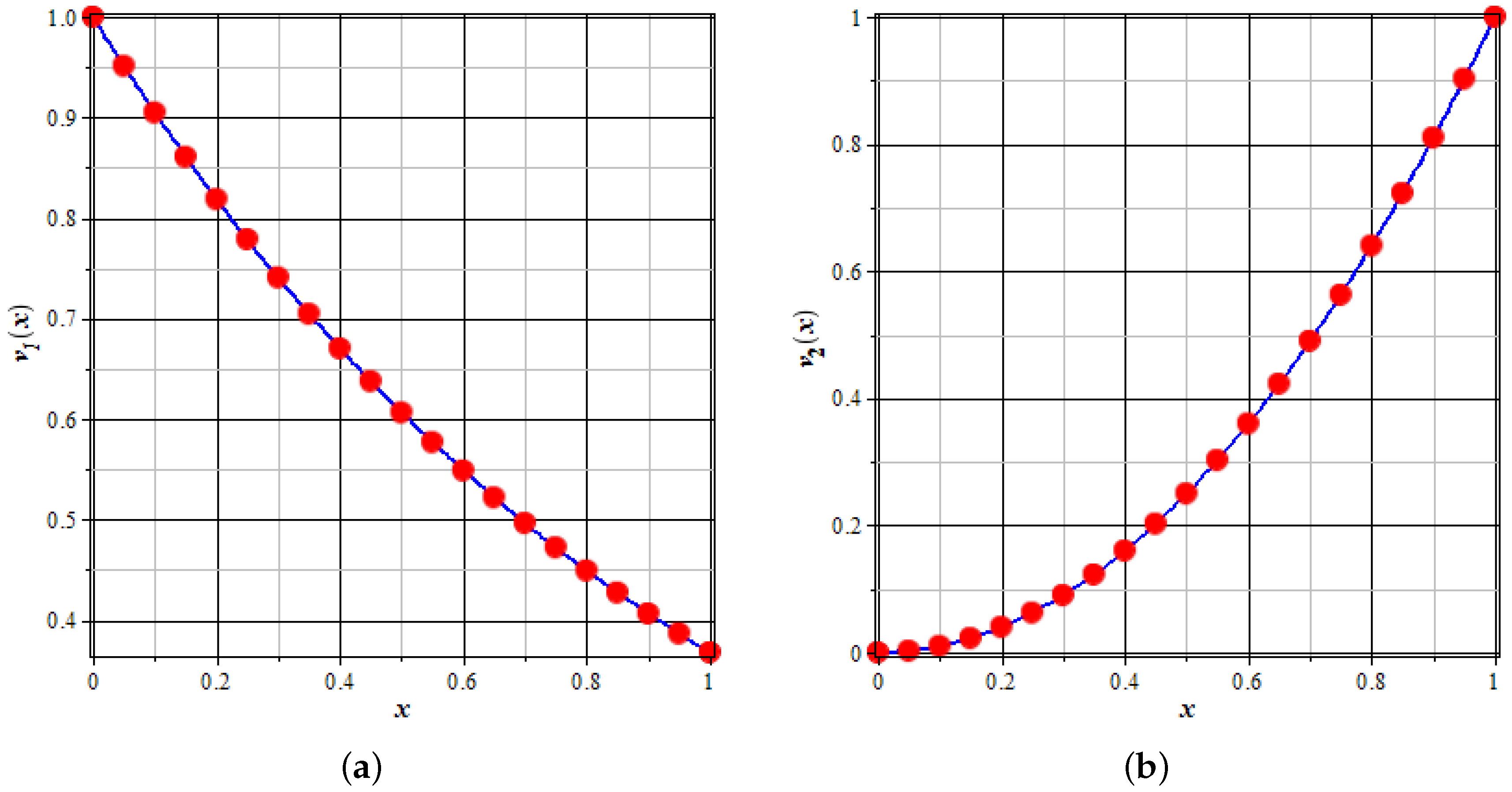
5. Numerical Problems

This portion considers a number of mathematical problems that can be solved utilizing numerical techniques depending on the symmetry of Bernstein’s polynomials. Table 1, Table 2, Table 3, Table 4, Table 5 and Table 6 demonstrate that the presented approach is both effective and accurate. Graphs are shown in Figure 1, Figure 2 and Figure 3 to demonstrate the actual and numerical solutions and compare their accuracy. The following formula is used to calculate the error at the pth degree:

$$\begin{array}{c}\hfill \parallel E_{q,p}\parallel =|v_q\left(x\right)-v_q^{\left[A\right]}\left(x\right)|,\end{array}$$

(23)

where $E_{q,p}$ is the error of the qth function, $v_q\left(x\right)$ is the exact solution, and $v_q^{\left[A\right]}\left(x\right)$ is the approximate solution. MAPLE and MATLAB computer languages were used on R2018a running on an Intel(R) Core(TM) i7-1165G7 CPU 1.30 GHz processor with 8.00 GB RAM to execute the numerical computations for the solution of numerical problems.

Table 1. Absolute error of the system in Equation (24) at distinct nodes between 0 and 1 for degree $p=6$ and $p=10$ of Bernstein basis polynomials.

x	${\mathit{E}}_{1,6}\left(\mathit{x}\right)$	${\mathit{E}}_{1,10}\left(\mathit{x}\right)$	${\mathit{E}}_{2,6}\left(\mathit{x}\right)$	${\mathit{E}}_{2,10}\left(\mathit{x}\right)$
$0.0$	$0.0$	$0.0$	$0.0$	$0.0$
$0.1$	$7.84\times {10}^{-8}$	$2.04\times {10}^{-12}$	$1.64\times {10}^{-9}$	$1.53\times {10}^{-16}$
$0.2$	$1.12\times {10}^{-8}$	$2.42\times {10}^{-11}$	$2.79\times {10}^{-7}$	$1.34\times {10}^{-13}$
$0.3$	$5.09\times {10}^{-6}$	$9.58\times {10}^{-11}$	$1.49\times {10}^{-7}$	$1.18\times {10}^{-12}$
$0.4$	$1.44\times {10}^{-6}$	$2.46\times {10}^{-10}$	$4.99\times {10}^{-7}$	$4.96\times {10}^{-12}$
$0.5$	$3.19\times {10}^{-5}$	$5.04\times {10}^{-10}$	$1.28\times {10}^{-6}$	$1.45\times {10}^{-11}$
$0.6$	$6.0\times {10}^{-5}$	$9.00\times {10}^{-10}$	$2.79\times {10}^{-6}$	$3.41\times {10}^{-11}$
$0.7$	$1.01\times {10}^{-5}$	$1.46\times {10}^{-9}$	$5.41\times {10}^{-6}$	$6.96\times {10}^{-11}$
$0.8$	$1.58\times {10}^{-4}$	$2.22\times {10}^{-9}$	$9.64\times {10}^{-6}$	$1.28\times {10}^{-10}$
$0.9$	$2.34\times {10}^{-4}$	$3.20\times {10}^{-9}$	$1.60\times {10}^{-5}$	$2.18\times {10}^{-10}$
1	$3.31\times {10}^{-4}$	$4.44\times {10}^{-9}$	$2.54\times {10}^{-5}$	$3.15\times {10}^{-10}$

Table 2. Relative error of the system in Equation (24) at distinct nodes between 0 and 1 for degree $p=6$ and $p=10$ of Bernstein basis polynomials.

x	${\mathit{E}}_{1,6}\left(\mathit{x}\right)$	${\mathit{E}}_{1,10}\left(\mathit{x}\right)$	${\mathit{E}}_{2,6}\left(\mathit{x}\right)$	${\mathit{E}}_{2,10}\left(\mathit{x}\right)$
$0.0$	$0.0$	$0.0$	$0.0$	$0.0$
$0.1$	$8.66\times {10}^{-8}$	$2.04\times {10}^{-10}$	$1.81\times {10}^{-9}$	$1.53\times {10}^{-14}$
$0.2$	$1.36\times {10}^{-8}$	$6.05\times {10}^{-11}$	$3.40\times {10}^{-7}$	$3.35\times {10}^{-12}$
$0.3$	$6.87\times {10}^{-6}$	$1.06\times {10}^{-9}$	$1.10\times {10}^{-7}$	$1.31\times {10}^{-11}$
$0.4$	$2.14\times {10}^{-6}$	$1.53\times {10}^{-9}$	$3.34\times {10}^{-7}$	$3.11\times {10}^{-11}$
$0.5$	$5.25\times {10}^{-6}$	$2.01\times {10}^{-9}$	$7.76\times {10}^{-7}$	$5.81\times {10}^{-11}$
$0.6$	$1.09\times {10}^{-4}$	$2.50\times {10}^{-9}$	$1.53\times {10}^{-6}$	$9.47\times {10}^{-11}$
$0.7$	$2.03\times {10}^{-5}$	$2.97\times {10}^{-9}$	$2.68\times {10}^{-6}$	$1.42\times {10}^{-10}$
$0.8$	$3.51\times {10}^{-4}$	$3.46\times {10}^{-9}$	$4.33\times {10}^{-6}$	$2.00\times {10}^{-10}$
$0.9$	$5.75\times {10}^{-4}$	$3.95\times {10}^{-9}$	$6.50\times {10}^{-6}$	$2.69\times {10}^{-10}$
1	$8.99\times {10}^{-4}$	$4.44\times {10}^{-9}$	$9.34\times {10}^{-6}$	$3.15\times {10}^{-10}$

Table 3. Absolute error of the system in Equation (25) at distinct nodes between 0 and 1 for degree $p=6$ and $p=10$ of Bernstein basis polynomials.

x	${\mathit{E}}_{1,6}\left(\mathit{x}\right)$	${\mathit{E}}_{1,10}\left(\mathit{x}\right)$	${\mathit{E}}_{2,6}\left(\mathit{x}\right)$	${\mathit{E}}_{2,10}\left(\mathit{x}\right)$
$0.0$	$0.0$	$0.0$	$0.0$	$0.0$
$0.1$	$5.14\times {10}^{-7}$	$2.16\times {10}^{-11}$	$1.04\times {10}^{-8}$	$2.89\times {10}^{-12}$
$0.2$	$7.36\times {10}^{-6}$	$2.57\times {10}^{-10}$	$1.51\times {10}^{-6}$	$3.47\times {10}^{-11}$
$0.3$	$3.34\times {10}^{-5}$	$1.01\times {10}^{-9}$	$6.98\times {10}^{-5}$	$1.39\times {10}^{-10}$
$0.4$	$9.50\times {10}^{-5}$	$2.61\times {10}^{-9}$	$2.20\times {10}^{-5}$	$3.66\times {10}^{-10}$
$0.5$	$2.09\times {10}^{-4}$	$5.35\times {10}^{-9}$	$4.54\times {10}^{-5}$	$7.74\times {10}^{-10}$
$0.6$	$3.94\times {10}^{-4}$	$9.56\times {10}^{-9}$	$8.75\times {10}^{-5}$	$1.43\times {10}^{-9}$
$0.7$	$6.68\times {10}^{-4}$	$1.55\times {10}^{-8}$	$1.51\times {10}^{-4}$	$2.42\times {10}^{-9}$
$0.8$	$1.04\times {10}^{-3}$	$2.36\times {10}^{-8}$	$2.44\times {10}^{-4}$	$3.85\times {10}^{-9}$
$0.9$	$1.54\times {10}^{-3}$	$3.41\times {10}^{-8}$	$3.73\times {10}^{-4}$	$5.83\times {10}^{-9}$
1	$2.19\times {10}^{-3}$	$4.75\times {10}^{-8}$	$5.46\times {10}^{-4}$	$8.53\times {10}^{-9}$

Table 4. Relative error of the system in Equation (25) at distinct nodes between 0 and 1 for degree $p=6$ and $p=10$ of Bernstein basis polynomials.

x	${\mathit{E}}_{1,6}\left(\mathit{x}\right)$	${\mathit{E}}_{1,10}\left(\mathit{x}\right)$	${\mathit{E}}_{2,6}\left(\mathit{x}\right)$	${\mathit{E}}_{2,10}\left(\mathit{x}\right)$
$0.0$	$0.0$	$0.0$	$0.0$	$0.0$
$0.1$	$4.49\times {10}^{-6}$	$1.56\times {10}^{-10}$	$4.32\times {10}^{-6}$	$9.94\times {10}^{-9}$
$0.2$	$1.50\times {10}^{-5}$	$4.54\times {10}^{-9}$	$1.33\times {10}^{-4}$	$2.65\times {10}^{-9}$
$0.3$	$3.54\times {10}^{-4}$	$9.73\times {10}^{-9}$	$3.15\times {10}^{-2}$	$5.24\times {10}^{-8}$
$0.4$	$3.54\times {10}^{-4}$	$9.73\times {10}^{-9}$	$3.15\times {10}^{-3}$	$5.24\times {10}^{-8}$
$0.5$	$6.89\times {10}^{-4}$	$1.76\times {10}^{-8}$	$5.20\times {10}^{-3}$	$8.86\times {10}^{-8}$
$0.6$	$1.19\times {10}^{-3}$	$2.90\times {10}^{-8}$	$8.35\times {10}^{-3}$	$1.36\times {10}^{-7}$
$0.7$	$1.92\times {10}^{-3}$	$4.45\times {10}^{-8}$	$1.23\times {10}^{-2}$	$1.98\times {10}^{-7}$
$0.8$	$2.89\times {10}^{-3}$	$6.56\times {10}^{-8}$	$1.74\times {10}^{-2}$	$2.75\times {10}^{-7}$
$0.9$	$4.20\times {10}^{-3}$	$9.31\times {10}^{-8}$	$2.37\times {10}^{-2}$	$3.71\times {10}^{-7}$
1	$2.19\times {10}^{-3}$	$4.75\times {10}^{-8}$	$3.12\times {10}^{-2}$	$4.88\times {10}^{-7}$

Table 5. Absolute error of the system in Equation (26) at distinct nodes between 0 and 1 for degree $p=6$ and $p=10$ of Bernstein basis polynomials.

x	${\mathit{E}}_{1,6}\left(\mathit{x}\right)$	${\mathit{E}}_{1,10}\left(\mathit{x}\right)$	${\mathit{E}}_{2,6}\left(\mathit{x}\right)$	${\mathit{E}}_{2,10}\left(\mathit{x}\right)$
$0.0$	$0.0$	$0.0$	$0.0$	$0.0$
$0.1$	$7.46\times {10}^{-7}$	$3.15\times {10}^{-11}$	$1.89\times {10}^{-8}$	$4.11\times {10}^{-13}$
$0.2$	$1.07\times {10}^{-5}$	$3.75\times {10}^{-10}$	$2.75\times {10}^{-7}$	$4.94\times {10}^{-12}$
$0.3$	$4.87\times {10}^{-5}$	$1.48\times {10}^{-9}$	$1.26\times {10}^{-6}$	$1.97\times {10}^{-11}$
$0.4$	$1.38\times {10}^{-4}$	$3.81\times {10}^{-9}$	$3.65\times {10}^{-6}$	$5.14\times {10}^{-11}$
$0.5$	$3.06\times {10}^{-4}$	$7.81\times {10}^{-9}$	$8.20\times {10}^{-6}$	$1.08\times {10}^{-10}$
$0.6$	$5.77\times {10}^{-4}$	$1.39\times {10}^{-9}$	$1.57\times {10}^{-5}$	$2.00\times {10}^{-10}$
$0.7$	$9.77\times {10}^{-4}$	$2.27\times {10}^{-9}$	$2.73\times {10}^{-5}$	$3.43\times {10}^{-10}$
$0.8$	$1.53\times {10}^{-3}$	$3.45\times {10}^{-8}$	$4.43\times {10}^{-5}$	$5.06\times {10}^{-10}$
$0.9$	$2.26\times {10}^{-3}$	$4.98\times {10}^{-8}$	$6.85\times {10}^{-5}$	$8.85\times {10}^{-10}$
1	$3.20\times {10}^{-3}$	$6.91\times {10}^{-8}$	$1.02\times {10}^{-4}$	$1.36\times {10}^{-9}$

Table 6. Relative error of the system in Equation (26) at distinct nodes between 0 and 1 for degree $p=6$ and $p=10$ of Bernstein basis polynomials.

x	${\mathit{E}}_{1,6}\left(\mathit{x}\right)$	${\mathit{E}}_{1,10}\left(\mathit{x}\right)$	${\mathit{E}}_{2,6}\left(\mathit{x}\right)$	${\mathit{E}}_{2,10}\left(\mathit{x}\right)$
$0.0$	$0.0$	$0.0$	$0.0$	$0.0$
$0.1$	$7.46\times {10}^{-6}$	$3.15\times {10}^{-10}$	$1.71\times {10}^{-7}$	$3.73\times {10}^{-12}$
$0.2$	$5.35\times {10}^{-5}$	$1.87\times {10}^{-9}$	$1.14\times {10}^{-6}$	$2.05\times {10}^{-11}$
$0.3$	$1.62\times {10}^{-4}$	$3.7\times {10}^{-9}$	$3.23\times {10}^{-6}$	$5.05\times {10}^{-11}$
$0.4$	$3.45\times {10}^{-4}$	$9.52\times {10}^{-9}$	$3.65\times {10}^{-6}$	$9.17\times {10}^{-11}$
$0.5$	$6.12\times {10}^{-4}$	$1.56\times {10}^{-9}$	$1.09\times {10}^{-5}$	$1.44\times {10}^{-10}$
$0.6$	$9.61\times {10}^{-4}$	$2.31\times {10}^{-9}$	$1.63\times {10}^{-5}$	$2.08\times {10}^{-10}$
$0.7$	$1.39\times {10}^{-3}$	$3.24\times {10}^{-9}$	$2.29\times {10}^{-5}$	$2.88\times {10}^{-10}$
$0.8$	$1.91\times {10}^{-3}$	$4.31\times {10}^{-8}$	$3.07\times {10}^{-5}$	$3.51\times {10}^{-10}$
$0.9$	$2.51\times {10}^{-3}$	$5.53\times {10}^{-8}$	$4.00\times {10}^{-5}$	$5.17\times {10}^{-10}$
1	$3.20\times {10}^{-3}$	$6.91\times {10}^{-8}$	$5.10\times {10}^{-4}$	$6.8\times {10}^{-10}$

Figure 1. Comparison of numerical and exact results of $v_1\left(x\right)$ in (a) and $v_2\left(x\right)$ in (b) for degree $p=10$ at distinct node points $x\in [0,1]$ of Problem 1.

Figure 2. Comparison of numerical and exact results of $v_1\left(x\right)$ in (a) and $v_2\left(x\right)$ in (b) for degree $p=10$ at distinct node points $x\in [0,1]$ of Problem 2.

Figure 3. Comparison of numerical and exact results of $v_1\left(x\right)$ in (a) and $v_2\left(x\right)$ in (b) for degree $p=10$ at distinct node points $x\in [0,1]$ of Problem 3.

Problem 1.

Consider the following system of fourth-order ordinary differential equations arising in beam-column theory:

$$\begin{array}{ccc}\hfill & & e^{2x}\frac{d^4{v}_1}{d{x}^4}+\frac{d{v}_2}{dx}=2x+e^x,\hfill \\ & & sin{x}^2\frac{d^4{v}_2}{d{x}^4}+\frac{d{v}_1}{dx}=-e^{-x},\hfill \end{array}$$

(24)

subject to initial conditions

$$\begin{array}{ccc}& & v_1\left(0\right)=1,v_1^{\prime }\left(0\right)=-1,v_1^{\prime \prime }\left(0\right)=1,v_1^{\prime \prime \prime }\left(0\right)=-1,\hfill \\ & & v_2\left(0\right)=0,v_2^{\prime }\left(0\right)=0,v_2^{\prime \prime }\left(0\right)=2,v_2^{\prime \prime \prime }\left(0\right)=0,\hfill \end{array}$$

and with exact solutions

$$\begin{array}{c}\hfill v_1\left(x\right)=e^{-x},v_2\left(x\right)=x^2.\end{array}$$

Using the proposed technique described in Section 3, we obtain the following approximate solutions for degree $p=6$:

$$\begin{array}{ccc}\hfill v_{1,6}^{\left[A\right]}\left(x\right)& \approx & 0.000752383749x^6-0.00732584334x^5+0.0407880099x^4-0.1666x^3+0.5x^2-x+1.\hfill \\ \hfill v_{2,6}^{\left[A\right]}\left(x\right)& \approx & -0.000000368277456x^6+0.0000104695635x^5+0.0000153956102x^4+x^2.\hfill \end{array}$$

Similarly, the approximate solutions for degree $p=10$ are as follows:

$$\begin{array}{ccc}\hfill v_{1,10}^{\left[A\right]}\left(x\right)& \approx & 0.000000157599924x^{10}-0.000000246680218x^9+0.000024375981x^8-0.00019800899x^7\hfill \\ & & +0.00138863514x^6-0.00833322734x^5+0.0416666378x^4-0.1666666667x^3+0.5x^2-x+1.\hfill \\ \hfill v_{2,10}^{\left[A\right]}\left(x\right)& \approx & -0.00000000001x^{10}+0.0000000007x^9-0.000000001x^8+0.000000002x^7\hfill \\ & & -0.000000002x^6+0.000000001x^5-0.00000000001x^4+x^2.\hfill \end{array}$$

The respective absolute errors of these solutions for degree $p=6$ and $p=10$ are provided in Table 1. A comparison of these numerical results shows the effectiveness and fast convergence of the proposed technique.

Problem 2.

Consider the system of fourth-order ordinary differential equations:

$$\begin{array}{ccc}\hfill & & \frac{d^4{v}_1}{d{x}^4}+\frac{d^2{v}_2}{d{x}^2}=x{e}^{-x}-4e^{-x}-sinx,\hfill \\ & & \frac{d^4{v}_2}{d{x}^4}+\frac{d^2{v}_1}{d{x}^2}=sinx+x{e}^{-x}-2e^{-x},\hfill \end{array}$$

(25)

subject to initial conditions

$$\begin{array}{c}\hfill v_1\left(0\right)=0,v_1^{\prime }\left(0\right)=1,v_1^{\prime \prime }\left(0\right)=3,v_1^{\prime \prime \prime }\left(0\right)=-4,\\ \hfill v_2\left(0\right)=0,v_2^{\prime }\left(0\right)=1,v_2^{\prime \prime }\left(0\right)=0,v_2^{\prime \prime \prime }\left(0\right)=-1,\end{array}$$

and with exact solutions

$$\begin{array}{c}\hfill v_1\left(x\right)=x{e}^{-x},v_2\left(x\right)=sinx.\end{array}$$

Using the proposed technique described in Section 3, we obtain the following approximate solutions for degree $p=6$:

$$\begin{array}{ccc}\hfill v_{1,6}^{\left[A\right]}\left(x\right)& \approx & -0.00404440557x^6+0.0350125944x^5-0.160895381x^4+0.5x^3-x^2+x.\hfill \\ \hfill v_{2,6}^{\left[A\right]}\left(x\right)& \approx & -0.00080338704x^6+0.00955722545x^5-0.0011631606x^4-0.16x^3+x.\hfill \end{array}$$

Similarly, the approximate solutions for degree $p=10$ are as follows:

$$\begin{array}{ccc}\hfill v_{1,10}^{\left[A\right]}\left(x\right)& \approx & -0.0000014885022x^{10}+0.0000217261914x^9-0.000193901265x^8+0.00138461759x^7\hfill \\ & & -0.00833065013x^6+0.0416655459x^5-0.166666361x^4+0.50x^3-x^2+x.\hfill \\ \hfill v_{2,10}^{\left[A\right]}\left(x\right)& \approx & -1.0000000463173x^{10}+0.000003139404x^9-5.00000008280x^8-0.000197850635x^7\hfill \\ & & -3.00000056860x^6+0.00833348079x^5-4.0000000006391x^4-0.1666666667\ast x^3+x.\hfill \end{array}$$

Table 3 shows the respective absolute errors of these solutions for degrees $p=6$ and $p=10$. Comparing these numerical results demonstrates the proposed technique’s effectiveness and rapid convergence.

Problem 3.

Consider the following nonlinear system of fourth-order ordinary differential equations:

$$\begin{array}{ccc}\hfill & & x^2\frac{d^4{v}_1}{d{x}^4}+{sin}^{2}x\frac{d^3{v}_2}{d{x}^3}+\frac{d{v}_2}{dx}=4x^{2}sinx+x^{3}cosx+2x+1.0\le x\le 1,\hfill \\ & & {cos}^{-1}x\frac{d^4{v}_2}{d{x}^4}+x^2\frac{d^3{v}_2}{d{x}^3}+\frac{d{v}_1}{dx}=cosx-xsinx.\hfill \end{array}$$

(26)

subject to initial conditions

$$\begin{array}{ccc}& & v_1\left(0\right)=0,v_1^{\prime }\left(0\right)=1,v_1^{\prime \prime }\left(0\right)=0,v_1^{\prime \prime \prime }\left(0\right)=-3.\hfill \\ & & v_2\left(0\right)=0,v_2^{\prime }\left(0\right)=1,v_2^{\prime \prime }\left(0\right)=2,v_2^{\prime \prime \prime }\left(0\right)=0.\hfill \end{array}$$

and with exact solutions

$$\begin{array}{c}\hfill v_1\left(x\right)=xcosx,v_2\left(x\right)=x^2+x.\end{array}$$

Using the proposed technique described in Section 3, we obtain the following approximate solutions for degree $p=6$:

$$\begin{array}{ccc}\hfill v_{1,6}^{\left[A\right]}\left(x\right)& \approx & -0.0055108317x^6+0.0509503842x^5-0.00834103905x^4-0.5x^3+x.\hfill \\ \hfill v_{2,6}^{\left[A\right]}\left(x\right)& \approx & 0.0000989355488x^6-0.000205561024x^5+0.000209351273x^4+x^2+x.\hfill \end{array}$$

Similarly, the approximate solutions for degree $p=10$ are as follows:

$$\begin{array}{ccc}\hfill v_{1,10}^{\left[A\right]}\left(x\right)& \approx & -0.00000159494x^{10}+0.000028967068x^9-0.0000063157x^8-0.0013828025x^7\hfill \\ & & -0.000003863542x^6+0.0416682915x^5-4.0000000450508x^4-0.5x^3+x.\hfill \\ \hfill v_{2,10}^{\left[A\right]}\left(x\right)& \approx & 0.00000000476x^{10}-0.000000023321x^9+0.000000049280x^8-0.000000058259x^7\hfill \\ & & +0.00000004288x^6-0.000000019687x^5+0.0000000005707x^4+x^2+x.\hfill \end{array}$$

The absolute error of these solutions for degrees $p=6$ and $p=10$ is shown in Table 5. Comparison of these numerical results again demonstrates the effectiveness and rapid convergence of the proposed technique.

6. Conclusions

Among the many applications of ODE systems, the simulation of dynamic processes subject to invariants is one that naturally arises in a variety of fields, for example electrical circuits, mechanical systems, and chemical reactions. These processes are frequently modeled by systems made up of differential operations. In this paper, the approximate solution of a system of fourth-order ordinary differential equations on any interval is obtained using the symmetric form of the Bernstein basis functions. The general method involves discretizing a fourth-order system of ODEs into an algebraic system of equations, solving it for unknowns using Gaussian elimination and initial conditions, then generating approximations for the system’s unknown functions. A few examples have been provided to demonstrate the effectiveness of the given technique. It can be concluded that this technique is direct, has low computational cost, and produces the best results even when the degree p is small. With a few modifications, the presented technique can be extended to systems of higher-order linear and nonlinear ordinary and partial differential equations. Furthermore, the proposed method can be used to estimate derivatives in a variety of image processing problems as well as in scattered data approximation and interpolation [24,25]. Another possible extension is to implement the cubic B-spline interpolation for systems of ordinary differential equations and [26] for systems of integral equations.

References

- Ahmed, I.E.; Yasser, S.H.; Abdullah, M.A. Jafari transformation for solving a system of ordinary differential equations with medical application. Fractal Fract 2021, 5, 130. [Google Scholar]
- Higazy, M.; Aggarwal, S. Sawi Transformation for System of Ordinary Differential Equations with Application. Ain Shams Eng. J. 2021, 12, 3173–3182. [Google Scholar] [CrossRef]
- Chen, R.; Rubanova, Y.; Bettencourt, J.; David, D. Neural Ordinary Differential Equations; University of Toronto, Vector Institute: Toronto, ON, Canada, 2018. [Google Scholar]
- Brown, A.A.; Biggs, M.C. Some effective methods for unconstrained optimization based on the solution of systems of ordinary differential equations. J. Optim. Theory Appl. 1989, 62, 2. [Google Scholar] [CrossRef]
- Zadunaisky, P.E. A method for estimation of errors propogated in the numerical solution of a system of ordinary equations. Univ. Buenos Airs 1966, 25, 281–282. [Google Scholar]
- Petzold, L. Automatic selection of methods for solving stiff and nonstiff systems of ordinary differential equations. Soc. Ind. Appl. Math. 1983, 4, 196–5204. [Google Scholar] [CrossRef]
- Chaurasiya, V.; Jitendra, S. Numerical investigation of a non-linear moving boundary problem describing solidification of a phase change material with temperature dependent thermal conductivity and convection. J. Therm. Stress. 2023, 46, 799–822. [Google Scholar] [CrossRef]
- Chaurasiya, V.; Upadhyay, S.; Rai, K.N.; Jitendra, S. A temperature-dependent numerical study of a moving boundary problem with variable thermal conductivity and convection. Waves Random Complex Media 2023, 1–25. [Google Scholar] [CrossRef]
- Rashidinia, J.; Rasoulizadeh, M.N. Radial Basis Function Generated Finite Difference Method For the Solution of Sinh-Gordan Equation. J. Appl. Eng. Math 2021, 11, 893–905. [Google Scholar]
- Rasoulizadeh, M.N.; Nikan, O.; Avazzadeh, Z. The impact of LRBF-FD on the solutions of the nonlinear regularized long wave equation. Math. Sci. 2021, 15, 365–376. [Google Scholar] [CrossRef]
- Nikan, O.; Avazzadeh, Z.; Rasoulizadeh, M.N. Soliton solutions of the nonlinear sine-Gordon model with Neumann boundary conditions arising in crystal dislocation theory. Nonlinear Dyn. 2021, 106, 783–813. [Google Scholar] [CrossRef]
- Neuberger, J.W. Steepest Descent for General Systems of Linear Differential Equations in Hilbert Space; North Texas State University Denton: Denton, TX, USA, 2006. [Google Scholar]
- Chen, Y.; Yang, B.; Meng, Q.; Zhao, Y.; Abraham, A. Time-series forecasting using a system of ordinary differential equations. Inf. Sci. 2011, 181, 106114. [Google Scholar] [CrossRef]
- Mirzaee, F. Differential transform method for solving linear and nonlinear systems of ordinary differential equations. Appl. Math. Sci. 2011, 70, 3465–3472. [Google Scholar]
- Biazar, J.; Babolian, E.; Islam, R. Solution of the system of ordinary differential equations by Adomian decomposition method. Appl. Math. Comput. 2004, 147, 713–719. [Google Scholar] [CrossRef]
- Kurnaz, A.; Oturanc, G. The differential transform approximation for the system of ordinary differential equations. Int. J. Comput. Math. 2005, 82, 709–719. [Google Scholar] [CrossRef]
- Li, Y. Hyers-Ulam stability of linear differential equations y′′=λ2y. Thai J. Math 2010, 8, 215–219. [Google Scholar]
- Modebei, M.I.; Otaide, I.; Olaiya, O.O. Generalized Hyers-Ulam stability of second order linear ordinary differential equation with initial condition. Adv. Inequal. Appl. 2014, 36, 2050–7461. [Google Scholar]
- Corduneanu, C. Principles of Differential and Integral Equations; Chelsea Publication Company: New York, NY, USA, 1971. [Google Scholar]
- Gavruta, P.; Jung, S.; Li, Y. Hyers-Ulam Stability for Second Order Linear Differential Equation with Boundary Conditions. Electron. J. Differ. Equ. 2011, 80, 1–5. [Google Scholar]
- Powel, M.J.D. Approximation Theory and Methods; Cambridge University Press: Cambridge, UK, 1981. [Google Scholar]
- Basit, M.; Faheem, K. An Effective Approach to Solving the System of Fredholm Integral Equations Based on Bernstein Polynomial on Any Finite Interval. Alex. Eng. J. 2021, 61, 26112623. [Google Scholar] [CrossRef]
- Murali, R.; Selvan, A. Hyers-Ulam stability of nth order linear differential equation. Proyecciones 2019, 38, 222–224. [Google Scholar]
- Karim, S.A.A. Rational bi-quartic spline with six parameters for surface interpolation with application in image enlargement. IEEE Access 2020, 8, 115621–115633. [Google Scholar] [CrossRef]
- Karim, S.A.A.; Saaban, A.; Nguyen, V.T. Scattered data interpolation using quartic triangular patch for shape-preserving interpolation and comparison with mesh-free methods. Symmetry 2020, 12, 1071. [Google Scholar] [CrossRef]
- Abdul Karim, S.A.; Khan, F.; Basit, M. Symmetric Bernstein Polynomial Approach for the System of Volterra Integral Equations on Arbitrary Interval and Its Convergence Analysis. Symmetry 2022, 14, 1343. [Google Scholar] [CrossRef]
Disclaimer/Publisher’s Note: The statements, opinions and data contained in all publications are solely those of the individual author(s) and contributor(s) and not of MDPI and/or the editor(s). MDPI and/or the editor(s) disclaim responsibility for any injury to people or property resulting from any ideas, methods, instructions or products referred to in the content. |
© 2023 by the authors. Licensee MDPI, Basel, Switzerland. This article is an open access article distributed under the terms and conditions of the Creative Commons Attribution (CC BY) license (https://creativecommons.org/licenses/by/4.0/).