Article

Stability Analysis of Recurrent-Neural-Based Controllers Using Dissipativity Domain

Computer Science, Virginia Tech University, Falls Church, VA 22043, USA
Mathematics 2023, 11(14), 3050; https://doi.org/10.3390/math11143050
Submission received: 6 May 2023 / Revised: 3 July 2023 / Accepted: 6 July 2023 / Published: 10 July 2023
(This article belongs to the Special Issue Complex Network Analysis of Nonlinear Time Series)

Abstract

:
This paper proposes a method for the stability analysis of dynamic neural networks. The stability analysis of dynamic neural networks is a challenging task due to internal feedback connections. In this research work, we propose an algorithm based on the Reduction of Dissipativity Domain (RODD) algorithm. The RODD algorithm is a numerical technique for the detection of the stability of nonlinear dynamic systems. The method works by using an approximation of the reachable set. This paper proposes linear and quadratic approximations of reachable sets. RODD-LB uses a linear approximation, RODD-EB uses a quadratic approximation, and the RODD-Hybrid algorithm uses a combination of the linear and quadratic approximations. The accuracy and convergence of these algorithms were derived through numerical dynamic systems.

1. Introduction

Recently, Recurrent Neural Networks (RNNs) have become more popular for solving complex problems in time series prediction, natural language processing, speech recognition, associative networks [1] and image processing [2]. The calculus behind RNN is well understood, and more research is taking place in this branch of artificial neural networks. The power of RNNs comes from internal feedback connections, which makes the training more challenging and may cause potential instabilities [3,4,5]. For this reason, the stability analysis of RNNs is more challenging, and finding an efficient algorithm for determining the stability of RNNs is more difficult. Suykens et al. [4,5,6] offered a new technique for the stability analysis of RNNs. They investigated a particular representation of RNN, which is denoted by NLq. In their Lyapunov-based algorithm, the stability of RNN is investigated to identify the equilibrium point when ignoring all biases. Removing the biases limits the power of RNN and also limits the stable ranges for the network weights. The other technique to prove the stability of RRN is via Linear Matrix Inequalities (LMIs). This method of stability analysis was introduced in [7] by Tanaka. Stability analysis via LMI was also investigated by Barabanov and Prokharov [8]. They proved that the stability algorithms derived in [6,7] are special cases of their method.
The stability of the origin of RNNs depends on the network weights and biases. Let M denote a space of stable parameters for a specific RNN representation, and let it be defined as the set of all weight and bias values for which a given RNN is stable. The main objective here is to identify the largest possible subset of M. The exact determination of the full set M is not possible, except in special cases. A stability algorithm is conservative to an extent when it does not include the full set M. For example, the stability conditions developed in [4] are believed to be more conservative than the conditions in [8], because several stable systems have been found that the criterion in [8] can demonstrate are stable, but the criterion in [4] cannot. The Reduction of Dissipativity Domain (RODD) algorithm, introduced in [9], has the potential to find the least conservative stability condition. In order to show the application of the RODD method, we devote a section of this paper to investigating the algorithm and to explaining how it might be modified. The main contribution of this paper is the presentation of an efficient stability algorithm that is fast-converging and less conservative compared to other stability analysis methods. The structure of this paper is organized as follows: In Section 2, we describe the general recurrent network structure that is considered in this paper. In Section 3, we introduce the concept of the reachable set and the practical application of importance in real-world problems. In Section 4 of this paper, we introduce linear and nonlinear estimations of reachable sets. In Section 5, the RODD-LB1 algorithm (linear approximation of the reachable set for stability analysis) is investigated. The development of RODD-LB2 is given in Section 6. The main goal of the paper is described in Section 7 and Section 8—the RODD-EB and RODD-Hybrid methods. The paper concludes with numerical dynamic examples to prove the efficiency of the proposed method.

2. Layered Digital Dynamic Network

This paper considers a very general class of RNN—the Layered Digital Dynamic Network—first introduced in [10]. The net input  n m ( k )  for layer m of an LDDN can be computed as follows:
n m ( k ) = l L m f d D L m , l LW m , l ( d ) a l ( k d )
+ l I m d + D I m , l IW m , l ( d ) p l ( k d ) + b m
where  p l ( k )  is the lth input to the network at time k IW m , l  is the input weight between input l and layer m LW m , l  is the layer weight between layer l and layer m b m  is the bias vector for layer m D L m , l  is the set of all delays in the tapped delay line between layer l and layer m I m  is the set of indices of input vectors that connect to layer m, and  L m f  is the set of indices of layers that connect directly forward to layer m. The output of layer m is
a m ( k ) = f m ( n m ( k ) )
for  m = 1 , 2 , , M , where  f m  is the transfer function at layer m. The set of M paired Equations (1) and (2) describes the LDDN. LDDNs can have any number of layers, any number of neurons in any layer, and arbitrary connections between layers (as long as there are no zero-delay loops).

3. Reachable Set

Consider an RNN in the state space form [11]:
x ( k + 1 ) = f ( x ( k ) )
where  f : R n R n x R n , and  f = c o l { f i }  is a vector of functions that are bounded and smooth for  i = 1 , 2 , , n . For each initial condition x(0)  R n , there exists a trajectory of a dynamic system (3). A reachable set, denoted by  D k * , is a set of system trajectories for all possible initial conditions x(0)  R n .
Reachable sets are the foundation of dynamic systems. A reachable set for a dynamic system (3) is a set that contains all solutions for all initial conditions and can be solved recursively as follows:
x ( 1 ) = f ( x ( 0 ) ) x ( 2 ) = f ( x ( 1 ) ) = f ( x ( 0 ) ) = f 2 ( x ( 0 ) ) x ( k ) = f k ( x ( 0 ) )
The above recursive equations show that the reachable set  D k + 1 *  is a nonlinear transformation of the set of initial conditions  R n  through the mapping  f k + 1 .
The sequence of reachable sets should satisfy the following relationship:
D k + 1 * = f ( D k * )
The exact knowledge about the reachable sets has a critical role in solving problems. Several basic problems can be stated and solved in terms of reachable sets. For instance, the stability or instability of system (3) can be determined based on the knowledge of the reachable set. If the system is globally asymptotically stable (GAS), we would expect that  D k + 1 * D k * , as shown in Figure 1.
In order to show that the equilibrium point is globally asymptotically stable, it needs to be proven that  D k * { 0 }  as  k . This confirms that all possible trajectories converge to the origin regardless of the initial conditions. This is the definition of global asymptotic stability [12]. Similarly, we can prove the lack of global stability of the origin by showing that
D k * D k + 1 *
The main focus of this paper is on dynamic systems with convex reachable sets. This is the case when a dynamic system (3) satisfies sector conditions [8]. However, the RODD algorithm is not only limited to convex reachable sets, and it can be applied to a dynamic system with a non-convex reachable set. The main challenge of using reachable sets to determine stability is the exact derivation of the reachable sets. Because of this challenge, an estimation of the reachable set is needed. We explain some methods for approximating reachable sets in the following section.

4. Estimation of Reachable Set

There are several methods that can be used to estimate convex reachable sets. Barabanov and Prokharov [9] used a set of linear functions to estimate reachable sets. They proved that for any stable system, it is always possible to estimate reachable sets, denoted by  D k , that are constructed via linear boundaries, such that  D k { 0 }  as  k . The RODD-LB1 algorithm in their paper is guaranteed to provide an accurate approximation of any convex reachable set with a sufficient number of linear boundaries. (The RODD-LB1 algorithm is investigated in Section 4.) Reachable sets can also be approximated with other methods. There are other methods to estimate reachable sets. For example, a reachable set can be estimated using an elliptical approximation. According to several experiments, it turns out that the elliptical approximation of convex reachable sets is a very fast-converging algorithm. The speed of convergence for this method of stability is investigated in the Examples section.
Any approximation of a reachable set must contain all the system trajectories. In other words,
f ( D k * ) = D k + 1 * D k + 1
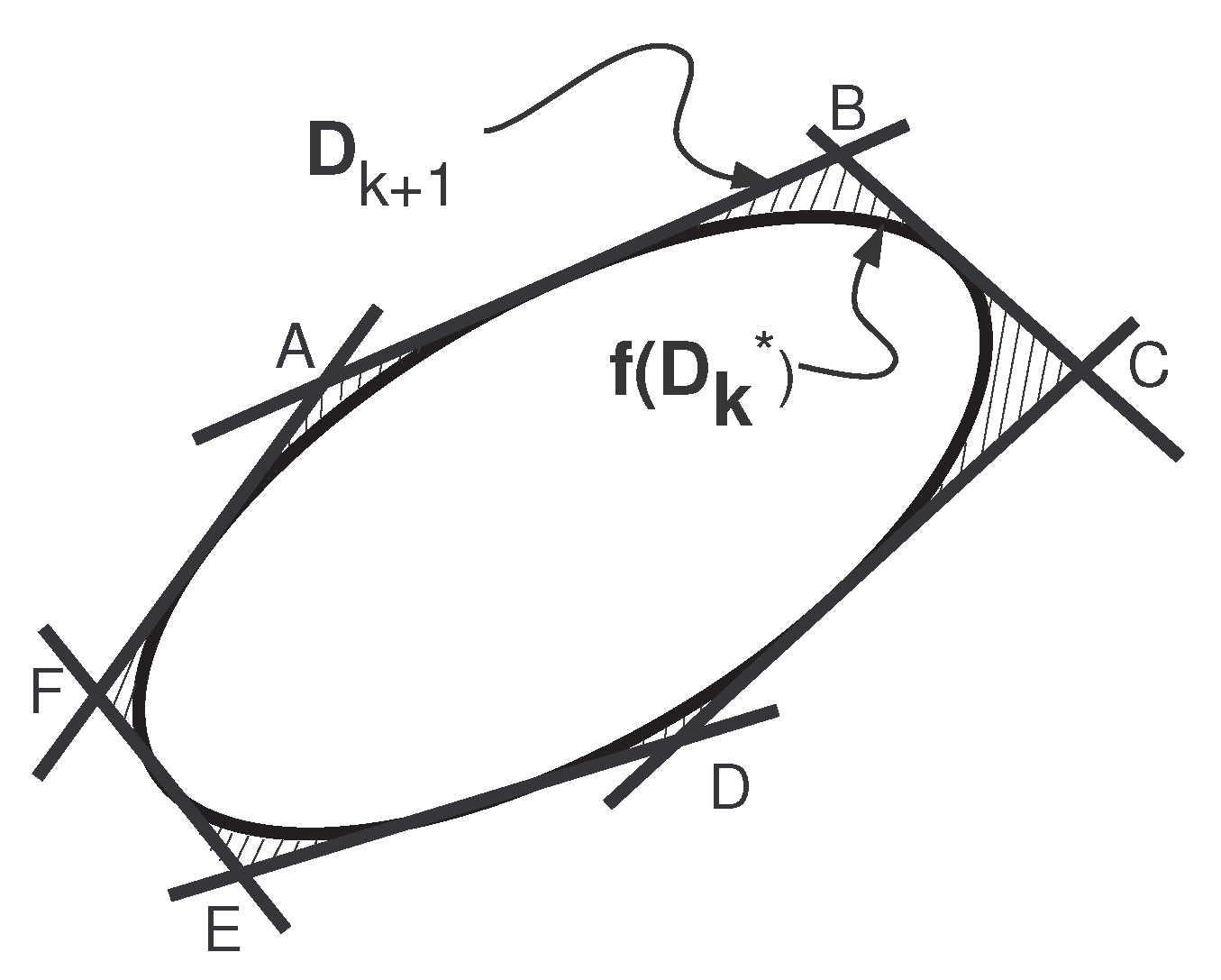
In order to minimize the error, we need to make sure that the true reachable set  D k *  is a subset of estimated reachable sets  D k  so that if  { D k } { 0 }  as  k , it guarantees that  { D k * } { 0 } , which proves that (3) is globally asymptotically stable. An example of using linear boundaries to approximate a convex reachable set is shown in Figure 2. The linear approximation has the advantage that increasing the number of linear functions will increase the accuracy. If the number of linear functions goes to infinity, then  D k + 1 D k + 1 * .
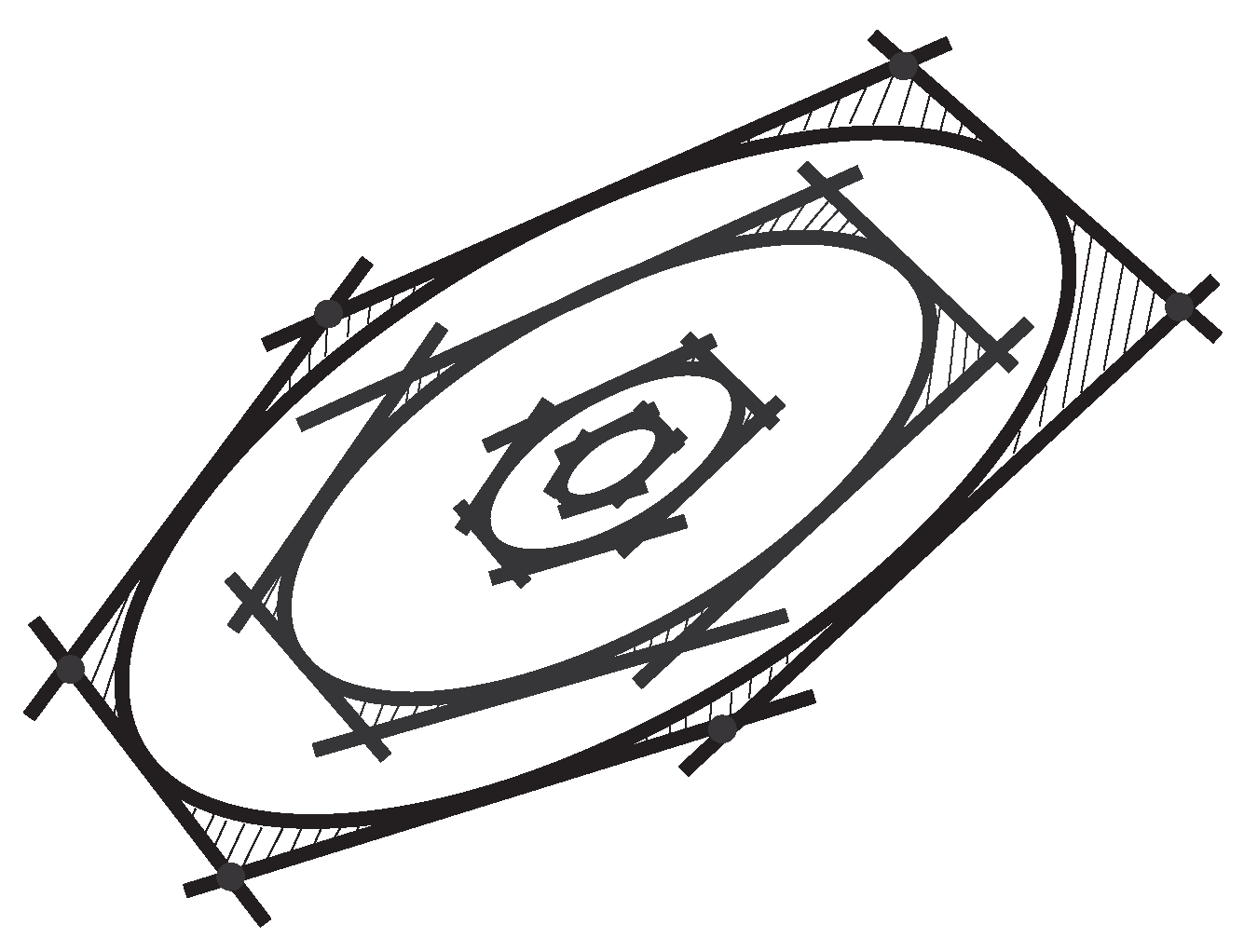
Figure 3 illustrates how the accuracy of the estimation of the convex reachable set can be increased by increasing the number of linear boundaries.
In the next section, a linear approximation of the reachable set is explained. Then, the approximated reachable set is used to detect the stability region for the equilibrium point for system (3).

5. RODD-LB1 [9]

Reduction of Dissipativity Domain is a numerical algorithm to detect the stability of the equilibrium point for a dynamic system. The better the accuracy of the estimated reachable set, the more accurately the algorithm can detect stability or instability. The estimated reachable set at time step  k + 1 ( D k + 1 )  is compared against the estimated reachable set at the previous time step  k ( D k ) . If the size of the estimated set decreases over time, then this is an indication of the asymptotic stability of the equilibrium point.
For RODD-LB methods, reachable sets are approximated with linear boundaries. These boundaries take the form [9]
q i T x γ i
where  q i  is a unit vector that is orthogonal to the boundaries.
The RODD-LB1 method involves three main steps. These steps are given as follows:

5.1. Step 0

Step 0 is the internalization step, where the initial approximate reachable set  D 0  is defined. The unit vectors  q 0 , j  are chosen to be  { e 1 , , e n , e 1 , , e n } , where  e i  is the unit vector along axis i. Then, we compute
γ 0 , j = max x { q 0 , j T f ( x ) : x R n } , j = 1 , 2 , , m 0
where  m 0 = 2 n . The set  D 0  can then be defined:
D 0 = { x : q 0 , j T x γ 0 , j , j = 1 , 2 , , m 0 }

5.2. Step 1

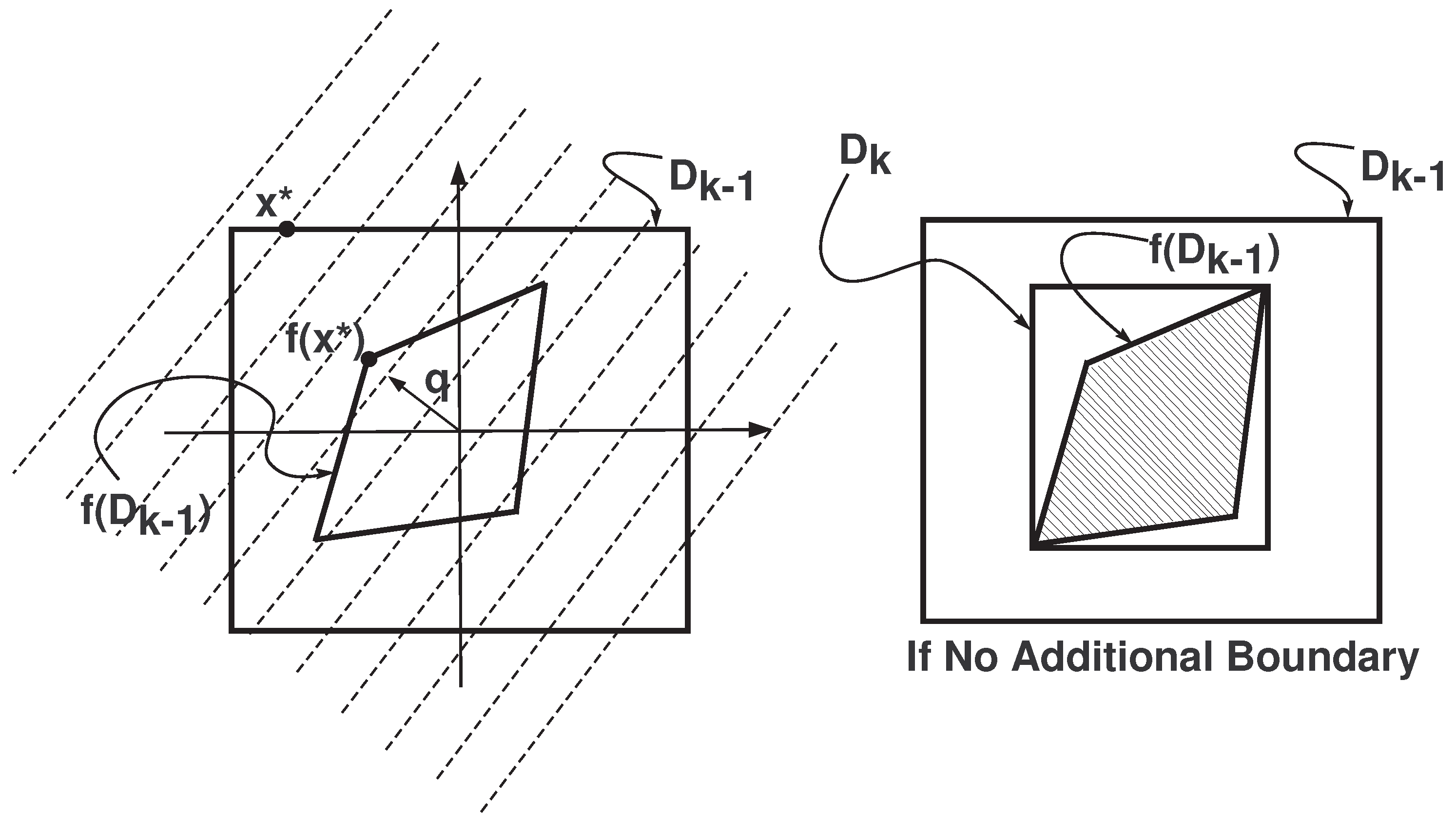
In this step, the size of the set  D k  decreases as k evolves over time. This can include both moving existing boundaries and adding new boundaries. In step 1, the boundaries from the previous iteration are moved (see Figure 4). This involves updating  γ k , j :
γ k , j = max x { q k , j T f ( x ) : x D k 1 }
where  j = 1 , 2 , , m k . According to the Extreme Value Theorem [14], the maximum of the function in (11) is achievable. This is because the estimated reachable set  D k 1  is a compact set, and  q k , j T f ( x )  is a continuous function. Since  γ k , j  is always imputable, the estimated reachable set  D k  can be defined as follows:
D k = { q k , j T x γ k , j , j = 1 , 2 , , m k }
By definition, the estimated reachable set  D k  is the set of linear functions that are tangent to the set  f ( D k 1 )  (see Figure 5). The optimization in (11) guarantees the tangency. The decision to add additional linear boundaries depends on the shrinkage of the estimated reachable set. If it is necessary to add more linear boundaries, then the algorithm switches to step 2. If the set  D k  decreases in size compared to the set  D k 1 , then additional linear boundaries are not required. In this case, an accurate approximation of the true reachable set  D k *  is obtained, and improving the estimation accuracy is not needed. However, if the estimated reachable set  D k  does not decrease in size compared to  D k 1 , then there is a need to improve the accuracy of the estimated reachable set. The accuracy improvement of the estimated reachable set will be realized by including additional linear functions. In this case, the algorithm switches to step 2.

5.3. Step 2

If the estimated reachable set  D k  does not decrease in size compared to the set  D k 1 , then there are two possibilities: Case I: The equilibrium point is not globally asymptotically stable. Case II: The estimated reachable set  D k  is not an inaccurate estimation of the true reachable set  D k * . To reduce the estimation error and make the estimated reachable set more accurate, a new linear function is added.
To minimize the estimation error, there is a need to find an optimal boundary line  q . The calculation of the vector  q  can be performed by solving the double maximization problem that maximizes the following difference [9]:
q T x * max x D k 1 { q T f ( x ) }
where  x *  is the solution that maximizes the function  q T f ( x ) , and  f ( x * )  is located on the boundary of  f ( D k 1 ) . Equation (13) represents the distance that a new boundary would move in one time step, and we want to add the boundary with which we will obtain the maximum shrinkage of  D k . Figure 5 is a typical representation of how  D k  is derived when step 1 is performed. The dashed lines are an indication of the contour lines of  q T x . There are two maximization problems involved in (13). The inner one locates the  x *  that is in the next iteration of (3) and located on the boundary of  D k 1 . The outer maximization in (13) guarantees finding the best direction of the vector  q  that creates the largest distance of this boundary line from  D k 1  to  D k . The new linear boundary will be located on the surface of  f ( D k 1 )  at the point  f ( x * ) . This is the optimal location that corresponds to the largest unwanted region from the estimated reachable set.
The interior maximization in (13) searches for the optimal  x  only over the space of those points coming from the solution of the optimization in (11), not over all possible points in space. This makes the optimization simple, but at the potential cost of missing the new optimal boundary. The maximization problem to find  q  in [9] is written as follows:
q j = a r g max q = 1 { q T x j max x i { q T f ( x i ) } : i = 1 , 2 , , m }
where  x j j = 1 , 2 , , m , denotes the solution of the optimizations in (11). These are the points that are located on the boundary of  f ( D k 2 ) . There are several reasons why limiting the search space to the inner optimization in (14) is impractical. First, for a linear  f ( D k 2 ) , tangent points for the m current boundaries of  D k  always occur at the vertices. Second, even if we were to include all of the vertices,  x j , of  D k  in the inner maximization of (14), there is no guarantee that the points  f ( x j )  will be vertices of  f ( D k ) . Lastly, for the reachable set with nonlinear boundaries, the maximum can occur at any location and not necessarily the vertices. A slight modification of the current method is introduced in the next section that solves the above limitations and speeds up the convergence rate of the algorithm.
After finding  q j  for  j = 1 , 2 , , m  in (14), the RODD-LB1 algorithm selects  q j  with the largest values of
θ j = θ 1 , j θ 2 , j
where
θ 1 , j = max x { q j T x : x D k 1 } θ 2 , j = max x { q j T f ( x ) : x D k 1 }
Once the estimated reachable set has been updated, and  D k  has been obtained (using (11) with the new boundaries included), the algorithm checks again to verify that there has been a sufficient reduction in size from  D k 1  to  D k . If the reachable set with updated linear boundaries does not decrease in size, then the algorithm is inconclusive. In this case, the algorithm stops. If the additional linear boundaries help to reduce the size of the reachable set, then the algorithm continues with step 1. The algorithm stops if the size of the reachable set reaches below some small threshold value. This means that the equilibrium point of the dynamic system is stable.

6. RODD-LB2

RODD-LB1 suffers from a limited search space for finding optimal linear boundaries. In RODD-LB2, this problem is resolved, which generates a better estimation of the reachable set and which we have found to converge faster on several test problems compared to RODD-LB1. RODD-LB2 provides an improvement in the maximization of step 2 compared to RODD-LB1. The objective in RODD-LB2 is to widen the search space, which requires a somewhat larger computational burden at each iteration, but the improved boundaries may allow the algorithm to converge faster. In order to improve the inner optimization of (14), instead of searching for the optimal  x  in the space among the points provided by (11), we add all of the vertices of  D k  to the search space. We found that adding these points makes RODD-LB2 more efficient in higher dimensions.
In RODD-LB2, the derivation of  q j  in (14) is revised based on the discussion in [13] as follows:
q j = a r g max q = 1 { q T x j max x i Ω { q T f ( x i ) } }
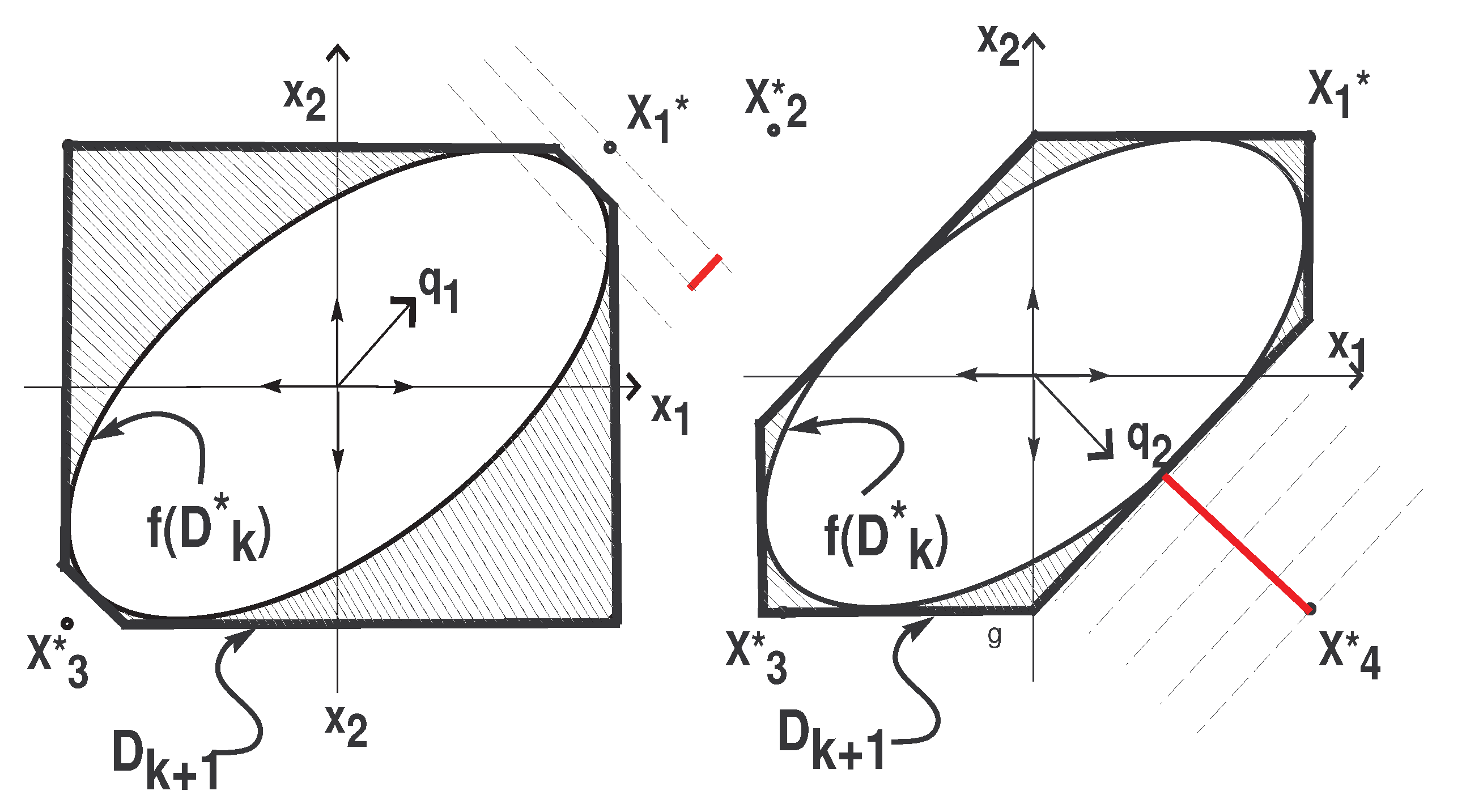
where  Ω  is the space containing all the vertices of the set  D k  and where  x j Ω . The concept of RODD-LB2 is illustrated with the 2D example shown in Figure 6.
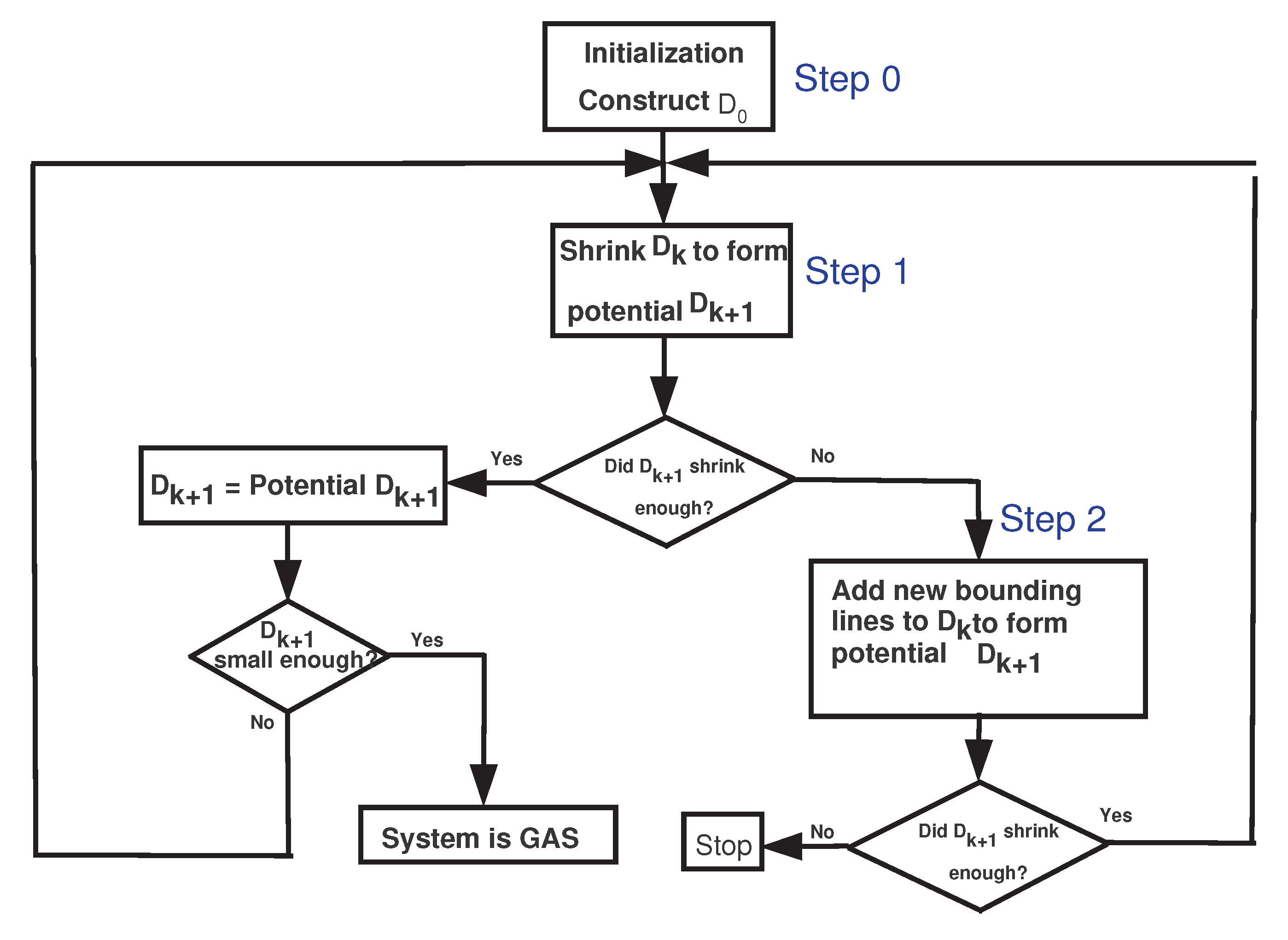
The left graph in Figure 6 used the RODD-LB1 method to estimate the reachable set, whereas the right graph in Figure 6 used the RODD-LB2 method. As shown in the figure, the wider search space in the RODD-LB2 algorithm ends in a better estimation of the true reachable set. All the steps inside the RODD-LB2 algorithm are shown in the flowchart below(see Figure 7).

7. RODD-EB

The RODD-EB method uses elliptical boundaries, instead of linear boundaries, to create the approximate reachable sets. As with the RODD-LB methods, RODD-EB requires that the approximate reachable set  D k + 1  contain the reachable set  D k + 1 * . In RODD-EB, the boundaries are created with quadratic functions, and the approximate reachable sets are ellipses.

7.1. RODD-EB Algorithm

In this section, we explain the implementation of the RODD-EB method. The RODD-EB algorithm can be divided into three steps.

7.1.1. Step 0

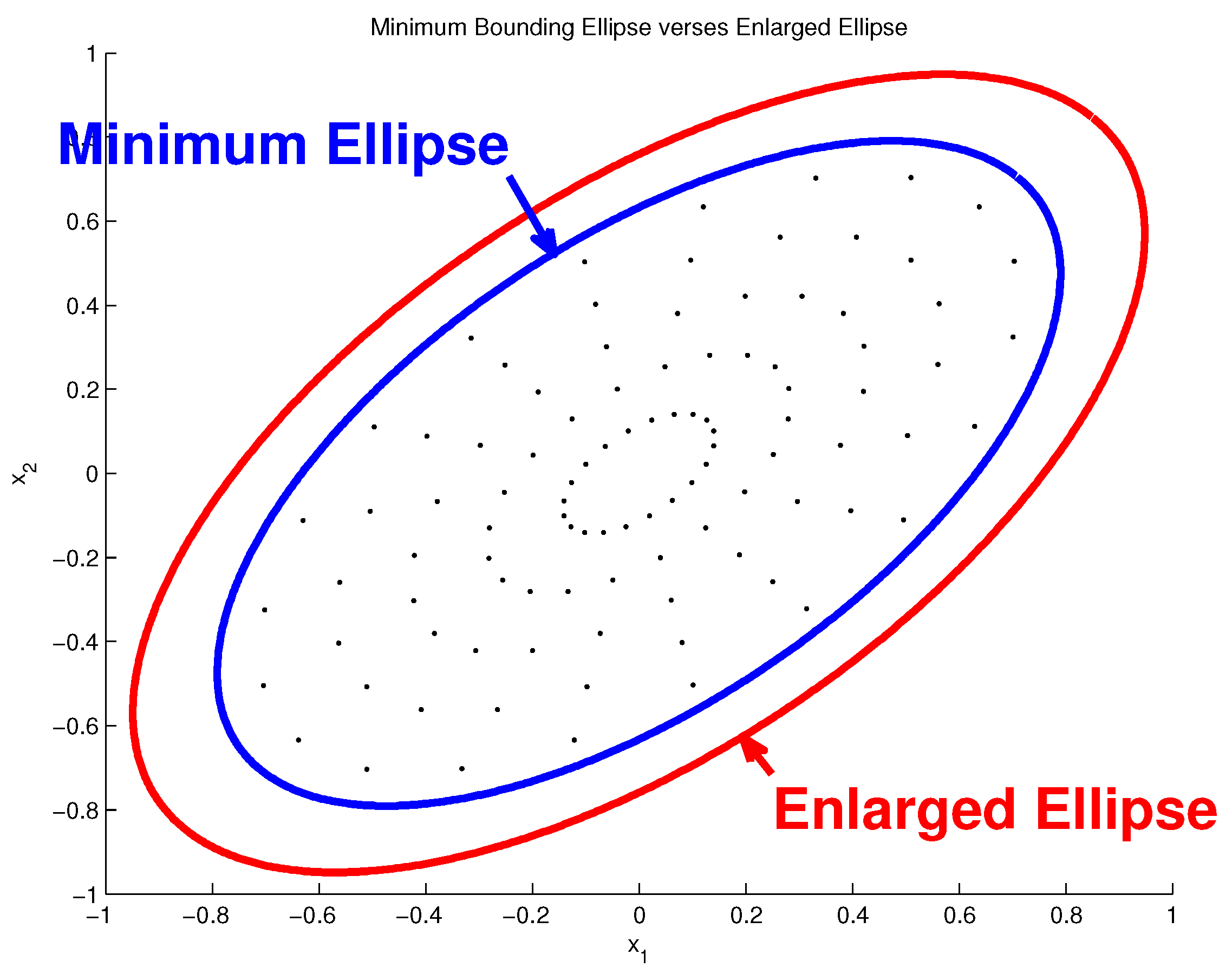
As with the RODD-LB methods, the first step is to find the initial approximate reachable set,  D 0 . This can be carried out numerically in a variety of ways, and the exact technique used is not critical to the success of the algorithm. For our simulation experiments, we randomly generated a large number of points throughout the feasible region of the state space, updated the points at one time step using (3), and then found the minimum volume ellipse that contained all these points. We would then increase the size of the ellipse by  20 %  to account for any errors. Figure 8 illustrates a sample calculation of  D 0 . The elliptical set  D 0  is defined by a positive definite symmetric matrix  E 0 , as in [11]:
D 0 = { x R n | x T E 0 x 1 }

7.1.2. Step 1

In this step, the set  D k + 1  is constructed from the set  D k  by shrinking the size of the ellipse. This is similar to step 1 of the RODD-LB methods. The update involves the following maximization process [13]:
γ k + 1 = max x { f ( x ) T E k f ( x ) : x D k } E k + 1 = E k γ k + 1
where  D k = { x R n : x T E k x 1 } . The maximization in (19) has a solution, and  γ k + 1  is computable, because the set  D k  is compact, and the function  f  is continuous. In order to be consistent with the definition of  D k , we normalize  E k  by  γ k + 1 . Then, if  γ k + 1 < 1 , the set  D k + 1  shrinks compared to  D k . The set  D k + 1  derived in this step is only a potential  D k + 1 , because if  D k + 1  does not decrease compared to  D k , then the orientation of  D k + 1  needs to be changed. In this case, the algorithm switches to step 2.
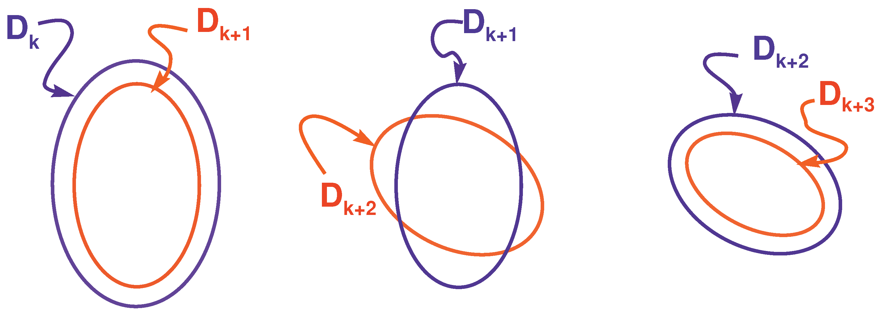
Figure 9 illustrates a typical 2D example of a system with a GAS equilibrium point, for which  D k + 1  shrinks relative to  D k . If the equilibrium point of a system is GAS, and if  D k  ( E k ) is oriented correctly, then  x T E k x 1  is a good estimation of the reachable set. For stable linear systems, there always exists an elliptical reachable set, and for nonlinear systems with a stable equilibrium point, an appropriate elliptical set can often make a good estimation of the reachable set.

7.2. Step 2

If the set  D k + 1  does not decrease in size compared to the set  D k , then either the equilibrium point cannot be shown to be stable using an elliptical  D k , or the orientation of the ellipse  D k  needs to be changed.
There is a close relationship between the selection of an approximate reachable set and the selection of a Lyapunov function. If we select the Lyapunov function  V ( x , E ) = x T E x , then we can define  D k = { x R n | V ( x , E ) 1 } . Consider a point on the boundary of  D k  —  x k b . When this point is updated in time, it moves to  f ( x k b ) . The change in the Lyapunov function would be
V = ( x k b ) T E ( x k b ) f ( x k b ) T E f ( x k b )
In terms of both the choice of the Lyapunov function and the choice of the approximate reachable set, we would like  V  to be as large as possible. For the reachable set, we would like to choose  E  so that  V  is maximized for every  x k D k . However, the  E  that maximizes  V  generally depends on  x k . A conservative (robust) solution would be to chose the  E  that maximizes the minimum  V  over all  x D k . This can be formulated as follows:
max E > 0 { min x D k { x T E x f ( x ) T E f ( x ) } }
If the maximum of the minimum  V  over  x  is positive, then it is guaranteed that the set  D k + 1  contains all the system solutions at time step  k + 1  and has a reasonable orientation. In this case,  D k + 1  is a good estimation for  D k + 1 * , and the algorithm continues with the new  E  in step 1. Figure 10 graphically explains the max–min optimization in (21). The dashed ellipses are contour lines of a potential  V ( x , E ) . For the potential V V > 0  for the point  x 1 , and  V < 0  for the point  x 2 . The contour lines for the optimal V are shown by the solid lines, where, for all  x D k V > 0 . The purpose of (21) is to find an orientation for  D k  so that  f ( D k ) D k . This is equivalent to finding a quadratic Lyapunov function that will decay for all trajectories.
Figure 11 shows the direction field for a stable 2D dynamic system. In this figure, the solid lines represent contour lines for a  V ( x , E )  that does not produce a good estimation of the reachable set, and the dashed ellipses represent a better  V ( x , E ) . The solid ellipses do not produce a good estimation of the reachable set, because  V  is not positive for all  x D k ; by inspecting Figure 11, it can be observed that some trajectories are going out of the solid ellipses. However, the dashed ellipses produce a good estimation of the reachable set, because  V  is positive for all  x D k . (All trajectories are moving inside the dashed ellipses.)
The exact method for finding the optimal ellipse (a more precise formulation of (21)) is given by [11]:
E k = max E { min x { x T E x f ( x ) T E f ( x ) : x T E k 1 x 1 } : min ( e i g ( E ) ) > 0 , max ( e i g ( E ) ) < 1 } γ k = max x { f ( x ) T E f ( x ) : x T E k 1 x 1 } E k = E k γ k
The inner minimization in (22) minimizes  V  over  x D k  for fixed  E , whereas the outer maximization finds the optimal  E  to maximize the minimum value of  V . The inner minimization is constrained by  x T E k 1 x 1 , because  x  needs to be in  D k 1 , and the outer maximization is constrained by  min ( e i g ( E ) ) > 0  and  max ( e i g ( E ) ) < 1 . The minimum eigenvalue of  E  is forced to be positive, because  E  needs to be positive definite, and the maximum eigenvalue of  E  is forced to be less than 1 to bound  E  and to ensure the existence of a maximum. (The magnitude of the largest eigenvalue of  E  does not affect the orientation of  D k ). As in step 1, we always normalize  E k  by  γ k . In order to check whether  D k  has shrunk relative to  D k 1 β k  is defined as follows:
β k = max { | | x x * | | 2 : x D k }
If  β k < β k 1 , then  D k  has shrunk relative to  D k 1 . If  D k  has not decreased enough, then no conclusion can be made about stability. In this scenario, the algorithm is inconclusive and will exit. If a reachable set decreases over time, then there is no need to add additional linear boundaries. The algorithm tests to see whether the size of  D k  is essentially zero to stop and exit.
All the steps inside the RODD-EB algorithm are shown in the flowchart below(see Figure 12).

8. RODD-Hybrid

The RODD-Hybrid method switches between RODD-LB and RODD-EB as the algorithm progresses. The RODD-LB methods approximate reachable sets with a set of linear boundaries. These methods are guaranteed to detect stability if a sufficient number of linear boundaries are used. The main drawback of these methods is the slow rate of convergence, because they may require many linear boundaries to adequately approximate the reachable set. Alternatively, the RODD-EB method is an algorithm with a fast rate of convergence if the reachable set is approximately quadratic. This is generally true near the equilibrium point, but it may not be true in the early iterations of the algorithm. The flexibility of linear boundaries might be useful at certain stages of the algorithm, while the efficiency of elliptical boundaries could provide better performance at other stages. The need for an accurate and fast algorithm for proving the global asymptotic stability of dynamical systems led us to develop a new algorithm based on a combination of RODD-LB2 and RODD-EB. RODD-Hybrid combines RODD-LB2 and RODD-EB by switching between them at various iterations of the algorithm.
The main goal in the RODD-Hybrid method is to obtain an accurate approximation of reachable sets with the fastest rate of convergence. In order to accomplish this goal, the RODD-Hybrid algorithm is divided into three main modes, RODD-LB2, RODD-EB and transition modes. The RODD-Hybrid method can start with either RODD-LB2 or RODD-EB.

8.1. RODD-EB Mode

Suppose that the RODD-Hybrid method starts with RODD-EB. In this case, the RODD-Hybrid algorithm uses (19) to derive  D k + 1 . If  D k + 1  does not decrease compared to  D k , then the algorithm uses (22) to find a better estimation of the reachable set. Unlike the RODD-EB algorithm, the RODD-Hybrid algorithm only allows one re-orientation of  D k . If the re-oriented  D k  does not make  D k + 1  shrink compared to  D k , then the algorithm switches to RODD-LB2. The transition from RODD-EB to RODD-LB2 will be explained in the transition mode section.
Figure 13 graphically illustrates the RODD-EB mode of the RODD-Hybrid algorithm. If the set  D k + 4  does not decrease compared to  D k + 5 , then the algorithm switches to the RODD-LB2 mode.

8.2. Transition from RODD-EB to RODD-LB Mode

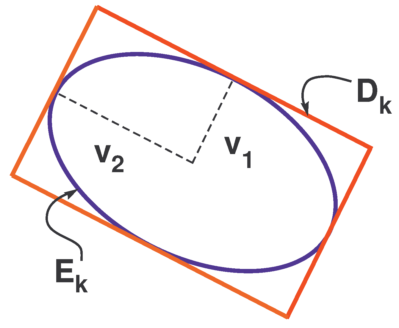
The RODD-LB2 mode of RODD-Hybrid will take over when one re-orientation of the set  D k  does not make  D k + 1  shrink compared to  D k . When RODD-Hybrid needs to switch from the RODD-EB mode to the RODD-LB mode,  D k  needs to be converted from an ellipse to a polytope. To produce the polytope with the lowest volume, we use the eigenvectors of  E k , as shown in Figure 14. The bounds of the optimal bounding polytope are derived through the following optimization [11] (similar to (11)):
γ k , i = max { v i T x : x T E k x < 1 }
where  { v 1 , v 2 , v n }  are the eigenvectors of  E k . The sides of the bounding polytope are orthogonal to the eigenvectors  v i , and the optimization in (24) derives the bound such that the sides are tangent to the original elliptical  D k . From this point, the reachable set will be approximated by the bounding polytope  D k . Figure 14 shows the bounding polygon ( n = 2 ) derived through the optimization given in (24).

8.3. RODD-LB2 Mode

In the RODD-LB mode,  D k + 1  is updated through (11) and (12). If the reachable set  D k + 1  decreases in size compared to the set  D k , then there is no need to add additional linear boundaries. However, if  D k + 1  does not decrease relative to  D k , then additional linear boundaries are added. The additional linear boundaries are calculated through the optimization given in (14). If the additional linear boundaries do not make  D k + 1  shrink relative to  D k , then the algorithm is inconclusive and will stop. Otherwise, the algorithm will continue until the number of additional linear boundaries exceeds the maximum allowable number. Based on many experiments, we found that  4 n  is a reasonable upper bound for the maximum number of linear boundaries. If  D k  does not decrease enough, and the algorithm exceeds the maximum number of linear boundaries, then the algorithm will switch to the RODD-EB mode. The transition from RODD-LB2 to RODD-EB is explained in the next section.
Figure 15 graphically illustrates the RODD-LB2 mode of the RODD-Hybrid algorithm. If the set does not shrink compared to  D k + 1 , then the algorithm will switch to the RODD-EB mode using the bounding ellipse  E k + 1 .

8.4. Transition from RODD-LB to RODD-EB Mode

In the transition between the RODD-LB mode and the RODD-EB mode, a bounding ellipse is calculated to enclose the final set  D k  from the RODD-LB2 mode. The first step is to find a set of points on the boundary of  D k . These points will be the vertices of the linear boundaries and certain locations in the middle of the boundaries. Each linear boundary is defined by a unit vector  q i  that is orthogonal to the boundary. In other words, the  i t h  boundary is defined as those points  x  such that
q i T x = γ i
The point  x = γ i q i  is on the  i t h  linear boundary, because it satisfies (25). Some of these points may not fall on the edge of  D k , because the set  D k  in RODD-LB2 may be the interior of several linear boundaries. The set  D k  is defined as follows:
D k = { x R n | q i T x γ i : i = 1 , 2 , , m }
In order to obtain a point on the edge of  D k , we take the inner product of each  q i  with all  q j , including  q i , and divide by  γ j . Then, we find the maximum of  q j T q i γ j . Suppose that the maximum occurs for  q l . Then,  γ l q i q l T q i  is a point on the edge of  D k .
The next step is to find the vertices of  D k . (This can be achieved using the method described in [15].) Then, we form the matrix  Z  as follows:
Z = [ V , M ]
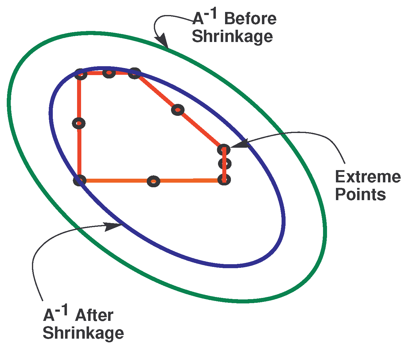
where  V  contains all the vertices, and  M  contains all previously described points on the edges of  D k . Then, we construct the approximate covariance matrix  A = Z Z T . Using concepts from principal component analysis [16], the expression  x T A 1 x = γ  gives a reasonably good orientation of the bounding ellipse. The correct value for  γ  can be found from the optimization in (19), where the constraint is the final  D k  in the RODD-LB2 mode. After  γ  is found, the set  D k + 1  is derived from  D k  using RODD-EB. Figure 16 illustrates the transition mode from RODD-LB2 to RODD-EB for a specific 2D example.
In the following section, some examples are used to compare the efficiency of the proposed algorithms.

9. Discussion

9.1. Examples

Example 1.
Consider a two-layer RNN with 10 neurons in the hidden layer:
x ( k + 1 ) = B tanh ( W x ( k ) + b )
where  x R 2 B R 2 × R 10 W R 10 × R 2  and  b R 10 . For a specified set of weights, this system has the GAS equilibrium point  z = [ 0.8248 , 0.7799 ] T . (For all figures, we move this to the origin.) All the RODD methods were able to detect stability; however, RODD-LB2 has the fastest speed of convergence. This is due to the shape of the reachable set. The left figure in Figure 17 shows the randomly generated points used to create  D 0 . The middle figure in Figure 17 shows  f ( D 0 )  and the linear boundaries of  D 1  for RODD-LB2, and the right figure in Figure 17 shows the elliptical bounding of  D 1  for RODD-EB.
In this case, linear boundaries can approximate the reachable set better than elliptical boundaries. Hence, RODD-LB2 has the fastest speed of convergence (4x faster). Although RODD-EB could detect the GAS equilibrium point, due to the shape of the reachable sets, this method is not as fast as RODD-LB2. RODD-Hybrid does not have the fastest speed of convergence for this example, because it starts in RODD-EB mode, and that affects the overall speed of convergence.
The graphs of  β k  for RODD-LB2, RODD-EB and RODD-Hybrid are shown in Figure 18. Note that for RODD-EB, the graph of  β k  is not always decreasing. This is because of the change in the orientation of  D k .
Example 2.
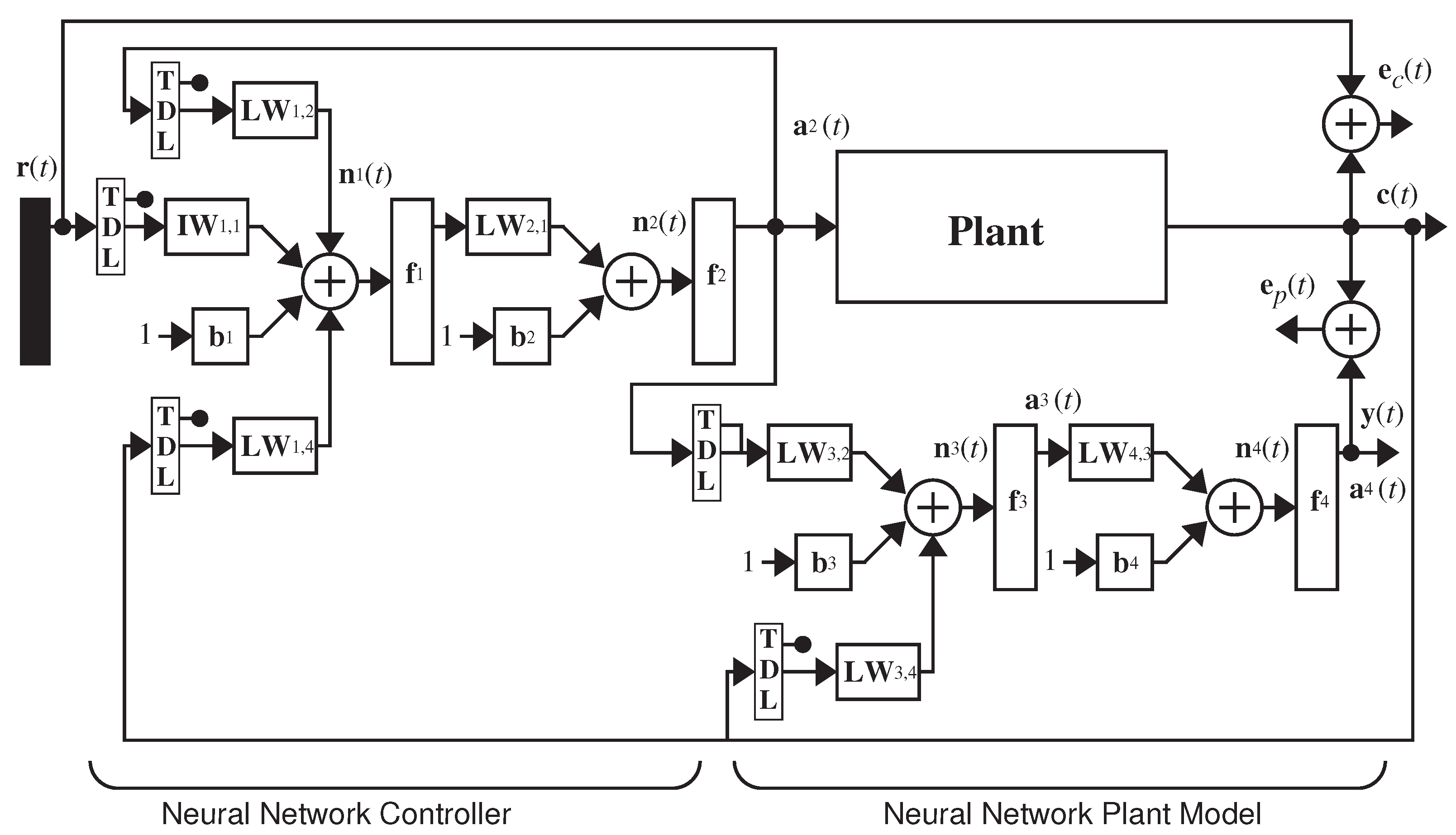
The second example is the model reference control of a single-link robot arm. The system model and the controller were trained using the Neural Network Toolbox of MATLAB [17] using the procedure described in [11]. The system block diagram is shown in Figure 19. This is a special case of an LDNN network, as defined in Equation (1). The proposed stability methods can now be applied to the state equation. Figure 20 shows the graphs of  β k  for RODD-LB2 and RODD-EB and Hybrid. All the RODD methods were able to detect the stability of the equilibrium point for this example. In this example, RODD-EB and Hybrid have the same graph for  β k . This is because RODD-Hybrid starts with the RODD-EB method, and, in this example, RODD-Hybrid never goes to the RODD-LB2 mode.
Table 1 illustrates the result of stability for different methods. RODD-EB(RODD-Hybrid) is more efficient in detecting the stability of the equilibrium point compared to RODD-LB2. In this example, RODD-EB (RODD-Hybrid) is 1.07 times faster than RODD-LB2.

9.2. Comparing Performance

The performance of the proposed algorithms was tested using several random RNN systems. A total of 60 randomly generated RNN systems were used to compare the performance of RODD-LB2, RODD-EB and RODD-Hybrid versus the original method, RODD-LB1. The final results show an improvement (average speed of convergence) in all proposed algorithms compared to RODD-LB1. The improvement results are given in Table 2.

10. Conclusions

In this paper, we propose three stability analysis algorithms that use the method known as Reduction of Dissipativity Domain [9,13]. The objective of the proposed algorithms is to find whether the origin is globally asymptotically stable. The proposed algorithms work by checking the size of the reachable set as the system evolves over time and illustrating that the evolved reachable set finally converges to the origin. RODD-LB1 and RODD-LB2 use linear approximations of the reachable set, and RODD-EB uses quadratic approximations. The RODD-Hybrid algorithm, which combines linear and quadratic approximations of reachable sets, takes the advantage of the accuracy of RODD-LB and the fast convergence of RODD-EB. Preliminary tests on a variety of systems have shown that RODD-Hybrid is more efficient than RODD-LB1, RODD-LB2 or RODD-EB.
The proposed methods open up many interesting theoretical and practical research possibilities. The methods that we developed in this study can be applied to solve interesting problems, i.e., maintaining stability during RNN training or approximating the region of attraction [11]. One of the main challenges with RNNs is training. The potential instability of RNNs complicates their training. The spurious valleys in the training error surface that were studied in [3] are an immediate consequence of the potential instability. However, the new efficient stability algorithms open up the possibility of maintaining stability during RNN training. This will guarantee the smoothness of the error surface and improve training performance.
One of the great features of the RODD methods is the fact that the initial set can be selected arbitrarily. Moreover, this set can be placed at any desired location. In this research work, we were looking for GAS equilibrium points. However, RODD methods can be applied to nonlinear systems with multiple stable equilibrium points. In this case, each stable equilibrium point has a region of attraction. By changing the size and location, we could use RODD methods to approximate the region of attraction of selected equilibrium points.

Funding

This research received no external funding.

Data Availability Statement

Not applicable.

Conflicts of Interest

The authors declare no conflict of interest.

References

  1. Hu, S.; Liu, Y.; Liu, Z.; Chen, T.; Wang, J.; Yu, Q.; Deng, L.; Yin, Y.; Hosaka, S. Associative memory realized by a reconfigurable memristive Hopfield neural network. Nat. Commun. 2015, 6, 7522. [Google Scholar] [CrossRef] [PubMed] [Green Version]
  2. Lin, H.; Wang, C.; Cui, L.; Sun, Y.; Zhang, X.; Yao, W. Hyperchaotic memristive ring neural network and application in medical image encryption. Nonlinear Dyn. 2022, 110, 841–855. [Google Scholar] [CrossRef]
  3. Horn, J.; De Jesus, O.; Hagan, M.T. Spurious Valleys in the Error Surface of Recurrent Networks—Analysis and Avoidance. IEEE Trans. Neural Netw. 2009, 20, 686–700. [Google Scholar] [CrossRef] [PubMed]
  4. Suykens, J.A.K.; De Moor, B.L.; Vandewalle, J. Nlq theory: A Neural Control Framework with Global Asymptotic Stability Criteria. Neural Netw. 1997, 10, 615–637. [Google Scholar] [CrossRef] [PubMed]
  5. Phan, M.; Hagan, M. Error surface of recurrent neural networks. IEEE Trans. Neural Networks Learn. Syst. 2013, 24, 1709–1721. [Google Scholar] [CrossRef] [PubMed]
  6. Suykens, J.A.K.; De Moor, B.L.; Vandewalle, J. Artificial Neural Networks for the Modeling and Control of Nonlinear Systems; Kluwer: Boston, MA, USA, 1996. [Google Scholar]
  7. Tanaka, K. An Approach to Stability Criteria of Neural-Network Control Systems. IEEE Trans. Neural Netw. 1996, 7, 629–642. [Google Scholar] [CrossRef] [PubMed]
  8. Barabanov, N.E.; Prokhorov, D.V. Stability Analysis of Discrete-Time Recurrent Neural Networks. IEEE Trans. Neural Netw. 2002, 13, 292–303. [Google Scholar] [CrossRef] [PubMed] [Green Version]
  9. Barabanov, N.E.; Prokhorov, D.V. A New Method for Stability of Nonlinear Discrete-Time Systems. IEEE Trans. Autom. Control 2003, 48, 2250–2255. [Google Scholar] [CrossRef]
  10. DeJesus, O.; Hagan, M. Backpropagation algorithms for a broad class of dynamic networks. IEEE Trans. Neural Netw. 2007, 18, 14–27. [Google Scholar]
  11. Jafari, R. Stability Analysis of Recurrent Neural-Based Controllers. Ph.D. Dissertation, Oklahoma State Unioversity, Stillwater, OK, USA, 2012. [Google Scholar]
  12. Khalil, H.K. Nonlinear Systems; Prentice Hall: Hoboken, NJ, USA, 2001. [Google Scholar]
  13. Jafari, R.; Hagan, M. Global stability analysis using the method of reduction of dissipativity domain. In Proceedings of the 2011 International Joint Conference on Neural Networks, San Jose, CA, USA, 31 July–5 August 2011; pp. 2550–2556. [Google Scholar]
  14. Buck, R.; Buck, E. Advanced Calculus, 3rd ed.; McGraw-Hill: New York, NY, USA, 1978. [Google Scholar]
  15. Kleder, M. Constraints to Vertices; Delta Epsilon Technologies, LLC: Mc Lean, VA, USA, 2003. [Google Scholar]
  16. Jolliffe, I.T. Principal Component Analysis, 2nd ed.; Springer: New York, NY, USA, 2002. [Google Scholar]
  17. The MathWorks Inc. MATLAB, Version 7.10.0 (R2010a); The MathWorks Inc.: Natick, MA, USA, 2010. [Google Scholar]
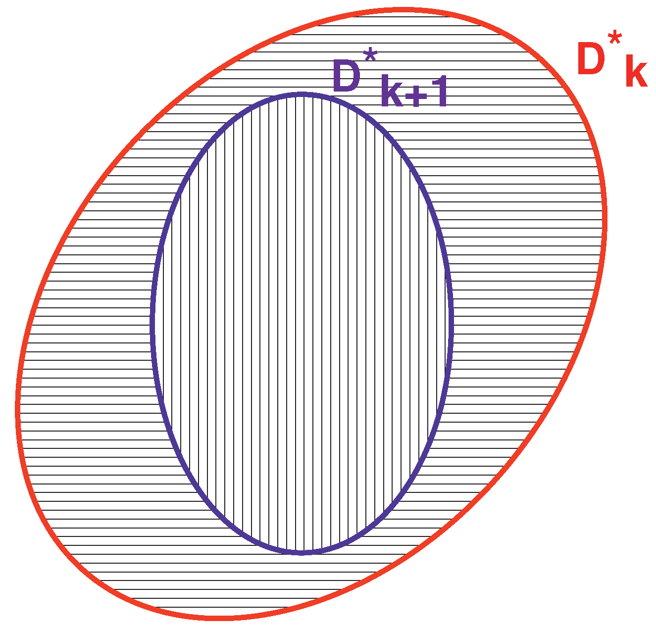
Figure 1. Reachable sets [11].
Mathematics 11 03050 g001
Figure 2. Approximate reachable set [13].
Mathematics 11 03050 g002
Figure 3. More accurate estimation of the reachable set [13].
Mathematics 11 03050 g003
Figure 4. Typical example of RODD-LB1 step 1 [13].
Mathematics 11 03050 g004
Figure 5. Additional linear boundaries [13].
Mathematics 11 03050 g005
Figure 6. Operation of step 2 for RODD-LB1 (left) and RODD-LB2 (right) [13].
Mathematics 11 03050 g006
Figure 7. RODD-LB2 algorithm [13].
Mathematics 11 03050 g007
Figure 8. Minimum bounded and enlarged ellipse [11].
Mathematics 11 03050 g008
Figure 9. Typical example of system trajectory in step 1 [11].
Mathematics 11 03050 g009
Figure 10. Optimal orientation of E [11].
Mathematics 11 03050 g010
Figure 11. Optimal V versus potential V [13].
Mathematics 11 03050 g011
Figure 12. RODD-EB algorithm [11].
Mathematics 11 03050 g012
Figure 13. RODD-EB mode of RODD-Hybrid algorithm.
Mathematics 11 03050 g013
Figure 14. Bounding polygon [13].
Mathematics 11 03050 g014
Figure 15. RODD-LB2 mode of RODD-Hybrid algorithm [11].
Mathematics 11 03050 g015
Figure 16. RODD-LB2 to RODD-EB transition mode [11].
Mathematics 11 03050 g016
Figure 17. Linear boundary  D 1  with RODD-LB2 and RODD-EB.
Mathematics 11 03050 g017
Figure 18. Graph of  β k  for RODD-LB2, RODD-EB and RODD-Hybrid algorithms.
Mathematics 11 03050 g018
Figure 19. Neural network model of MRAC [17].
Mathematics 11 03050 g019
Figure 20. Graph of  β k  for RODD-LB2 and RODD-EB and RODD-Hybrid algorithms, Example 2.
Mathematics 11 03050 g020
Table 1. Comparison of RODD methods—Example 2.
RODD-LB2RODD-EBRODD-Hybrid
ResultStability detectedStability detectedStability detected
Runtime (s)302282282
Improvement1.07xBaseBase
Table 2. Average speed of convergence.
RODD-LB1RODD-LB2RODD-EBRODD-Hybrid
StablebaseImproves by 16xImproves by 75xImproves by 95x
UnstablebaseImproves by 16xImproves by 190xImproves by 112x
Disclaimer/Publisher’s Note: The statements, opinions and data contained in all publications are solely those of the individual author(s) and contributor(s) and not of MDPI and/or the editor(s). MDPI and/or the editor(s) disclaim responsibility for any injury to people or property resulting from any ideas, methods, instructions or products referred to in the content.