Spatial–Temporal Dynamic Graph Differential Equation Network for Traffic Flow Forecasting

Abstract

Traffic flow forecasting is the foundation of intelligent transportation systems. Accurate traffic forecasting is crucial for intelligent traffic management and urban development. However, achieving highly accurate traffic flow prediction is challenging due to road networks’ complex dynamic spatial and temporal dependencies. Previous work using predefined static adjacency matrices in graph convolutional networks needs to be revised to reflect the dynamic spatial dependencies in the traffic system. In addition, most current methods ignore the hidden dynamic spatial–temporal correlations between road network nodes as they evolve. We propose a spatial–temporal dynamic graph differential equation network (ST-DGDE) for traffic prediction to address the above problems. First, the model captures the dynamic changes between spatial nodes over time through a dynamic graph learning network. Then, dynamic graph differential equations (DGDE) are used to learn the spatial–temporal dynamic relationships in the global space that change continuously over time. Finally, static adjacency matrices are constructed by static node embedding. The generated dynamic and predefined static graphs are fused and input into a gated temporal causal convolutional network to jointly capture the fixed long-term spatial association patterns and achieve a global receiver domain that facilitates long-term prediction. Experiments of our model on two natural traffic flow datasets show that ST-DGDE outperforms other baselines.

1. Introduction

Urban transportation systems face significant challenges with rapidly developing urbanization and population growth. Traffic flow prediction, as one of the essential components of intelligent transportation systems (ITS) [1], aims to predict the future state of urban transportation systems (e.g., traffic flow, speed, and passenger demand). As an essential foundation of intelligent transportation systems (ITS), traffic flow prediction has attracted significant attention in deep learning research [2]. Accurate traffic flow prediction is essential and valuable for optimizing traffic management [3], reducing traffic congestion, reducing vehicle emissions, improving traffic safety, improving the urban environment, and promoting economic development [4].

Traffic flow between interconnected roads is closely related due to the complex dynamic connectivity of the traffic road network in the spatial dimension [5]. For example, as time evolves, traffic congestion usually propagates from one road node to its neighboring streets and even to more distant connected road segments [6]. Thus, it is shown that changes in observations generated at a roadway observation point are often related not only to the past historical data of its observation point but also to the past historical traffic data of its neighboring observation points [7,8]. However, most current spatial modeling approaches assume that the spatial correlation is constant, which may not hold in traffic practice.

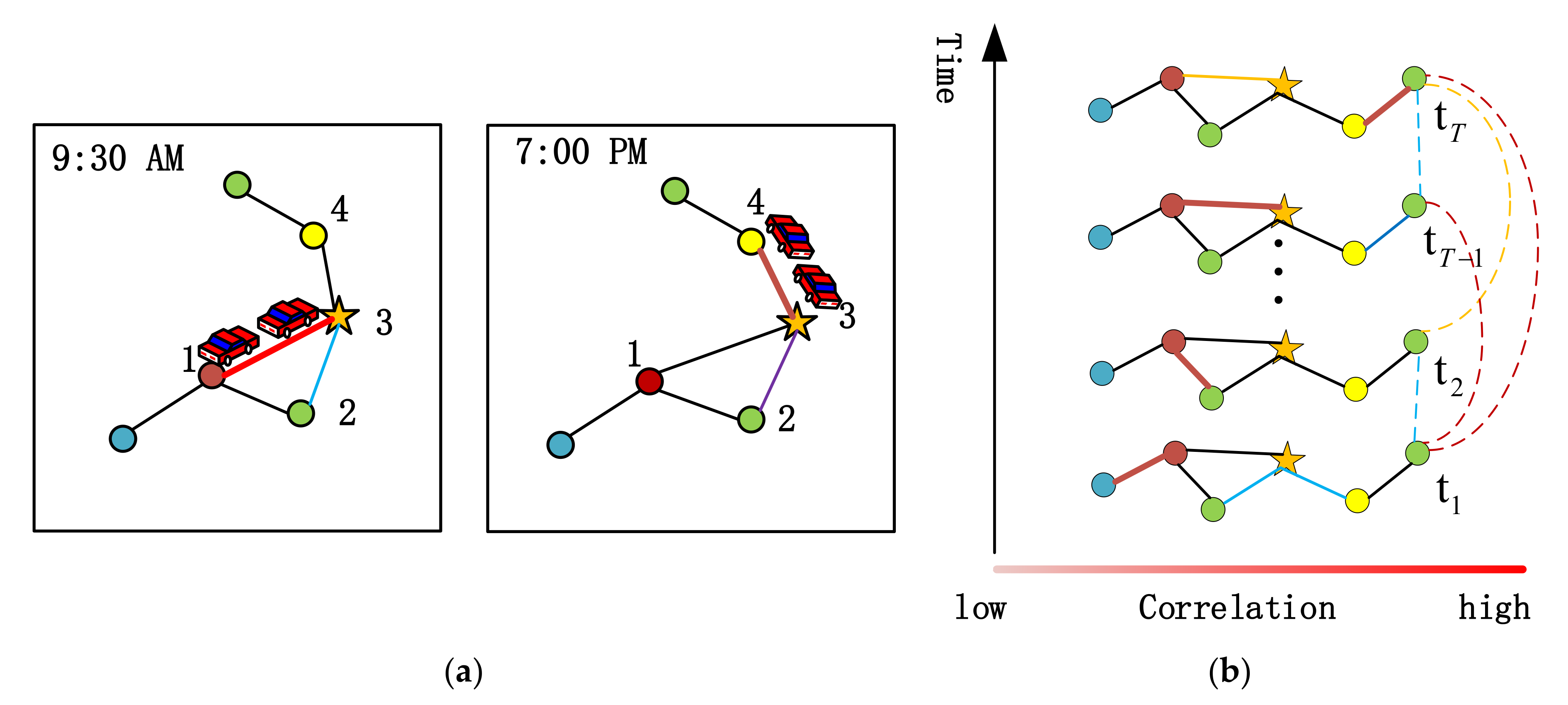
Traffic flows at the observed nodes in each road network show highly dynamic and complex patterns of spatial–temporal correlation [9]. In addition, the degree of relationship between the observation nodes changes dynamically throughout the day as time changes [6]. As shown in Figure 1a, at 9:30 AM, more traffic is observed between node 1 and node 3, indicating a strong correlation between the two points. However, as time changes, there is a substantial correlation between observation node 3 and node 4 at 7:00 PM, and the correlation between nodes 1 and 3 decreases. In addition, the observed values at the exact location at different moments show nonlinear variations, and the traffic state at far time steps sometimes significantly impacts the observed time points more than at similar time steps. As shown in Figure 1b, the correlation degree between the observed values at moment $t_1$ and moment $t_{T-1}$ is more significant than between moment $t_1$ and moment $t_2$. Therefore, it shows that the traffic data has spatial–temporal dynamics and keeps changing with time and space. In addition, the degree of influence of different locations on the predicted position changes dynamically with time [10].

A static adjacency matrix cannot reflect complex and hierarchical urban traffic flow characteristics [11]. For example, in graph convolutional neural network (GCN)-based prediction models [12], the spatial architecture of the road network is represented as a predefined adjacency matrix. However, in real applications, the traffic signal over a while can be decomposed into a smooth component determined by the road topology (connectivity and distance of sensors at observation points) and a dynamic component determined by the real-time traffic state and unexpected events. 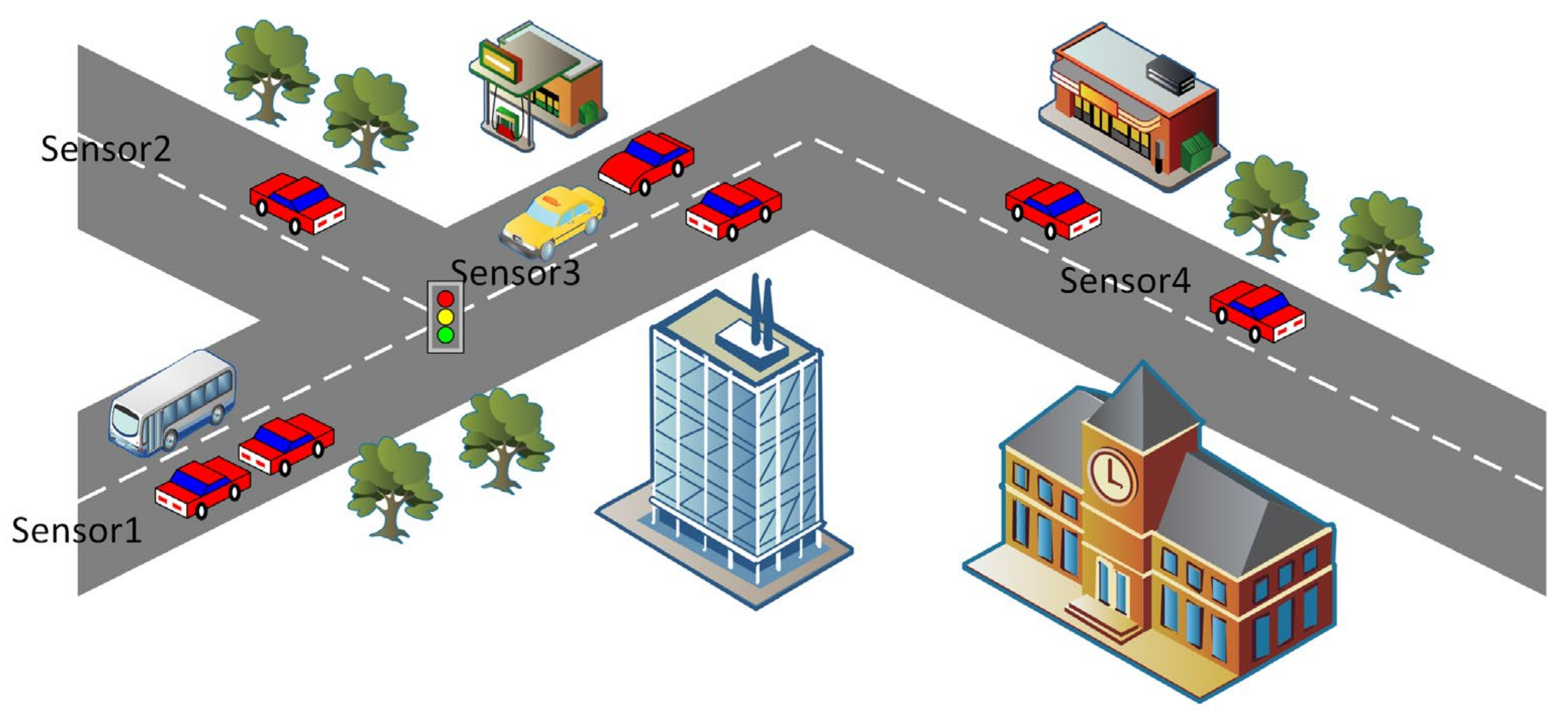As shown in Figure 2 the traffic flow is cross-regional, and a change in traffic flow in one region inevitably leads to a change in another region. Traffic flow in the Sensor 1 region changes over time, gradually flowing to the Sensor 3 region over a more extended period, possibly to the Sensor 2 region. Therefore, the hidden dynamic spatial–temporal relationship between regions must be considered simultaneously when spatial–temporal modeling. Considering the complex dynamical characteristics of urban traffic flow, existing GNN methods use predefined adjacency matrices to learn the spatial correlations between different observed nodes, which inevitably limits the model to learning the spatial–temporal characteristics of urban traffic dynamics. However, most current works must integrate them while maintaining efficiency and avoiding over-smoothing.

Due to the powerful ability of graph neural networks to capture spatial correlation from non-Euclidean traffic flow data [13], they can effectively characterize geospatial correlation features. With the rapid development of deep learning research, graph neural networks (GNNs) have become the frontier of deep learning research [4] and a popular method in traffic flow prediction tasks, for example, such as STGCN [14], STSGCN [15], LSGCN [16], etc. However, these methods cannot effectively capture the dynamic spatial correlation in the traffic system. Existing GNN-based methods [17,18,19] are usually built on static adjacency matrices (either predefined or self-learning) to learn the spatial correlation between different sensors, even though the influence of two sensors can change dynamically. Although Guo [20] uses self-attention to dynamically compute the correlation of all sensor pairs, its ability to be applied to large-scale graphs is also limited by the complexity of the secondary computation.

Most current research adopts a composition based on predefined static graphs, which fails to consider the dynamic characteristics of traffic flow data. Since traffic data exhibit dynamic solid correlations in the spatio-temporal dimension, mining nonlinear and complex spatio-temporal relationships is an important research topic. On the one hand, methods using static adjacency matrices in graph convolutional networks need to be revised to reflect dynamic spatial correlations in traffic systems. On the other hand, most current methods ignore the hidden dynamic correlations between road network nodes evolving.

Therefore, to solve the above problems, we propose a new traffic prediction framework, the spatio-temporal dynamic graph differential equation network (ST-DGDE). Static distance-based and dynamic attribute-based graphs describe the topology of traffic networks from different perspectives and integrating them can provide a broader view for models to capture spatial dependencies [9]. In conclusion, the contributions of this paper are as follows:

• We extract dynamic features in node attributes using dynamic filters generated by the dynamic graph learning layer at each time step and fuse the dynamic graph generated by node embedding filtering with the predefined static graph. The dynamic graph learning layer is then employed to capture the dynamic graph topology of spatial nodes as they change over time.
• To effectively capture the dynamic spatio-temporal correlations in traffic road networks, this paper uses neural graph differential equations (NGDEs) to learn the hidden dynamic spatio-temporal correlations in spatial and temporal dimensions. Finally, a temporal causal convolutional network and neural graph differential equations are used to successfully model the multivariate dynamic time series in the potential space by intersecting. It is shown through extensive experiments on real road traffic datasets that our proposed algorithm has improved performance compared to several baselines, including state-of-the-art algorithms.

The rest of the paper is organized as follows. We provide a comprehensive overview of the work related to traffic forecasting in Section 2. Section 3 elaborates on the problem definition of traffic forecasting and indicates the study’s objectives. The general framework of our ST-DGDE and the specific solutions are detailed in Section 4. In Section 5, we design several experiments to evaluate our model. Our work and directions for future research are summarized in Section 6.

2. Related Work

2.1. Traffic Flow Prediction

Traffic flow prediction is a typical spatial–temporal sequence prediction problem, and researchers in various aspects have studied traffic flow prediction in the past decades. Regarding research history, traffic flow forecasting methods can be divided into three categories: classical statistical methods models, traditional machine learning models, and deep learning-based models [2]. Classical statistical method models, such as ARIMA [21] and VAR [22], do not capture the dynamic and nonlinear features in traffic flow well in the face of unexpected events in the traffic system. Compared with classical statistical methods models, machine learning methods KNN [23] and SVR [24] can achieve higher prediction accuracy and complex data modeling. Due to the nonlinear characteristics of traffic flow data, machine learning methods have a heavy dependence on feature engineering leading to difficulties in achieving better prediction results. In recent years, deep learning methods can select spatial–temporal data from a high-dimensional perspective for traffic flow prediction. Therefore, some deep learning-based forecasting methods divide the urban area into a spatial raster structure. For example, Ma et al. [25] converted traffic flow data into images using a two-dimensional spatial–temporal matrix for high-accuracy learning and predicting traffic speed. Guo [19] proposed the ST-3Dnet method based on traffic raster data prediction, which introduced 3D convolution to automatically capture the correlation of traffic data in spatial and temporal dimensions. Due to the powerful ability of graph neural networks to capture spatial features from non-Euclidean data [13], many researchers have applied graph convolutional neural networks (GCNs) to capture complex spatial topologies. For example, STGCN [14] integrated a spatial–temporal convolution unit by integrating graph convolutional networks and gated temporal convolution to develop models for spatial–temporal correlations. STSGCN [15] proposed a new graph convolution module to synchronize local spatial–temporal correlation, ignoring the spatial dependencies between cross-regions. Zhao [18] proposed a temporal graph convolution network (T-GCN) to capture the topology of road networks that performs spatial correlation modeling. Most of the above methods mainly learn the spatial dependencies between adjacent regions, thus ignoring the global semantic relationships between regions, resulting in poorly captured long-range spatial dependencies.

2.2. Spatial–Temporal Graph Convolutional Network

Various deep-learning methods have recently been proposed to capture spatial–temporal correlations for traffic prediction. DCRNN [26] proposed a method to model directed traffic flows in the form of diffusion, using codec architectures and scheduled sampling techniques to improve long-term prediction performance. Zhao et al. [18] used GCN to learn complex topologies, capture spatial dependencies, and learn dynamic time-varying information in traffic data using recurrent gated units. STGAT [27] proposed a dual-path architecture model based on a spatial–temporal graph attention network to process long-time sequences through gated temporal convolutional layers. STDN [28] proposed a periodically shifted attention mechanism to integrate long-term periodic information. SST-GNN [29] designed a simplified spatial–temporal graph neural network prediction model (SST-GNN) that uses a simple and effective weighted spatial–temporal aggregation mechanism to capture temporal dependencies. Li [30] proposed a data-driven approach to generate temporal graphs by first integrating a fusion graph module and a novel gated convolution module into a unified network layer and then learning more spatial–temporal features through fusion to process long-time series information. He et al. [31] designed a data dynamic embedding method that delivers a dynamic message to generalize the implied cross features between multiple time series. Graph attention networks have advanced in several benchmark tests for graph-related tasks. In recent studies, MRA-BGCN [32] introduced a multi-interval attention mechanism to automatically aggregate information from different neighborhoods to learn the importance of different intervals. LSGCN [16] proposed a cosAtt graph attention network to capture complex spatial–temporal features while accomplishing long- and short-term prediction tasks. Subsequently, GMAN [33] proposed an encoder–decoder network architecture consisting of multiple spatial–temporal attention modules to capture complex spatial–temporal correlations. Because the multi-headed attention mechanism it uses has to calculate the temporal and spatial attention scores of all nodes, the algorithm inevitably consumes too much computation time and memory. Qi et al. [34] used a graph convolutional network and an attentional multi-path convolutional network to learn the joint influence of historical traffic conditions on future traffic conditions.

Despite the excellent performance of these models, the spatial dependencies derived from these models do not reveal their dynamic nature well due to the use of predefined static adjacency graphs. In addition, these models do not explicitly consider the dynamic spatial–temporal dependencies between road network nodes.

3. Preliminaries

In this section, we describe some of the essential elements of urban flow and define the problem of urban flow prediction.

Theorem 1.

(Static adjacency graph): The graph ${\mathcal{G}}_t=\left(\mathbb{V},\mathbb{E}\right)$ is defined by the edges between the vertices $v_i$ and $v_j$ by $\mathbb{E}\subseteq V\times V$. In traffic flow prediction problems, the adjacency matrix $Adj$ usually characterizes the relationship between nodes. Therefore, the elements of the adjacency matrix $Ad{j}^{\left|V\right|\times \left|V\right|}$ are defined by the set of edges $E$.

$$Ad{j}_{ij}=\left\{\begin{array}{c}1 if\left(v_i,v_j\right)\in E\\ 0 otherwise \end{array}\right.,$$

(1)

Theorem 2.

(Time and space dynamic graph): The correlation between road observation points is dynamic and varies from morning to evening. The dynamic nature of traffic flow data motivates us to construct a dynamic graph containing a set of line segments as its nodes but with different properties between each time point edge. For time slot $t$, the traffic graph is denoted as ${\mathcal{G}}_t=\left\{\mathbb{V},{\mathbb{E}}^t\right\}$, where $\mathbb{V}$ is the sequence of nodes, and ${\mathbb{E}}^t$ is the set of edges. In$e_{t,i,j}=\left(v_i,v_j,A_{t,i,j}\right)\in {\mathbb{E}}^t$, $A_{t,i,j}$ denotes the weight between node $i$ and node $j$ in time slot $t$ as $A$. In addition, ${\mathcal{G}}_t$ can be represented as a matrix $A_t$

Theorem 3.

(Traffic flow prediction problem): The spatio-temporal traffic flow prediction target can be described as follows: given the entire traffic network $P$ historical time segments, the observations of $N$ vertices, defined as $\chi =\left(X_{\mathcal{G}}^{\left(t-P+1\right)},X_{\mathcal{G}}^{\left(t-P+2\right)}\cdots ,X_{\mathcal{G}}^{\left(t\right)}\right)\in {ℝ}^{N\times F\times P}$, The function is learned from the comments to predict the traffic flow conditions for all vertices on the road network for the next $Q$ time steps, denoted as $\mathcal{Y}=\left(X_{\mathcal{G}}^{\left(t\right)},X_{\mathcal{G}}^{\left(t+1\right)}\cdots ,X_{\mathcal{G}}^{\left(t+Q\right)}\right)\in {ℝ}^{N\times F\times Q}$.

$$\left(X_{\mathcal{G}}^{\left(t-P+1\right)},X_{\mathcal{G}}^{\left(t-P+2\right)}\cdots ,X_{\mathcal{G}}^{\left(t\right)}\right)\stackrel{\mathcal{Y}=f\left(\chi ; \mathcal{G}\right)}{\to }\left({\mathcal{Y}}_{\mathcal{G}}^{\left(t\right)},{\mathcal{Y}}_{\mathcal{G}}^{\left(t+1\right)}\cdots ,{\mathcal{Y}}_{\mathcal{G}}^{\left(t+Q\right)}\right),$$

(2)

4. Methodology

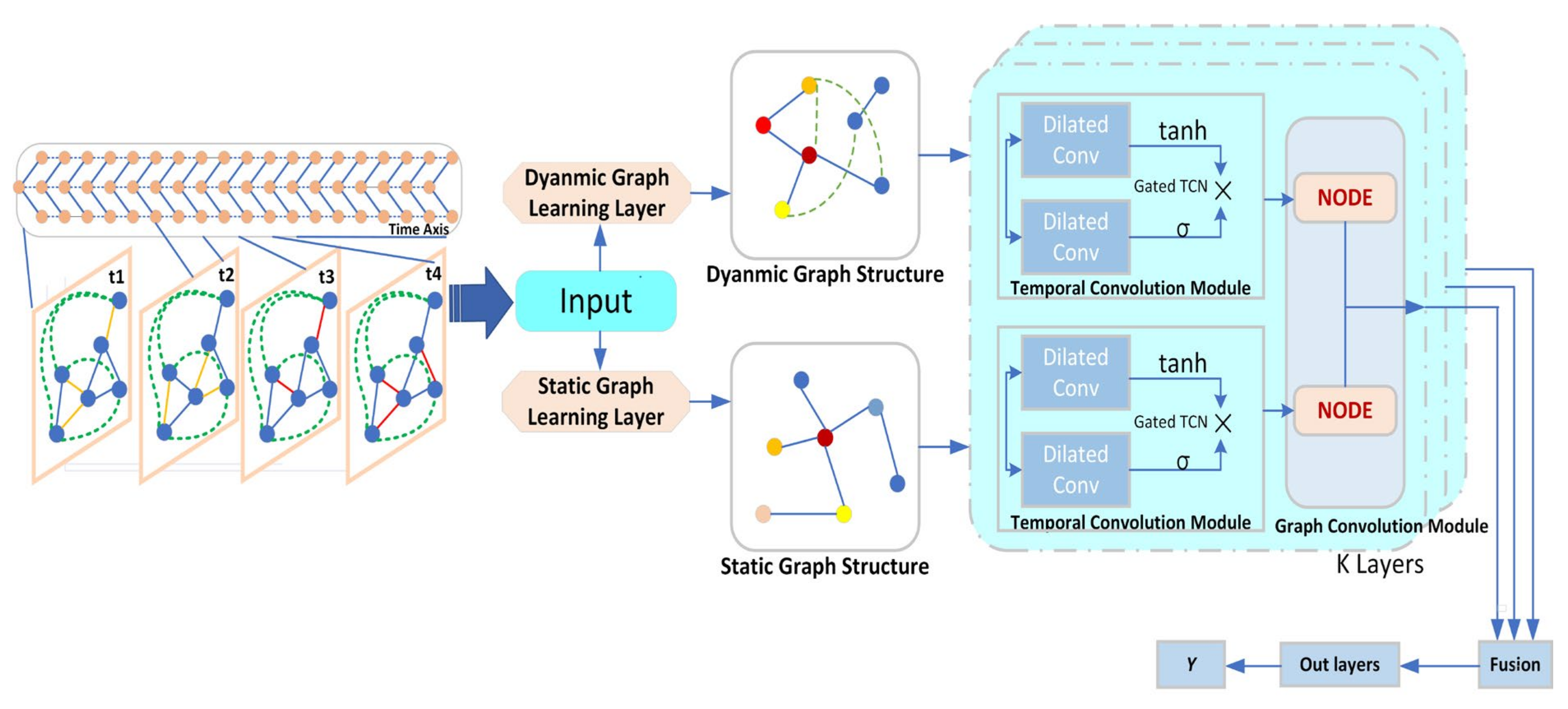
To solve the spatio-temporal dynamics problem in traffic flow, we propose the spatio-temporal dynamic graph ordinary differential equation network (ST-DGDE) framework, as shown in Figure 3. The main framework of the model consists of four modules: dynamic graph learning layer (DGL), static graph learning layer (SGL), temporal convolution module (gated TCN), and dynamic neural graph differential equation (DNGDE) module. The dynamic graph learning layer extracts the dynamic spatial graph structure features hidden in the temporal traffic data and then constructs the generated dynamic graph. The static adjacency matrix is also constructed based on the geographic distance between spatial nodes for auxiliary functions. Then the dynamic and static graphs are fed into the dynamic neural graph ordinary differential equation module in parallel. The distance-based static graph and the node attribute-based dynamic graph reflect the correlation between nodes from different perspectives. Combining the dynamic map with the predefined map gives the model a larger view of the traffic network, thus improving the performance of traffic prediction.

In this paper, we propose a spatial dynamic neural graph differential equation network (GDE) and a graph learning model to learn spatial–temporal dynamic correlations between continuous long time series, which alleviates the reliance on static graph prior knowledge and mitigates the common problem of over-smoothing in GNN construction of deep networks. First, the model learns the continuous fine-grained temporal dynamics between time series through the continuous temporal causal aggregation (TCN) and dynamic graph learning layer (DGL) in the middle part; then, the information of long time series extracted from the temporal convolution module is fed into the differential equation module to learn the hidden dynamic temporal dependencies between continuous time series. Finally, the output of each layer’s dynamic graph differential equation module is used as the input of the next layer module, and the iterative fusion learning results are used as the output.

4.1. Dynamic Graph Learning Layer

Due to the dynamic nature of the traffic road network, there is a dynamic adjustment of the spatial dependencies between different road segments with time. Therefore, in this chapter, dynamic graph constructors are used to capture the different changing relationships between nodes, and they can capture the unstructured patterns hidden in the graph. For traffic networks, the correlations between nodes change over time, and simply applying GCN to traffic networks will not capture this dynamic. For this reason, this chapter employs a dynamic graph learning layer (DGL), which adaptively adjusts correlation strength between nodes. The output vector of the graph learning layer is in continuous space, and its goal is to extract the desired features of the graph.

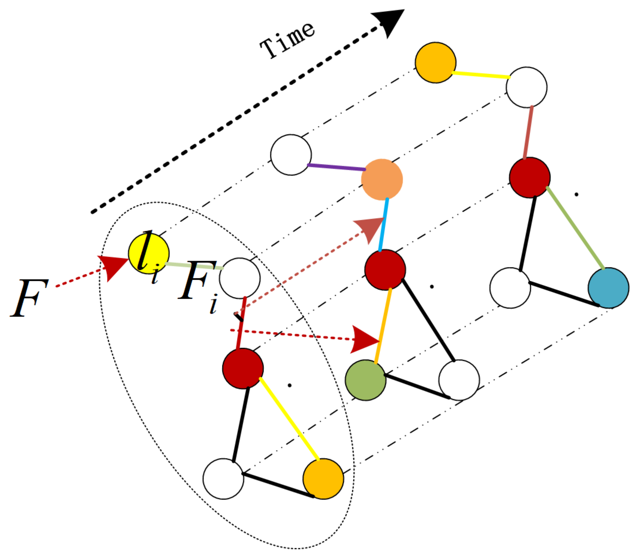
Figure 4 shows that each node is associated with an input label. As time evolves, the correlations between nodes in the spatial graph generated at each time point change. The feature representations of the same observed node at different time points also differ. Therefore, node $v_i$ corresponding label can be denoted as $l_i$. For the dynamic spatial information propagation process, the input graph feature is denoted as $F$, where $F_i$ is the associated feature of node $v_i$. The output feature of the spatial information graph learner at the next moment is denoted as $F^{\prime }$. Equation (3) describes the information propagation process of node $v_i$.

$$F^{\prime }={{\displaystyle \sum }}_{v_{j\in \mathcal{N}\left(v_i\right)}}\mathcal{G}\left(l_i,F_i,l_j\right) ,$$

(3)

In Equation (3), $\mathcal{G}()$ represents a function with parameters called the local transformation function, which is spatially localized, i.e., the information transfer process of node $v_i$ involves only its 1-hop neighbors. When performing the filtering operation, all nodes in the graph share the function $\mathcal{G}()$. Note that the node label information $l_i$ can be considered a fixed initial input information for the filtering process. In Equation (3), $\mathcal{G}()$ represents a function with parameters called the local transformation function, which is spatially localized, i.e., the information transfer process of node $v_i$ involves only its 1-hop neighbors. When performing the filtering operation, all nodes in the graph share the function $\mathcal{G}()$. Note that the node label information $l_i$ can be considered a fixed initial input information for the filtering process.

Static distance-based graphs and dynamic node attribute-based graphs reflect the correlation between nodes from different perspectives. In order to broaden the application of traffic network models, this chapter deploys the graph learning module by combining dynamic graphs with predefined graphs. Moreover, the underlying topology is obtained dynamically using the graph constructor. It is then fed into a gated temporal convolutional network to learn long-range spatial dynamic features by dynamically extracting continuous and more distant message-passing graph structures, thus improving the performance of traffic prediction. In addition, the convolutional structure of TCN combines the historical information with the current moment through a flexible information aggregation approach to extract the temporal and structural information in the dynamic graph, which also unifies temporal and spatial convolution from another perspective.

4.2. Neural Graph Differential Equations (Neural GDEs)

In conventional neural networks, the hidden state is represented by a series of discrete transformations:

$$h\left(t+1\right)=f\left(h\left(t\right),\theta \left(t\right),t\right),$$

(4)

where $f$ is the layer $t$ neural network with parameters $\theta \left(t\right)$, such as $h\left(t+1\right)=\sigma \left(W_{t}h\left(t\right)+b_t\right)$, so that $t$ can also be interpreted as a time coordinate, and the data input x at the moment $t=0$ is transformed into the output $y$ at the moment $t=N$.

Traffic flow time series data are composed of a sparse set of measurements together (the data format in the dataset is an aggregation of data in periods of every five minutes), so these data measurements can be interpreted in terms of many kinds of potentially dynamic processes. Although neural network (NP) [35] models have the characteristics of providing uncertainty estimates and the ability to adapt to the data quickly, they cannot capture dynamic time series features. Therefore, to achieve a dynamic representation of continuous time series, the approach we adopted introduces neural ODE processes (NDPs) [35], a new class of stochastic processes determined by the distribution over the neural ODE. By maintaining adaptive data-dependent distributions on the underlying ODEs, the dynamical processes of low-dimensional systems can be successfully captured from spatiotemporal data. Meanwhile, the ordinary differential equations (ODEs) can effectively capture the underlying spatial–temporal data dynamics and overcome the over-smoothing and over-squeezing problems of graphical neural networks, which in turn can build deep neural network models [36] that can model the time series in traffic flow represented as an ordinary differential equation (ODE).

$$\frac{dh\left(t\right)}{dt}=f\left(h\left(t\right),\theta \left(t\right),t\right),$$

(5)

Given the initial state data of traffic flow $h\left(t_0\right)=x$, the input data are modeled as the rate of change $\frac{dh\left(t_0\right)}{d{t}_0}$ so that the ODE can describe the evolution of the state $h\left(t\right)$ in a given dynamic system with time $t$. As shown in Equation (6), when $f$ is that of a neural network, the equation is considered a neural ordinary differential equation (neural ODE). We can transform a neural ODE into an integral form to obtain $h\left(t\right)$.

$$h\left(t\right)=h\left(t_0\right)+{{\displaystyle \int }}_{t_0}^{t}f\left(h\left(t^{\prime }\right),\theta \left(t^{\prime }\right),t^{\prime }\right)d{t}^{\prime },$$

(6)

CGNN [37] first extends the ordinary differential equations of God to graphical structured data by employing a continuous message-passing layer that portrays the dynamic representation between nodes and thus enables the construction of a deep network. Influenced by this work, we construct the neural graph differential equation network module shown in Figure 5 by fusing graph neural networks with ordinary differential equations based on the dynamic mesh properties of traffic data.

As shown in Figure 5, an example of an ODE solver connecting location observation graphs to prediction graphs is shown. The information on the dynamic changes in the road network from $t_0$ to $t_n$ moments is first learned by the observation function, and the feature maps sampled at each time point are mapped into the potential space by a neural encoder and aggregated into $r$. Then the uncertainty $L$ of the dynamic graph changes and the uncertainty $D$ representation of the ODE derivatives are decomposed by $r$. The ODE solver is designed to define the continuous dynamics of the node representations, where the dynamic long-term dependence between nodes can be efficiently modeled. Since the different nodes in the graph are interconnected, ODE solver considers the structural information in the graph and allows the information to be propagated between different nodes. The way the information is propagated is shown by Equation (7).

$$H_{n+1}=A{H}_n+H_0$$

(7)

$H_n\in R^{\left|V\right|\times d}$ is the spatial embedding matrix of all nodes at time step n. Intuitively, each node at stage $n+1$ learns node information from its neighbors through $A{H}_n$ and remembers its original node features through $H_0$. This allows us to learn the graph structure dynamically without forgetting the original node features.

Given the initial time $t_0$ and the target time point $t_{n+p}$, the neural graph differential equation network (neural GDE) predicts the corresponding state ${\widehat{y}}_{n+P}$ by performing the following integrated encoding and decoding operations:

$$\dot{z}=f_{\theta }\left(z,t\right)$$

(8)

$$z\left(t_n\right)=h_1\left(y_n\right)$$

(9)

$$z\left(t_{n+P}\right)=z\left(t_n\right)+{{\displaystyle \int }}_{t_0}^{t_{n+P}}{f}_{\theta }\left(z\left(t\right),t\right)dt$$

(10)

$${\widehat{y}}_{n+P}=h_2\left(z\left(t_{n+P}\right)\right)$$

(11)

$f_{\theta }$ is a depth-varying vector field function defined on graph G and $\dot{z}$ is denoted as the parameterized velocity of state $z$ at time $t$. $h_1$ and $h_2$ are two affine linear mapping functions on the encoder and decoder, respectively. $h_1$, the mapping function, inputs historical time series observations $y_n$ into the ODE solver to learn continuous dynamic time features. Then, the output $z\left(t_{n+P}\right)$ of the ODE solver is transformed into the predicted future traffic condition ${\widehat{y}}_{n+P}$ by the mapping function $h_2$.

4.3. Gated Temporal Causal Convolutional Networks

Bai S et al. [38] proposed a temporal convolutional neural network (TCN). They experimentally evaluated and demonstrated that temporal convolutional networks (TCNs) are effective in modeling long-time series data and have excellent long-range spatial information capture capability [39]. The TCN architecture is more canonical than LSTM and GRU, and the network model is more straightforward and transparent. Therefore, applying deep networks to time series data may be a suitable starting point.

The TCN network has two distinctive features [40]: on the one hand, the convolution in the model architecture is causal, which effectively avoids “leakage” of future messages; the convolutional computation is also performed layer by layer, with simultaneous updates at each time step, which effectively improves the computational efficiency of the model. On the other hand, the architecture can be mapped to the output sequence using an input sequence of arbitrary length, as in RNN. Therefore, it is possible to use dilated convolution to construct very long effective history sequences, increasing the model’s perceptual field.

The input time is first given in the sequence modeling. The input time sequence ${\widehat{\mathcal{x}}}_0,\cdots ,{\widehat{\mathcal{x}}}_T$ is first given in the sequence modeling. The goal of the model is to predict the output value ${\mathcal{Y}}_0,\cdots ,{\mathcal{Y}}_T$ at each future moment.

$${\widehat{\mathcal{Y}}}_0,\cdots ,{\widehat{\mathcal{Y}}}_T=f\left({\widehat{\mathcal{x}}}_0,\cdots ,{\widehat{\mathcal{x}}}_T\right),$$

(12)

In Equation (11), if the output value ${\widehat{\mathcal{Y}}}_T$ at the future moment satisfies the causal sequence, its input relies only on the input sequence ${\widehat{\mathcal{x}}}_0,\cdots ,{\widehat{\mathcal{x}}}_t$ and not on the future time sequence ${\mathcal{x}}_{t+1},\cdots ,{\mathcal{x}}_T$.

To achieve consistent network input and output lengths, the TCN uses a 1D fully convolutional network (FCN) architecture in which each hidden layer is the same length as the input layer and adds a zero-padding length (kernel size of 1) to keep subsequent layers the same length as previous layers. To avoid future information “leakage,” TCNs use causal convolution, where the output at time $t$ is only convolved with elements from input time t and earlier in the previous layers. For example, the TCN network architecture consists of a 1D FCN and a causal convolution. A significant drawback of this basic design structure is that a deeper network structure is required to capture long-time series information [41]. Therefore, to build deeper networks and capture long-time series information, it is necessary to integrate modern convolutional network architectures into TCNs.

4.4. Module Fusion Output

The ST-DGDE model framework contains one or more blocks, as shown in Figure 3. The computational procedure of the network framework containing L T-DGDE blocks can be expressed as Equation (12).

$$S^{\left(j\right)},D^{\left(j\right)}=B^{\left(j\right)}\left(S^{\left(j-1\right)},D^{\left(j-1\right)}\right), j=1,\dots ,L.,$$

(13)

where $S^{\left(0\right)}=F$ and $D^{\left(0\right)}=A$ denote the adjacency matrix of the static graph and the initial node features of the dynamic graph, respectively. $B^{\left(j\right)}$ denotes the mapping functions that can be learned on each network model layer.

The output of one neural graph differential equation module is the input of the next consecutive block, as shown in Figure 3. When there is only one block, i.e., when $j$ = 1, the ST-DGDE model framework is planar and generates graph-level features directly from the original graph; when L is more significant than 1, the T-DGDE module can be viewed as a hierarchical process that gradually summarizes node features to form predictive graph features by generating smaller, coarsened graphs.

$$\widehat{Y}=W_s\odot S^{\left(j\right)}+W_d\odot D^{\left(j\right)}$$

(14)

where $\odot$ is the Hadamard product, and $W_d$ and $W_s$ learning parameters reflect the degree of influence of static and dynamic graphs on the prediction target. Finally, a two-layer MLP is designed as the output layer to convert the output of the maximum pooling layer into the final prediction.

5. Experiment

This section is optional but can be added to the manuscript if the discussion is unusually long or complex.

5.1. Datasets

As shown in

Table 1. Datasets description.

Datasets	#Node	#Edges	#Time Steps	#Time Range	#Missing Ratio
PEMS04	307	340	16,992	1 January–28 February 2018	3.182%
PEMS08	170	295	17,856	1 July–31 August 2016	0.696%

, the PEMSO4 and PEMS08 data used in the experiments were collected in real time every 30 s by the Caltrans Performance Measurement System (PeMS). The system has over 39,000 detectors deployed on freeways in major California metropolitan areas. The collected traffic data are aggregated into one-time steps every 5 min interval, with 288 time steps for a day’s traffic flow. As shown in Table 1, the total time duration of the PEMS04 data set is 59 days with 16,992 time steps, and the total time duration of the PEMS08 data set is 62 days with 17,856 time steps.

The experiment uses two metrics, including mean absolute error (MAE) and root mean square error (RMSE), to evaluate all methods widely used to assess the accuracy of regression problems. For all metrics, the lower the value, the better. They are defined as

$$MAE\left({\widehat{y}}_i,y_i\right)=\frac{1}{n}{\displaystyle \sum }_{i=1}^n\left|y_i-{\widehat{y}}_i\right|$$

(15)

$$RMSE\left({\widehat{y}}_i,y_i\right)=\sqrt{\frac{1}{n}{\displaystyle \sum }_{i=1}^n{\left(y_i-{\widehat{y}}_i\right)}^2}$$

(16)

5.2. Baseline Methods

To evaluate the performance of our model, we choose eight baselines to compare with.

VAR [8]: Vector autoregressive model is an unstructured system of equations model that captures the pairwise relationships between traffic flow time series.

SVR [10]: Support vector regression uses linear support vector machines to perform the regression task.

DCRNN [30] (Li et al. 2017): Uses bipartite graph random wandering to simulate spatial dependencies and gated recursive units with integrated graph convolution to capture temporal dynamics.

STGCN [19]: Spatial–temporal graph convolution network. Integrates graph convolution into a single convolution unit to capture spatial dependencies.

ASTGCN [38]: Attention mechanism-based spatial–temporal graph convolutional network uses spatial attention and temporal attention to model temporal and spatial dynamic information, respectively.

STSGCN [21]: Spatial–temporal simultaneous graph convolutional network which not only captures local spatial–temporal correlations efficiently but also takes into account the heterogeneity of spatial–temporal data.

LSGCN [34]: Integrating graph attention networks and graph convolutional networks (GCNs) into a spatial gating block, which can effectively capture complex spatial–temporal features and obtain stable prediction results.

5.3. Experimental Parameter Settings

We decompose the PEMS04 and PEMS08 datasets into a training set, a validation set, and a test set in the ratio of 6:2:2 concerning ASTGCN and STSGCN. Specifically, the total time duration of the PEMS04 dataset is 59 days, with 16,992 time steps. Therefore, the first 10,195 time steps are set as the training set, 3398 time steps as the validation set, and 3398 time steps as the test set.

The total time duration of the PEMS08 dataset is 62 days, of which there are 17,856 time steps. The first 10,714 time steps are set as the training set, 3572 time steps as the validation set, and 3572 time steps as the test set. In addition, we normalized the data samples of each road section by the following Equation (6), and the normalized data were input to the model. The model was optimized by inverse mode auto-differentiation and Adam.

$$x^{\prime }=\frac{x-mean\left(x\right)}{std\left(x\right)}$$

(17)

We implement our ST-DGDE model using the PyTorch framework, and all experiments are compiled on a Linux server. All experiments in this paper were conducted in a computer environment with CPU: Intel(R) Core(TM) i7-9900k CPU @ 3.60 GHz and TESLA T4 16G GPU card. We use Adam optimizer to optimize the ST-DGDE model with the number of training iterations set to 200, the batch size to 16, and the learning rate parameter to 0.001.

5.4. Experimental Results and Comparative Analysis

As shown in

Table 2. Shows that our STDGDE model outperforms all baseline results on both datasets.

Baseline Methods		VAR	SVR	DCRNN	STGCN	ASTGCN(r)	STSGCN	LSGCN	STDGDE
Datasets	Metrics
PEMS04	MAE	23.75	28.70	24.63	22.66	22.93	21.19	21.53	20.55
	RMSE	36.66	44.56	37.65	36.01	35.22	33.65	33.86	32.21
PEMS08	MAE	23.46	23.25	17.46	18.11	18.61	17.13	17.73	16.81
	RMSE	36.33	36.16	27.83	27.88	28.16	26.80	26.76	26.12

, our ST-DGDE model is compared with the baseline of the proposed eight methods on two real-world datasets. Table 2 shows the average results of the traffic prediction performance for the next hour.

These experiments will be summarized to answer the following research questions.

RQ1: What is the overall traffic prediction performance of STDGDE compared to the various baselines?

RQ2: How do the different submodules designed improve the model performance?

RQ3: How does the model perform on long-term prediction problems?

RQ4: How do the hyperparameters of the model affect the experimental results?

5.5. Ablation Experiments

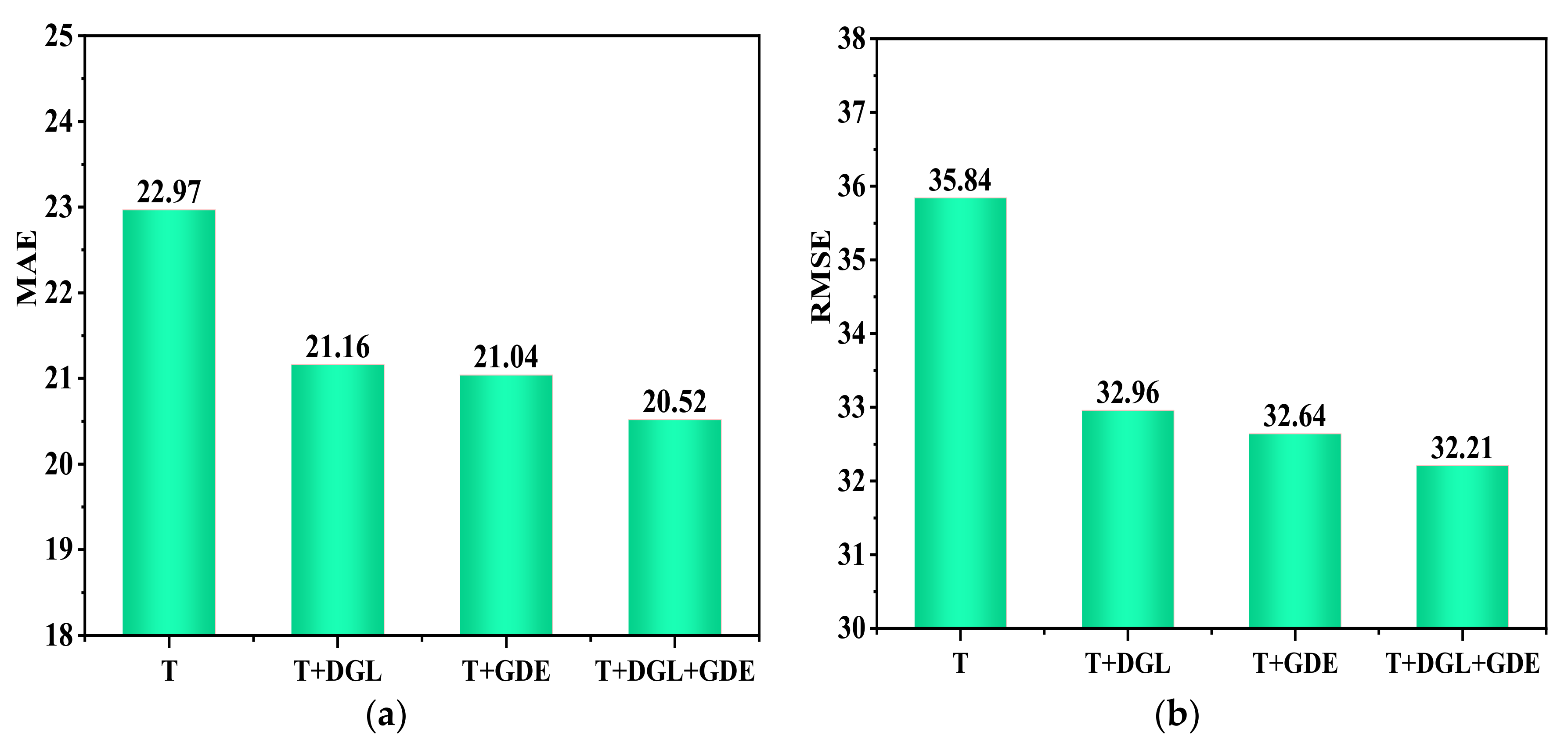
To evaluate the effect of different modules on STDGDE by ablation analysis of the model, we divided the model into three primary modules to test the effect of different modules on the prediction effect of the model separately. For simplicity of representation, we use English abbreviations to denote the module names, which contain three different modules of gated time convolution (T), dynamic graph learning module (DGL), and neural graph differential equations (NGDEs), respectively. In this chapter, we use the PEMS04 dataset to complete the ablation experiments and then analyze the experimental results.

We present the details of the three ablation modules as follows:

T: Gated temporal causal convolution module (Gated TCN).

T + DGL: Adopt T as the base module and add the dynamic graph learning module (DGL) for capturing dynamic change features in spatial–temporal data.

T + NGDE: Adding the neural graph differential equation module to the T module to verify the ability of God’s frequent differential equations to capture hidden dynamic spatial–temporal correlation information.

T + DGL + NGDE: add the neural graph differential equation module to the T + DGL module, which is this chapter model’s spatial–temporal dynamic graph differential equation (STDGDE).

It can be seen from Figure 6 that the STDGDE (T + DGL + NGDE) model in this chapter outperforms other variants in MAE and RMSE evaluation metrics. The result analysis, as shown in Figure 6 (T + DG) data metrics, improves model prediction performance in both MAE and RMSE evaluation metrics when the dynamic graph learning module (DGL) is added. This indicates that the dynamic graph learning module can effectively construct dynamic spatial graphs in the temporal data to improve the model performance. The neural graph differential equations are added separately to the gated temporal causal convolution module, and the spatial perception capability of the model is expanded by combining static and dynamic graph modeling with STDGDE (T + DGL + NGDE) to capture the hidden dynamic spatial–temporal correlations in the data effectively.

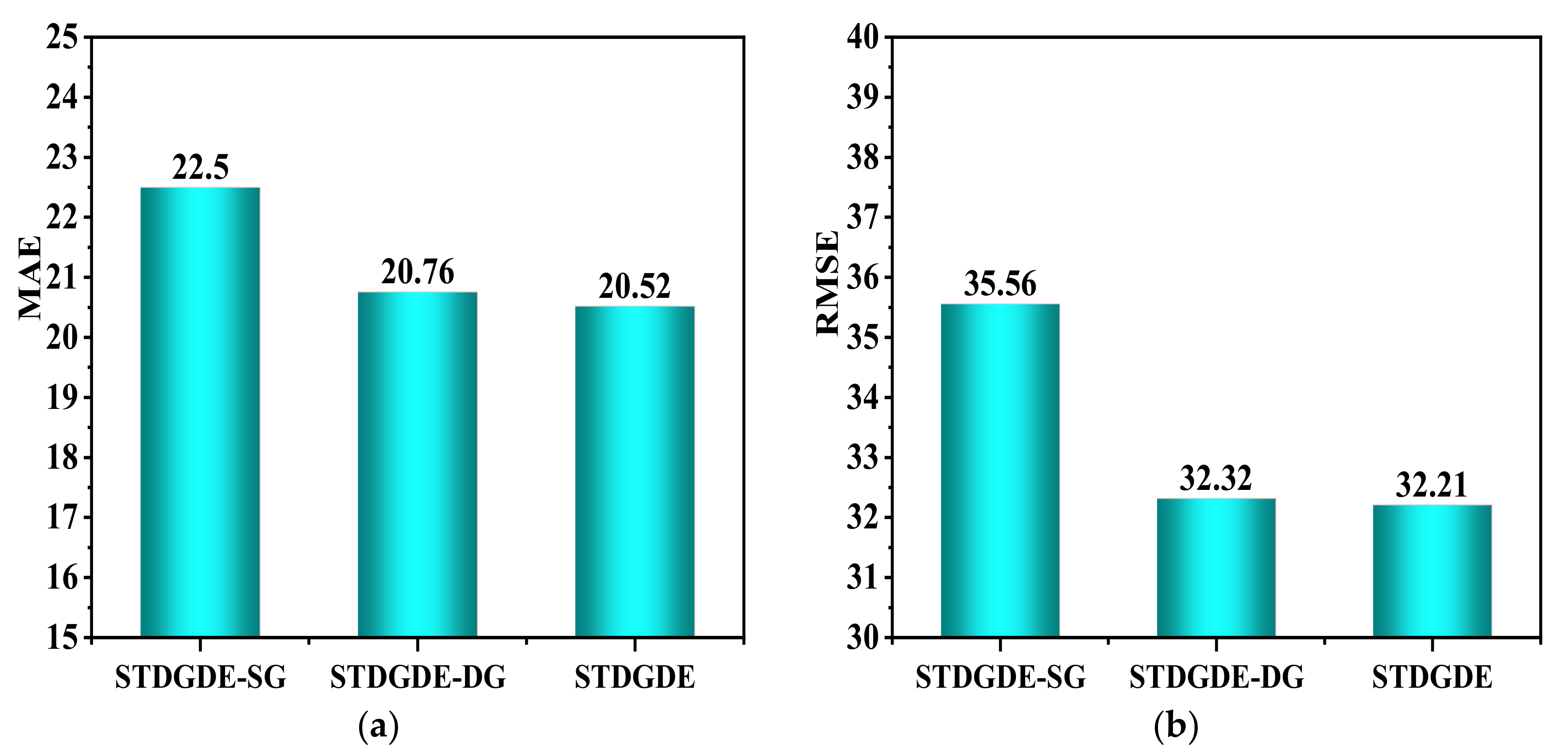
To further analyze the effects of static and dynamic plots on model prediction performance, we conducted ablation experiments on static and dynamic plot modules in the PEMS04 dataset. As shown in Figure 7, STDGDE-SG indicates the use of static plots, and STDGDE-DG indicates the use of static plots.

Figure 7 shows that the prediction effect is greatly improved when the model uses dynamic graphs, indicating that the model can better capture the potential dynamic change information in the data and better accomplish the dynamic prediction task. The comparison indexes of STDGDE and STDGDE-SG in MAE and RMSE data illustrate that static graphs can assist dynamic graph prediction and improve the prediction effect.

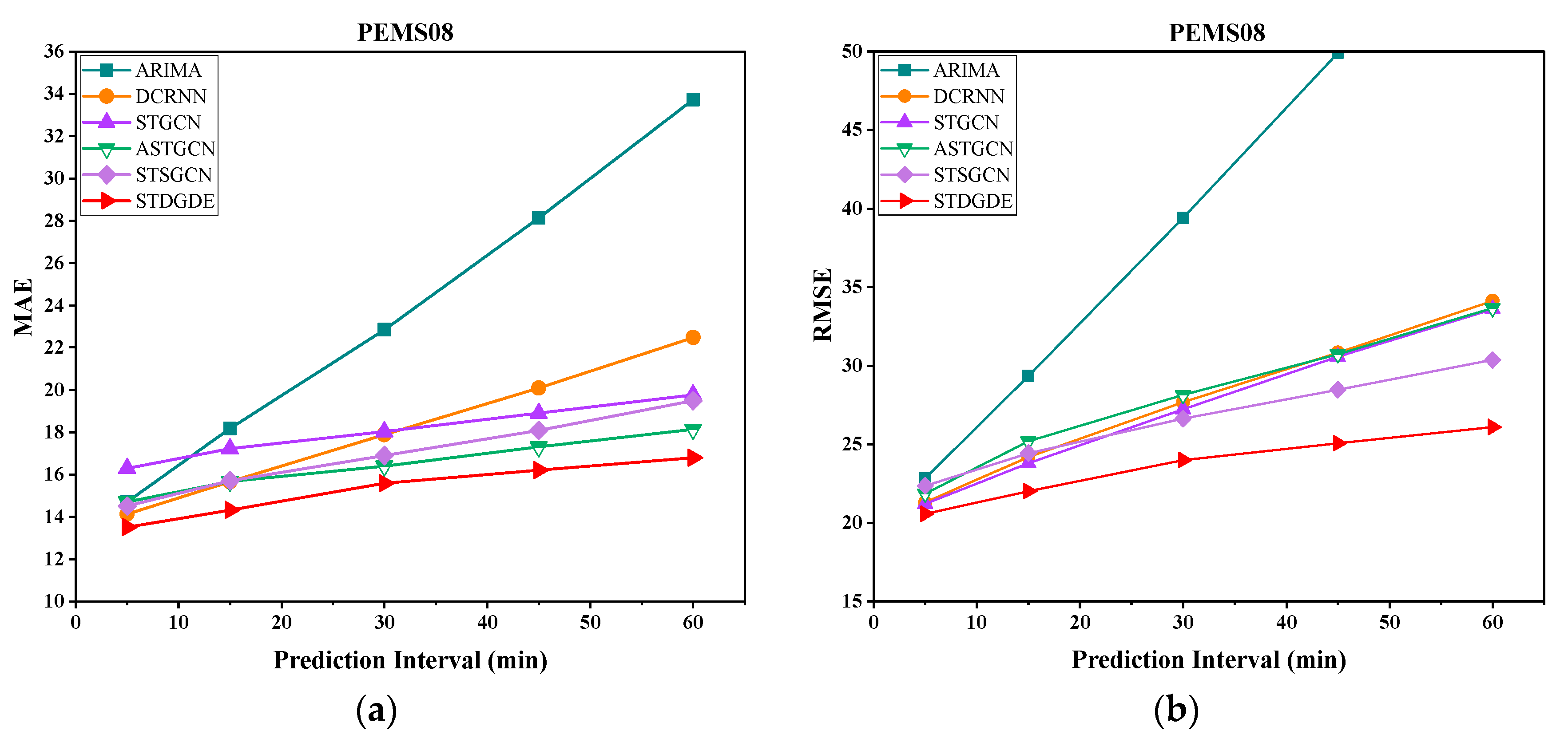
As the prediction time interval increases, the prediction difficulty will also increase, and the model’s prediction performance will decrease. Therefore, in order to investigate the prediction results of the model at different time steps, we show in Figure 8 and Figure 9 the effect of different prediction time intervals on the prediction performance of different methods, and it can be seen that the prediction error of the model increases with the increase in the prediction time length. Our model STDGDE has the best prediction performance at each time step. Additionally, the increase in model prediction error with increasing prediction time length on dataset PEMS04 is relatively slow. The missing data in the PEMS08 dataset leads to poorer prediction results when performing short-term predictions of 5 min and 15 min. However, the model, STDGDE in this chapter, can effectively alleviate the data loss problem in short-term prediction because of the joint capture of spatial–temporal data changes by static and dynamic maps, and the overall stability of the model is better.

6. Conclusions and Future Work

We consider the complex spatial dependence of traffic data and the dynamic spatio-temporal trends among different roads. Thus, we propose a new traffic forecasting framework, the spatio-temporal dynamic graph differential equation network (STDGDE). A neural graph differential equation (NGDE) is designed to complement the missing graph topology and enable spatial and temporal messaging, allowing information propagation in deeper graph networks and fine-grained temporal information aggregation to characterize the underlying spatio-temporal dynamics. Experimental results on the PEMS04 and PEMS08 datasets demonstrate the superior performance of the STDGDE model. The ablation experiments demonstrate the effectiveness of our proposed STDGDE model. In real traffic scenarios, external factors also significantly impact future traffic conditions, such as weather conditions, POI, and road emergencies. Therefore, the following work will collect information on the region’s weather conditions and functional attributes of the area, and this external information will be employed to improve the prediction performance of the model.