Abstract
In recent times, the power sector has become a focal point of extensive scientific interest, driven by a convergence of factors, such as mounting global concerns surrounding climate change, the persistent increase in electricity prices within the wholesale energy market, and the surge in investments catalyzed by technological advancements across diverse sectors. These evolving challenges have necessitated the emergence of new imperatives aimed at effectively managing energy resources, ensuring grid stability, bolstering reliability, and making informed decisions. One area that has garnered particular attention is the accurate prediction of end-user electricity load, which has emerged as a critical facet in the pursuit of efficient energy management. To tackle this challenge, machine and deep learning models have emerged as popular and promising approaches, owing to their having remarkable effectiveness in handling complex time series data. In this paper, the development of an algorithmic model that leverages an automated process to provide highly accurate predictions of electricity load, specifically tailored for the island of Thira in Greece, is introduced. Through the implementation of an automated application, an array of deep learning forecasting models were meticulously crafted, encompassing the Multilayer Perceptron, Long Short-Term Memory (LSTM), One Dimensional Convolutional Neural Network (CNN-1D), hybrid CNN–LSTM, Temporal Convolutional Network (TCN), and an innovative hybrid model called the Convolutional LSTM Encoder–Decoder. Through evaluation of prediction accuracy, satisfactory performance across all the models considered was observed, with the proposed hybrid model showcasing the highest level of accuracy. These findings underscore the profound significance of employing deep learning techniques for precise forecasting of electricity demand, thereby offering valuable insights with which to tackle the multifaceted challenges encountered within the power sector. By adopting advanced forecasting methodologies, the electricity sector moves towards greater efficiency, resilience and sustainability.
Keywords:
load forecasting; long short-term memory; Temporal Convolution Networks; Multilayer Perceptron; Convolutional Neural Networks; CNN–LSTM; Convolutional LSTM Encoder–Decoder; evaluation metrics; power sector; data analysis MSC:
68T07
1. Introduction
The power energy sector is perhaps gathering the most interest from scientists and stakeholders in recent years, due to the rapid development and changes that have occurred. New investments, which create needs for new equipment, but also the establishment of new rules and legislation aimed at protecting the environment and eliminating the greenhouse effect, make this sector more critical and create necessary conditions for its control [1]. At the same time, a wide and extensive energy crisis has been created on a global scale, mainly due to the recent phenomenon of the war that has broken out in Northern Europe. Large industrial units and businesses are suspending their operations due to increased operating costs. With the global increase in electricity demand, the uncertainties and energy risks have also increased [2].
Electrical load forecasting and power generated from different renewable energy sources is extremely important to ensure the performance and effectiveness of all power networks [3,4,5]. This sector is generally classified in terms of forecasting load as follows: very short-term load forecasting (VSLTF) for a few minutes, short-term load forecasting (SLTF) ranging from one hour to one week ahead, mid-term load forecasting (MLTF) for more than one week to a few months and long-term load forecasting (LTLF) for longer than one year [6]. In this work, STLF was used to predict future electrical demand.
In terms of electrical load forecasting, several methodologies have been introduced and can be classified into two main groups of methods: traditional and modern. In traditional techniques, statistical methods are mostly applied. These include models such as autoregression (AR), moving average (MA), autoregressive moving average (ARMA), autoregressive integrated moving average (ARIMA), ARMA and ARIMA with exogenous inputs (ARMAX and ARIMAX, respectively), grey (GM) and exponential smoothing (ES) [7,8].
On the other hand, modern load forecasting methods take advantage of neural networks, which are more suitable for processing complex associations within the data and for developing robust forecasting models that are tolerant to noise. The simplest Artificial Neural Network (ANN) is the MultiLayer Perceptron (MLP) which can model non-linear trends, is able to manage missing values in the datasets, while also providing fast predictions after training [9], as observed by Kontogiannis et al. in trials with household electrical power consumption data. The proposed MLP model, in comparison with LSTM models with several configurations and the 1D CNN model, presents a lower loss function score (mean absolute error) and faster average converge time [10]. Arvanitidis et al. used MLP models to suggest novel train data pre-processing approaches [11] and clustering techniques [12] for SLTF. Furthermore, MLP architecture is extended to conduct day-ahead electricity price forecasting [13].
Moreover, another type of ANNs are the long short-term memory (LSTM) networks, which are capable of identifying the long-term dependencies between data points. In 2017, Zheng et al. [14] presented a hybrid algorithm that combines similar day (SD) selection, Empirical Mode Decomposition (EMD), and LSTM neural networks to construct a prediction model for STLF of ISO New England. This hybrid model, when compared to other forecasting models, showed good effectiveness on SD clustering and accurate forecasting on complex non-linear electric load time series. Additionally, Kwon et al., in 2020 [15], proposed an LSTM model combined with fully-connected (FC) layers, which predicted Korea’s total electrical load. Specifically, the LSTM layer is used to extract the variability and dynamics from historical data, while the FC layers are used to project prediction data and shape the relationship with the output of the layer. The proposed model demonstrated lower load forecasting error (mean absolute percentage error) compared with the STLF method used by Korea’s power operator. Another hybrid model was presented by Jin et al. [16] for real power prediction in three major Australian states, which accomplished high prediction accuracy. The authors, to strengthen the prediction performance, were focused on the importance of the data pre-processing with the variational mode decomposition (VMD) method and conducted an advanced optimization technique with the binary encoding genetic algorithm (BEGA) to optimize the length of the input data sample unit of the LSTM and the number of cell units.
Furthermore, a few studies have found that the LSTM models can be combined with Convolutional Neural Networks (CNNs), which can extract the features of the input data. In 2018, Tian et al. [17] first introduced a new STLF model, which combined CNN and LSTM modules to improve forecasting accuracy. After several detailed experiments were conducted on real world load data from the Italy–North area, the authors concluded that the proposed model improved performance at least 12% and 14%, compared to the individual CNN and LSTM prediction models, respectively. Similarly, Rafi et al. [18] found that the developed CNN–LSTM network provided the lowest values of evaluation metrics compared to LSTM, radial basis functional network and extreme gradient boosting models for short-term load forecasting in the Bangladeshi power system. In [19], the authors studied the forecasting performance of an attention-based CNN combined with LSTM and a bidirectional LSTM model on time-sequenced, non-linear, and complex electrical load data from an integrated energy system park in North China. The examined model and other attention-based LSTM models performed better in predictions than the traditional machine learning models, such as backpropagation neural network (BPNN), random forest regression (RFR) and support vector regression (SVR). Even though the previously mentioned ANN models present exceptional forecast performance, the researchers [20] mentioned that the extracted features of the CNN module influenced the training of LSTM. So, they also suggested a combined CNN and LSTM model wherein the CNN module and LSTM module work in two parallel paths. The processed data then enters a fully connected layer, which includes dense and dropout layers, leading to the final prediction. The suggested framework, named PLCNet, was tested in two case studies for different time horizons and it manifested that this approach had advantages in accuracy and model convergence speed.
In addition to the previously mentioned ANN topologies, recent studies have examined the use of the Temporal Convolutional Network (TCN) model for short-term load forecasting, due to its superiority in long-term feature extraction in time series. Peng and Liu [21] suggested a TCN prediction model for residential short-term load forecasting based on the AMPds2 smart energy meter dataset. The important consumption elements are determined as auxiliary inputs to the prediction model, after a correlation analysis among total load and appliance loads of the household. In terms of prediction performance, the proposed model obtained lower evaluation metrics than the models it was compared with. In [22], the researchers examined a hybrid TCN–LightBGM model, opposed to statistical, deep learning, tree and hybrid models, for a range of industrial consumers. This hybrid model utilized the benefits of TCN in feature extraction and LightGBM in load prediction which improved forecast accuracy in comparison with other models. Other researchers proposed, in [23], a novel STLF model based on TCN and Attention Mechanism (AM), which examines the effect of weather fluctuations on the load forecast and reveals the non-linear association between weather and load data. Additionally, a combination of fuzzy c-means (FCM) clustering algorithm and dynamic time wrapping (DTM) was applied to classify similar power data in clusters. Despite the proposed framework presenting slower training time per epoch than the compared models, due to the requirement for more weight parameters to be trained, it also presented more accurate prediction in terms of evaluation metrics.
The Deep Learning topology we propose in this work for STLF is a hybrid model, named Convolutional LSTM Encoder–Decoder, which was used by other researchers to forecast global total electron content [24] and to predict the El Niño-related Oceanic Niño Index (ONI) and El Niño events [25]. Generally, our research contributions can be summarized as follows:
- Proposal of a hybrid model called Convolutional LSTM Encoder–Decoder for power production time series.
- Presentation of an automated STLF algorithm which incorporates data pre-processing techniques, training, optimization of several AI models, testing and prediction of results.
The remaining part of the paper is organized as follows. Section 2 presents several short-term load forecasting approaches. Section 3 analyzes the dataset, the essential procedures related to the pre-processing of the data used for forecasting, the architecture of the artificial intelligence models and the automated STLF algorithm. In Section 4, the experiments of the case study are illustrated and the results of experiments discussed. Finally, Section 5 contains the conclusions of this work and suggests some directions for future work.
2. Materials and Methods
This section provides a brief and concise description of the fundamental concepts of each of the Deep Learning models used in this paper. More specifically, descriptions for each model are presented.
2.1. Forecasting Approaches
2.1.1. Long Short-Term Memory Networks
Long Short-Term Memory models are variants of the RNN network that overcome the vanishing or explosion of gradients of the latter when processing the long-term dependencies of load series. They were first proposed in 1970 to efficiently handle the long-term dependencies that may exist in time series. Through adding the input, output, and forget gates to the RNN, the LSTM has been widely used in natural language processing (NLP), machine translation, load forecasting and in the health sector.
In regard to the architecture and working principle, the core idea behind the LSTM (Figure 1) and the key operating point is the cell state, which is the horizontal black line at the top of the middle module and the connecting link between the modules [26].
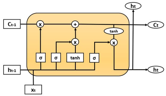
Figure 1.
Basic Structure of LSTM model.
The working mechanism of the LSTM structure, from left to right, is described below:
- Forget Gate (): the useful bits of the cell state (long-term memory of the network) are decided on given both the previous hidden state and new input data . At the bottom, the forget gate controls which part of the long-term memory must be forgotten.
- Input Gate (): The main operation of the input gate is to update the cell state of the LSTM unit. Firstly, a sigmoid layer decides which values it is going to update. Next, a layer creates a vector () of all possible values that can be added to the cell state and, finally, these two are combined to update the cell state.
- Cell State (): The Cell State multiplies the old state by and then adds .
- Output Gate (): The output gate decides what information is going to be output. Using a sigmoid and a tanh function to multiply the two outputs they create, what information the hidden state must carry is decided on.
and represent the weight matrices and biases for the Forget Gate, Input Gate, Cell State, and Output Gate, respectively.
2.1.2. MultiLayer Perceptron
Multilayer Perceptron (MLP) is a type of Deep Learning Feed-forward Neural Network that consists of full connection of hidden layers and has one input and one output layer. The MLP’s architecture is illustrated in Figure 2.
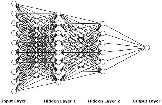
Figure 2.
Basic Multilayer Perceptron Architecture with one input layer, two hidden layers and one output layer.
The process by which MLP algorithms are trained to predict future data is as follows:
- Firstly, MLP algorithms use a Forward Propagation Process to calculate their parameters at the training period, as they propagate data from the input to the output layer.
- Secondly, the network calculates the value of the loss function, which contains the difference between the actual and forecasting data and tries to find the optimal solution, minimizing any error [27].
- Then, using back-propagation algorithms, the gradient of loss function is calculated and the values of the synaptic weights between neurons updated [28].
This process is repeated until the model finds its optimal parameters.
2.1.3. Convolutional Neural Networks
Convolutional Neural Networks (CNNs/ConvNets) are a type of deep learning feed-forward algorithm, originally used for pattern recognition. They are quite similar to conventional neural networks, such as MLPs, since they consist of neurons that contain synaptic weights and biases (learnable weights and biases).
A CNN Model is a sequence of layers. Each CNN neuron receives some inputs and performs a vector operation (dot product). The basic architecture consists of three main types of layers: a Convolutional Layer, a Pooling Layer and a Fully Connected Layer. Each Layer accepts as input a 3D vector and converts it to an output 3D vector through a differentiable function [29]. The main working principle of each of the three main layers are explained below and presented in Figure 3:
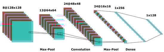
Figure 3.
Main ConvNet Architecture.
- Convolutional Layer: The Convolutional layer is the core building block of a Convolutional Network that does most of the computational heavy lifting.
- Pooling Layer: The objective of the Pooling Layer is the progressive reduction of the spatial size of the representation in order to reduce computational volume of the system and, as a result, to reduce overfitting in the training process.
- Fully-Connected Layer: Neurons in a fully-connected layer have full connections to all activations in the previous layer, as seen in regular Neural Networks. Their activations can, hence, be computed with a matrix multiplication followed by a bias offset.
2.1.4. Hybrid CNN–LSTM Model
The CNN–LSTM model is a hybrid deep learning algorithm that uses the CNN layers for feature extraction of the input dataset and the LSTM model for sequence prediction, resulting in multisteps ahead forecasting of time series. Although the process of this model is divided into two parts, the operation of each of the two component models separately is the same as described in Section 2.1.1 and Section 2.1.3 for LSTM and CNN algorithms, respectively. Figure 4 shows the CNN–LSTM’s architecture.
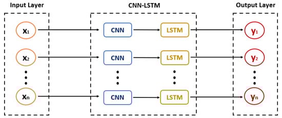
Figure 4.
CNN–LSTM Model Architecture.
2.1.5. Temporal Convolutional Networks
Temporal Convolutional Network (TCN) is a relatively new type of deep learning model that has a dilation of CNN-1D layers, having the same input and output lengths. The working principle of TCNs is the following [30]:
- First, the model computes the low-level features using the CNN-1D modules encoding the spatial–temporal information,
- Second, the model feeds this information and classifies it using Recurrent Neural Networks.
Recent studies have proven that TCNs have great performance in predicting time series with multiple seasonality and trends. Figure 5 presents the basic architecture of a TCN.

Figure 5.
Temporal Convolutional Network [30].
2.2. Proposed Approach: Convolutional LSTM Encoder–Decoder Model
In regard to the proposed model, a description of the Convolutional LSTM Network (ConvLSTM) is first provided and then the basic operation of the Encoder–Decoder Mechanism is analyzed.
The ConvLSTM model uses Recurrent Layers, such as simple RNN and LSTM Networks, but, in contrast with these types of models, the internal matrix multiplications are exchanged with convolutional operations, as this model has convolutional structures in both the input-to-state and state-to-state transitions. As a result, the data that flows through the ConvLSTM cells keeps the input dimension (3D in our case) instead of being just a 1D vector with features [31]. The basic architecture of the ConvLSTM model is presented in Figure 6.
Additionally, the proposed model is a hybrid method that uses an Encoder–Decoder mechanism for the hourly prediction of electricity demand. The Encoder–Decoder mechanism provides efficient techniques for Sequence-to-Sequence (Seq2Seq) forecasting, such as Natural Language Processing (NLP) and time series forecasting, as well as Image Recognition and Sentiment Analysis. An Encoder–Decoder model (Figure 7) consists of three main parts [32]:
- The Encoder Component: This is the first component of the Network and its main function is feature extraction of the input dataset, which is why it is called an ‘encoder’. It receives a sequence as input and passes the information values into the internal state vectors or Encoder Vectors, creating, in this way, a hidden state.
- The Encoder Vector: The encoder vector is the last hidden state of the Network which converts the 2D output of the RNN (ConvLSTM in our case) model to a high length 3D vector in order to help the Decoder Component make better predictions.
- The Decoder Component: The Decoder Component consists of one recurrent unit, or a stack of several recurrent units, each one of which predicts an output y at a time step t.

Figure 6.
A ConvLSTM cell [33].

Figure 7.
Encoder–Decoder Mechanism.
One of the main advantages which makes this model stand out from others is the fact that the input and output vector lengths may be different, allowing this model to perform effectively in big Seq2Seq problems and video captioning.
2.3. Automated STLF Algorithm
Using Deep Learning techniques, a DL-based forecasting algorithm was implemented to easily and efficiently find the best forecasting model for every kind of time series dataset. The function of the algorithm includes the following steps:
- The algorithm loads the dataset.
- The algorithm proceeds to the Pre-processing Step, in which the dataset is normalized using the Min–Max Scaling algorithm, and the Cyclical Time Features are created using One-Hot Encoding.
- The dataset is split into Training, Validation and Test sets.
- Every Deep Learning Model is trained and evaluated using the Bayesian Optimization Algorithm.
- The best model from the algorithm, in terms of higher prediction accuracy, is selected to be used for future predictions.
The algorithmic process is described in Figure 8.
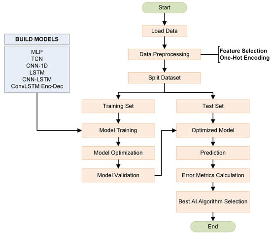
Figure 8.
STLF automated algorithm structure.
3. Case Study
In this section, we present the case study used to test the proposed approach. The final dataset used for our experiments incorporated weather conditions and power demand from the Greek Cycladic Island, in the Aegean Sea, Thira, also known as Santorini. Thira island is a non-interconnected island to the Greek electrical bulk network and the power production is solely based on fossil fuel generators. The dataset period was three years from January 2017 to December 2019. The specific time period was chosen because the power requirements followed a normal distribution and there were no special events (such as COVID-19) that would hinder safe conclusions. Working with this dataset, no such limitations were observed. Regarding the challenges encountered, these came mainly from the parameterization and adaptation of the algorithms created and their abilities to be assimilated and trained on a dataset with multiple seasonality, such as the one studied.
3.1. Climate Dataset
The climate data was collected from Santorini airport’s Meteorological Aerodrome Reports (METAR) [34,35]. The airport’s International Civil Aviation Organization (ICAO) code is LGSR. A typical report is usually published from the airport’s weather station every hour or half-hour and aggregates actual values and current conditions for temperature, dew point, wind direction and speed, precipitation, cloud cover and height, visibility, and barometric pressure. For the current work we retrieved, from METARs, hourly values for temperature in °C, dewpoint in °C, wind speed in m/s and degrees of wind direction. Interpolation was applied to fill in missing values in the climate data.
3.2. Electrical Power Dataset and Exploratory Analysis
The power production dataset contained the actual hourly generated energy from the island’s unique thermal station and referred to the entire island’s power demand [36]. Thira exhibits multiple seasonality throughout year, due to changes in the numbers of residents and tourists on the island, which dramatically affects the energy demands of different months. Additionally, the current energy dataset presented nil number of missing values, which facilitated realistic experiments and safe conclusions.
Table 1 presents a descriptive analysis of the power consumption data set. Based on the above table, it can be observed that the dataset contained a total of 25,944 values. Its mean value and standard deviation were 23.31 MW and 9.95 MW, respectively. The minimum value was 8.50 MW and the maximum 51.52 MW. Finally, regarding the intermediate values, it turned out that 25% of the dataset values were smaller than 14.70 MW, 50% smaller than 21.15 MW and 75% smaller than 31 MW, respectively.

Table 1.
Power consumption descriptive analysis.
In order to better observe the daily distribution of power consumption, a boxplot was created. Figure 9 presents the variation of average hourly power per day. It is worth noting that the peak demand was at 01:00 p.m. and 08:00 p.m. every day. The events were more intense on summer days, due to the increased number of tourists on the island.
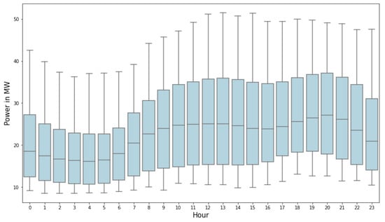
Figure 9.
Boxplot of the daily average hourly consumption for the reviewed time period.
Correlation Heatmap
Figure 10 presents the Correlation Heatmap which visualizes the strength of relationships between all the numerical variables created. For instance, it was clear that the “temperature” variable had a very strong relationship with the “power” variable, which was equal to 0.81 with a maximum possible value of 1.
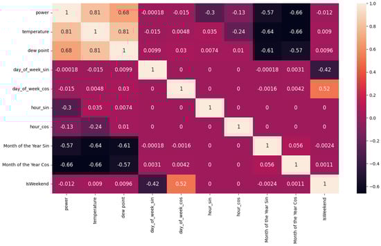
Figure 10.
Feature Correlation Heatmap.
3.3. Feature Selection
Several input features were studied and evaluated for this study to understand the most significant for predicting electricity demand. A total of ten input features were studied for predicting electricity demand one hour ahead. The data used as input variables were the same for all the Deep Learning Models and are shown in Table 2:
Table 2.
Deep learning models’ input variables.
3.4. Data Pre-Possessing
3.4.1. Min–Max Scaling
The prepossessing technique for all the datasets used in this paper was Min–Max Scaling, which scaled all the data points between 0–1. For this reason, two different scalers were used, one for input datasets and one for output datasets. The mathematical formulation is given in the follow equation:
where is the real value of a data, and and are the minimum and maximum values of the dataset, accordingly. The main reason Min–Max Scaling was used is that it helps train the deep learning models more efficiently in the training period and converges faster to an optimal solution of the loss function.
3.4.2. One-Hot Encoding
One-Hot encoding is a mathematical methodology that converts categorical to numerical vectors and transforms numerical data to cyclical data, using trigonometric transformation. Using this technique, day of the week, hour of the day and also month of the year were converted to Sine and Cosine types.
3.5. Data Partitioning
The data was split into training and test sets, while maintaining the temporal order of the data. The data from 1 January 2017 to 30 September 2019, were used as the training set and the last 10% of this were used for the validation of the models. The data from 1 October 2019 to 31 December 2019, were used as the test set. The specific interval was not random. It was chosen because throughout its range it had both an interval with a trend and an interval which was stationary. Thus, the deep learning models were tested in the most difficult case that could be extracted from our dataset. Figure 11 presents the visualization plot of the power consumption for all the datasets and the individual partitioning sections.
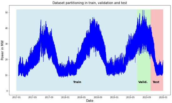
Figure 11.
Dataset partitioning in training, validation and test sets.
3.6. Model Architecture
This subsection details the architectures of each model used in this paper, in order to provide a clear understanding of the optimal parameters that were extracted. The hyperparameters of all models were chosen after applying the Bayesian Hyperparameter Optimization Algorithm with a maximum of 20 iterations in every search. Initially, several trials were performed with different values of batch sizes. Due to the faster convergence and higher accuracy of the DL algorithms, a batch size equal to 128 was chosen for every model created in this paper. The main architectural components and the search space of every hyperparameter optimized for each model are presented in Table 3. The optimal extracted parameters are presented below:
Table 3.
Models main optimization parameters summary.
3.6.1. LSTM Model
The LSTM model performed most accurately in the optimization process and had the following hyperparameters:
- Units of lstm network = 256
- Batch size = 128
- ReLU activation function for the LSTM Module, as well as the output Dense Layer
- Optimizer = Adam
- Learning rate = 0.0010
- Epochs = 100
3.6.2. CNN–LSTM Model
The hyperparameters of the hybrid CNN–LSTM model are presented below:
- filters = 64
- kernel size = 2
- ReLU activation function for the both the CNN and LSTM Module
- 48 units for the LSTM Module
- MaxPooling1D with pool size = 2
- Batch size = 128
- Optimizer = Adam
- Learning rate = 0.0010
- Epochs = 100
3.6.3. Multilayer Perceptron Model
After converging to the optimal forecasting accuracy, the hyperparameters for the MLP model were formulated as follow:
- 480 Neurons for the Input Layer
- Batch size = 128
- ReLU activation function for the Input Layer, as well as the output Dense Layer
- Optimizer = Adam
- Learning rate = 0.0011
- Epochs = 100
3.6.4. Temporal Convolution Network
- Filters = 256
- Dilations = [1, 2, 4, 8, 16, 32]
- Batch size = 128
- Optimizer = Adam
- Learning rate = 0.0010
- Epochs = 100
3.6.5. CNN-1D Model
- Filters = 64
- Kernel size = 3
- MaxPooling1D (pool size = 2)
- Neurons of Dense Layer = 16
- ReLU activation function for the CNN Module, as well as the output Dense Layer
- Optimizer = Adam
- Learning rate = 0.0010
- Epochs = 100
3.6.6. ConvLSTM Encoder–Decoder Model
This is this paper’s proposed hybrid model, which outperformed the other deep learning models. The hyperparameters that composed the architecture of this model were the followings:
- Filters = 64
- Kernel size = (1,4)
- ReLU activation function for the ConvLSTM2D Module, for the LSTM Layer, as well as the output Dense Layer
- Encoder Vector with size = 1
- 64 Units for the LSTM module
- Optimizer = Adam
- Learning rate = 0.0068
- Epochs = 100
A visualization of each model is presented in Figure 12.
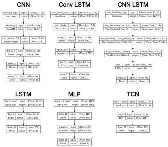
Figure 12.
Models visualization.
3.7. Software Environment
The experiments presented in this study were implemented in Python 3.8 Language, using the Open-Source software library Tensorflow 2.11.0 and the high-level API, Keras 2.11.0. Pandas 1.5.2 and Numpy 1.23.5 libraries were used for data analysis and visualization of the problem. The project was executed on Google Colab Pro platform, using a GPU with the following characteristics: NVIDIA- SMI 460.32.03, Driver Version: 460.32.03, CUDA Version: 11.2, RAM: 25.45 GB and Disk: 166.77 GB.
Regarding the time required to train each model, one of the primary factors influencing this process is the architecture and the level of complexity of each model, and, more specifically, the number of trainable parameters required to train each algorithm. Among the models examined, the MLP (MultiLayer Perceptron) stood out as the simplest and fastest to train, followed by CNN-1D, CNN–LSTM, LSTM, ConvLSTM Encoder–Decoder, and TCN. Despite their architectural differences, the training times did not exhibit significant variations. Once the optimization procedure was completed and the optimal hyperparameters for each algorithm determined, the training of each model took no more than 20 min. Finally, regarding the time required for each model to make a complete prediction, i.e., the inference time, this did not exceed 1 min. So, this remarkably short training time enabled real-time predictions using these models, extending their applicabilities beyond the academic realm pursued in this paper.
3.8. Performance Metrics (Evaluation Metrics)
In this section, we present the performance metrics used in the evaluation of the hourly power prediction models. Mean Absolute Error (MAE) [37] is a commonly used metric with regression models, comparing actual and predicted values, which gives a measure of average error. MAE is calculated by the following formula:
where is the predicted value and is the actual value in a set of n samples.
Moreover, Mean Absolute Percentage Error (MAPE) [38] is used as a measure of quality for regression and time series models because it intuitively explains the relative error. MAPE is computed by the following formula, which uses the same parameters as the MAE calculation:
Furthermore, Mean Squared Error (MSE) [37] and Root Mean Squared Error (RMSE) [39] metrics were included in the performance evaluation of this study. The MSE metric measures the average squared difference between the predicted and true values. In this study, we used MSE as the loss function for the training of the neural network prediction models, due to its characteristic of giving a higher weight on extreme error values. MSE and RMSE metrics, which use the same parameters as the previously mentioned evaluation metrics, are given as follows:
Additionally, the coefficient of determination, or R squared, was used as a performance metric in this study, representing the proportion of variance (of y), explained by the independent variables in the model. It indicates a proper model fit and measures how possible it is for unobserved samples to be forecast by the model, through the proportion of explained variance. R squared can be more informative than the formerly mentioned metrics in regression analysis evaluation [39]. R squared is calculated by the following formula:
where is the predicted value, is the actual value and is the mean of the actual values in a set of n samples.
4. Results Analysis and Discussion
In the presented work, an automated application was implemented in order to find the optimal forecasting model for hourly electricity data in MWs. For this purpose, six artificial deep learning models were created and optimized, as shown in the tables above. Essentially, an application was implemented which is not only able to run on electric power data, but can also be used in any kind of time series forecasting problems.
The results obtained from the algorithmic experiments are presented and an analysis of their results conducted. In Figure 13 the prediction of the daily hourly demand in MWs for a three-month period, from 1 October 2019 to 31 December 2019, is presented.
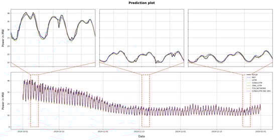
Figure 13.
The prediction results. Lower subfigure represents the whole testing dataset. Upper subfigures describe different three-day prediction plots from the same training dataset.
More specifically, Table 4 presents the values of R2, MAE, MSE, RMSE and MAPE for each model. For a better understanding of the results, the above table was sorted by MAPE in descending order and the optimal metrics’ values are presented in bold.
Table 4.
Evaluation metrics.
Based on the experiments carried out, it is easy to see that the worst models were the CNN-1D and TCN networks. The models containing Recurrent Networks, such as LSTM and the two hybrid models implemented, were the most accurate. So, an important finding was that the models that contain only convolutional operations were the least accurate, a fact that led to the conclusion that such a mechanism does not allow models to extract meaningful features from input time series data, compared to other models.
More specifically, the CNN-1D and TCN models presented MAE 0.4936 and 0.4576 MW and RMSE 0.7282 and 0.7096 MW, respectively, while the MLP model achieved MAE equal to 0.4477 and RMSE equal to 0.6784 MW. The LSTM model presented MAE 0.4275 and RMSE 0.6747 MW and the hybrid CNN–LSTM network presented MAE 0.4412 and RMSE 0.6866 MW, respectively.
The proposed model, which has not been extensively used in electricity forecasting datasets, is a hybrid model, called Convolutional LSTM Encoder–Decoder. The advantage of this model, compared to the other models implemented and particularly compared to the hybrid CNN–LSTM model, is the use of a ConvLSTM Network, offering better feature extraction and accuracy. Thus, the profile of a time series with multiple seasonality, such as the one studied in our case, is recognized in a more efficient way, making this model capable of achieving MAE and RMSE 0.4142 and 0.6674, respectively. Figure 14 presents and illustrates the comparative values of R2, MAE, MSE and RMSE for each of the six models proposed.
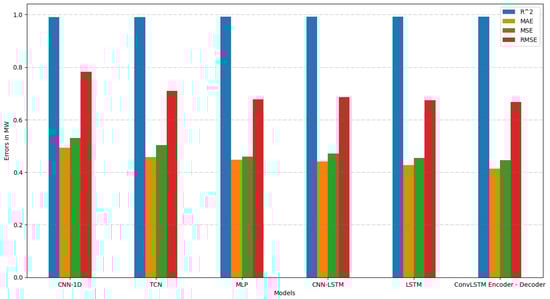
Figure 14.
Comparison of the models in terms of R2, MAE, MSE and RMSE error metrics.
5. Conclusions and Future Work
In recent years, the energy sector has experienced substantial transformations due to a continuous surge in demand and to energy crises. These developments have given rise to new requirements aimed at addressing emerging situations and ensuring the effective and efficient operation of the power grid. Accurate demand forecasting is a key factor for the reliable operation and robustness of modern power systems. In short-term load forecasting, efficiency is a cornerstone for market flexibility which ensures balance between supply and consumption in real time. For these reasons, this study introduced an innovative and automated Deep Learning forecasting model for use in the energy sector. The load forecasting results of five enhanced models, namely, the CNN-1D, LSTM, CNN–LSTM, TCN and MLP, were ascertained and compared with those generated by the proposed forecasting hybrid model, named ConvLSTM Encoder–Decoder.
Based on the results obtained and presented, the proposed ConvLSTM Encoder–Decoder, compared with the other methods, had better results, achieving a MAPE equal to 2.15%. The LSTM followed with 2.25%, the hybrid CNN–LSTM with 2.31%, MLP with 2.38%, TCN with 2.40% and, lastly, CNN-1D, with a MAPE equal to 2.66%. The differences in terms of the MAPE were quite small among the models, most likely due to the extensive optimization process carried out for all models.
Regarding the contribution of the current research, it emphasizes the benefits in implementing a Deep Learning automated algorithm, capable of identifying the optimal model in predicting future time series data across various problems. While the present study focused on load forecasting, the proposed approach could also be applied to predict quantities in systems involving renewable energy sources, such as wind and solar power. Moreover, the system has potential in predicting building energy consumption in general and, specifically, in commercial, industrial and military facilities, considering factors such as climate data, indoor environmental information and occupants’ behavior, which applies to time series problems.
In addition, through the suggested load forecasting model, a new and innovative deep learning model is presented that achieved the higher forecasting accuracy among the models studied. This proposed hybrid model consists of a ConvLSTM component, which encodes the information contained in the input time series vectors. Then, the information passes through an Encoder Vector, and is distributed to an LSTM model, targeted to predict future data.
Considering the aforementioned contribution of the current research, it is apparent that the developed methodology distinguishes itself from its counterparts presented in the literature review. While the referenced papers primarily focused on comparing outcomes derived from various statistical and machine learning methods, this work adopted a different approach. The selection of the best model was accomplished through an automated process, introducing flexibility and performance for potential users of the developed application. Furthermore, an advantage of the proposed approach lies in the introduction of a state-of-the-art model (ConvLSTM Encoder–Decoder) that has not been applied extensively before to load forecasting problems.
In terms of future research directions stemming from the current research, some noteworthy propositions emerge. The automated model could be enhanced by incorporating additional efficient models, such as the Exponential Smoothing LSTM (ESLSTM) and advanced Multi-Head Transformer. A notable challenge lies in applying the models developed to medium- and long-term multistep prediction tasks to evaluate their stability over extended sequences. Furthermore, testing the applicability of the proposed approach in regard to other diverse types of time series data, could also be a significant challenge. Moreover, conducting a comparative analysis of prediction accuracy in time series tasks by combining the models used in this paper with Custom Activation Functions represents another potential avenue for future investigation. Lastly, exploring the utilization of these algorithms in Demand Side Management and Demand Response problems is a challenging prospect, given the high level of accuracy required for short-term forecasting in such problems.
Author Contributions
Conceptualization, V.L. and G.V.; methodology, V.L.; software, V.L. and G.V.; validation, V.L., G.V., D.B., A.D. and L.H.T.; formal analysis, V.L. and G.V.; investigation, V.L. and G.V.; resources, V.L. and G.V.; data curation, V.L. and G.V.; writing—original draft preparation, V.L. and G.V.; writing—review and editing, V.L., G.V., D.B., A.D. and L.H.T.; visualization, V.L. and G.V.; supervision, D.B., A.D. and L.H.T.; project administration, D.B. and A.D. All authors have read and agreed to the published version of the manuscript.
Funding
This research received no external funding.
Institutional Review Board Statement
Not applicable.
Informed Consent Statement
Not applicable.
Data Availability Statement
Data are available in a publicly accessible repository. The load data used in this study are available from the HEDNO portal in [36]. The weather dataset was retrieved from ogimet portal in [35]. These datasets were processed as the input for the design and performance assessment of the forecasting models described in this article.
Conflicts of Interest
The authors declare no conflict of interest.
Abbreviations
The following abbreviations are used in this manuscript:
| AM | Attention Mechanism |
| BO | Bayesian Optimization |
| BEGA | Binary Encoding Genetic Algorithm |
| BPNN | Backpropagation Neural Network |
| CNN-1d | Convolutional Neural Network One Dimensional |
| CNN-LSTM | Convolutional Neural Network—Long Short-Term Memory |
| ConvLSTM | Convolutional Long Short-Term Memory |
| DTM | Dynamic Time Wrapping |
| FC | Fully-Connected |
| LSTM | Long Short-Term Memory |
| MAE | Mean Absolute Error |
| MAPE | Mean Absolute Percentage Error |
| MLP | Multilayer Perceptron |
| NLP | Natural language processing |
| R2 | R-Squared |
| RFR | Random Forests Regression |
| RMSE | Root Mean Squared Error |
| RNN | Recurrent Neural Network |
| STLF | Short-Term Load Forecasting |
| SVR | Support Vector Regression |
| TCN | Temporal Convolutional Network |
References
- Karthik, N.; Parvathy, A.K.; Arul, R.; Padmanathan, K. Multi-objective optimal power flow using a new heuristic optimization algorithm with the incorporation of renewable energy sources. Int. J. Energy Environ. Eng. 2021, 12, 641–678. [Google Scholar] [CrossRef]
- Laitsos, V.M.; Bargiotas, D.; Daskalopulu, A.; Arvanitidis, A.I.; Tsoukalas, L.H. An incentive-based implementation of demand side management in power systems. Energies 2021, 14, 7994. [Google Scholar] [CrossRef]
- Poongavanam, E.; Kasinathan, P.; Kanagasabai, K. Optimal Energy Forecasting Using Hybrid Recurrent Neural Networks. Intell. Autom. Soft Comput. 2023, 36, 249–265. [Google Scholar] [CrossRef]
- Arvanitidis, A.I.; Kontogiannis, D.; Vontzos, G.; Laitsos, V.; Bargiotas, D. Stochastic Heuristic Optimization of Machine Learning Estimators for Short-Term Wind Power Forecasting. In Proceedings of the IEEE 2022 57th International Universities Power Engineering Conference (UPEC), Istanbul, Turkey, 30 August–2 September 2022; pp. 1–6. [Google Scholar] [CrossRef]
- Vontzos, G.; Bargiotas, D. A Regional Civilian Airport Model at Remote Island for Smart Grid Simulation. In Proceedings of the Smart Energy for Smart Transport: Proceedings of the 6th Conference on Sustainable Urban Mobility, CSUM2022, Skiathos Island, Greece, 31 August–2 September 2022; Springer: Berlin/Heidelberg, Germany, 2023; pp. 183–192. [Google Scholar] [CrossRef]
- Mamun, A.A.; Sohel, M.; Mohammad, N.; Haque Sunny, M.S.; Dipta, D.R.; Hossain, E. A Comprehensive Review of the Load Forecasting Techniques Using Single and Hybrid Predictive Models. IEEE Access 2020, 8, 134911–134939. [Google Scholar] [CrossRef]
- Hammad, M.A.; Jereb, B.; Rosi, B.; Dragan, D. Methods and models for electric load forecasting: A comprehensive review. Logist. Supply Chain. Sustain. Glob. Chall. 2020, 11, 51–76. [Google Scholar] [CrossRef]
- Hong, T.; Fan, S. Probabilistic electric load forecasting: A tutorial review. Int. J. Forecast. 2016, 32, 914–938. [Google Scholar] [CrossRef]
- Deep Learning Tutorial for Beginners: Neural Network Basics. Available online: https://www.guru99.com/deep-learning-tutorial.html{#}5 (accessed on 18 November 2022).
- Kontogiannis, D.; Bargiotas, D.; Daskalopulu, A. Minutely active power forecasting models using Neural Networks. Sustainability 2020, 12, 3177. [Google Scholar] [CrossRef]
- Arvanitidis, A.I.; Bargiotas, D.; Daskalopulu, A.; Laitsos, V.M.; Tsoukalas, L.H. Enhanced Short-Term Load Forecasting Using Artificial Neural Networks. Energies 2021, 14, 7788. [Google Scholar] [CrossRef]
- Arvanitidis, A.I.; Bargiotas, D.; Daskalopulu, A.; Kontogiannis, D.; Panapakidis, I.P.; Tsoukalas, L.H. Clustering Informed MLP Models for Fast and Accurate Short-Term Load Forecasting. Energies 2022, 15, 1295. [Google Scholar] [CrossRef]
- Kontogiannis, D.; Bargiotas, D.; Daskalopulu, A.; Arvanitidis, A.I.; Tsoukalas, L.H. Error compensation enhanced day-ahead electricity price forecasting. Energies 2022, 15, 1466. [Google Scholar] [CrossRef]
- Zheng, H.; Yuan, J.; Chen, L. Short-term load forecasting using EMD-LSTM neural networks with a Xgboost algorithm for feature importance evaluation. Energies 2017, 10, 1168. [Google Scholar] [CrossRef]
- Kwon, B.S.; Park, R.J.; Song, K.B. Short-term load forecasting based on deep neural networks using LSTM layer. J. Electr. Eng. Technol. 2020, 15, 1501–1509. [Google Scholar] [CrossRef]
- Jin, Y.; Guo, H.; Wang, J.; Song, A. A hybrid system based on LSTM for short-term power load forecasting. Energies 2020, 13, 6241. [Google Scholar] [CrossRef]
- Tian, C.; Ma, J.; Zhang, C.; Zhan, P. A deep neural network model for short-term load forecast based on long short-term memory network and convolutional neural network. Energies 2018, 11, 3493. [Google Scholar] [CrossRef]
- Rafi, S.H.; Nahid-Al-Masood; Deeba, S.R.; Hossain, E. A Short-Term Load Forecasting Method Using Integrated CNN and LSTM Network. IEEE Access 2021, 9, 32436–32448. [Google Scholar] [CrossRef]
- Wu, K.; Wu, J.; Feng, L.; Yang, B.; Liang, R.; Yang, S.; Zhao, R. An attention-based CNN-LSTM-BiLSTM model for short-term electric load forecasting in integrated energy system. Int. Trans. Electr. Energy Syst. 2021, 31, e12637. [Google Scholar] [CrossRef]
- Farsi, B.; Amayri, M.; Bouguila, N.; Eicker, U. On Short-Term Load Forecasting Using Machine Learning Techniques and a Novel Parallel Deep LSTM-CNN Approach. IEEE Access 2021, 9, 31191–31212. [Google Scholar] [CrossRef]
- Peng, Q.; Liu, Z.W. Short-Term Residential Load Forecasting Based on Smart Meter Data Using Temporal Convolutional Networks. In Proceedings of the IEEE 2020 39th Chinese Control Conference (CCC), Shenyang, China, 27–29 July 2020; pp. 5423–5428. [Google Scholar] [CrossRef]
- Wang, Y.; Chen, J.; Chen, X.; Zeng, X.; Kong, Y.; Sun, S.; Guo, Y.; Liu, Y. Short-Term Load Forecasting for Industrial Customers Based on TCN-LightGBM. IEEE Trans. Power Syst. 2021, 36, 1984–1997. [Google Scholar] [CrossRef]
- Tang, X.; Chen, H.; Xiang, W.; Yang, J.; Zou, M. Short-term load forecasting using channel and temporal attention based temporal convolutional network. Electr. Power Syst. Res. 2022, 205, 107761. [Google Scholar] [CrossRef]
- Xia, G.; Zhang, F.; Wang, C.; Zhou, C. ED-ConvLSTM: A Novel Global Ionospheric Total Electron Content Medium-Term Forecast Model. Space Weather 2022, 20, e2021SW002959. [Google Scholar] [CrossRef]
- Wang, S.; Mu, L.; Liu, D. A hybrid approach for El Niño prediction based on Empirical Mode Decomposition and convolutional LSTM Encoder-Decoder. Comput. Geosci. 2021, 149, 104695. [Google Scholar] [CrossRef]
- Olah, C. Understanding LSTM Networks. Available online: https://colah.github.io/posts/2015-08-Understanding-LSTMs/ (accessed on 12 January 2023).
- Banoula, M. An Overview on Multilayer Perceptron (MLP). Available online: https://www.simplilearn.com/tutorials/deep-learning-tutorial/multilayer-perceptron#forward_propagation (accessed on 7 January 2023).
- Andrew Zola, J.V. What Is a Backpropagation Algorithm? Available online: https://www.techtarget.com/searchenterpriseai/definition/backpropagation-algorithm (accessed on 7 January 2023).
- CS231n Convolutional Neural Networks for Visual Recognition. Available online: https://cs231n.github.io/convolutional-networks/#fc (accessed on 7 January 2023).
- Lara-Benítez, P.; Carranza-García, M.; Luna-Romera, J.M.; Riquelme, J.C. Temporal convolutional networks applied to energy-related time series forecasting. Appl. Sci. 2020, 10, 2322. [Google Scholar] [CrossRef]
- Tian, H.; Chen, J. Deep Learning with Spatial Attention-Based CONV-LSTM for SOC Estimation of Lithium-Ion Batteries. Processes 2022, 10, 2185. [Google Scholar] [CrossRef]
- Brownlee, J. How Does Attention Work in Encoder-Decoder Recurrent Neural Networks. Available online: https://machinelearningmastery.com/how-does-attention-work-in-encoder-decoder-recurrent-neural-networks/ (accessed on 12 January 2023).
- Kim, K.S.; Lee, J.B.; Roh, M.I.; Han, K.M.; Lee, G.H. Prediction of ocean weather based on denoising autoencoder and convolutional LSTM. J. Mar. Sci. Eng. 2020, 8, 805. [Google Scholar] [CrossRef]
- METAR-Wikipedia. Available online: https://en.wikipedia.org/wiki/METAR (accessed on 12 January 2023).
- Ogimet. Available online: https://www.ogimet.com/home.phtml.en (accessed on 12 January 2023).
- Thira ES-HEDNO. Available online: https://deddie.gr/en/themata-tou-diaxeiristi-mi-diasundedemenwn-nisiwn/leitourgia-mdn/dimosieusi-imerisiou-energeiakou-programmatismou/thira-es/ (accessed on 10 January 2022).
- Sammut, C.; Webb, G.I. (Eds.) Encyclopedia of Machine Learning; Springer: Boston, MA, USA, 2010; pp. 652–653. [Google Scholar] [CrossRef]
- De Myttenaere, A.; Golden, B.; Le Grand, B.; Rossi, F. Mean Absolute Percentage Error for regression models. Neurocomputing 2016, 192, 38–48. [Google Scholar] [CrossRef]
- Chicco, D.; Warrens, M.J.; Jurman, G. The coefficient of determination R-squared is more informative than SMAPE, MAE, MAPE, MSE and RMSE in regression analysis evaluation. PeerJ Comput. Sci. 2021, 7, e623. [Google Scholar] [CrossRef]
Disclaimer/Publisher’s Note: The statements, opinions and data contained in all publications are solely those of the individual author(s) and contributor(s) and not of MDPI and/or the editor(s). MDPI and/or the editor(s) disclaim responsibility for any injury to people or property resulting from any ideas, methods, instructions or products referred to in the content. |
© 2023 by the authors. Licensee MDPI, Basel, Switzerland. This article is an open access article distributed under the terms and conditions of the Creative Commons Attribution (CC BY) license (https://creativecommons.org/licenses/by/4.0/).