Abstract
In real-world applications, many problems involve two or more conflicting objectives that need to be optimized at the same time. These are called multi-objective optimization problems (MOPs). To solve these problems, we introduced a guided multi-objective equilibrium optimizer (GMOEO) algorithm based on the equilibrium optimizer (EO), which was inspired by control–volume–mass balance models that use particles (solutions) and their respective concentrations (positions) as search agents in the search space. The GMOEO algorithm involves the integration of an external archive that acts as a guide and stores the optimal Pareto set during the exploration and exploitation of the search space. The key candidate population also acted as a guide, and Pareto dominance was employed to obtain the non-dominated solutions. The principal of -dominance was employed to update the archive solutions, such that they could then guide the particles to ensure better exploration and diversity during the optimization process. Furthermore, we utilized the fast non-dominated sort (FNS) and crowding distance methods for updating the position of the particles efficiently in order to guarantee fast convergence in the direction of the Pareto optimal set and to maintain diversity. The GMOEO algorithm obtained a set of solutions that achieved the best compromise among the competing objectives. GMOEO was tested and validated against various benchmarks, namely the ZDT and DTLZ test functions. Furthermore, a benchmarking study was conducted using cone--dominance as an update strategy for the archive solutions. In addition, several well-known multi-objective algorithms, such as the multi-objective particle-swarm optimization (MOPSO) and the multi-objective grey-wolf optimization (MOGWO), were compared to the proposed algorithm. The experimental results proved definitively that the proposed GMOEO algorithm is a powerful tool for solving MOPs.
Keywords:
metaheuristic algorithms; multi-objective optimization; equilibrium optimizer; Pareto solution set; ϵ-dominance relation; cone-ϵ-dominance MSC:
68T27
1. Introduction
A number of real-life problems have typically been interpreted as optimization problems with multiple conflicting objectives [1,2] (e.g., water distribution networks (WDNs) [3], the traveling salesman problem [4], and protein structures [5]). We are in an era where such problems are increasing daily [6]. In addition, today’s decision-making problems require us to consider large models of these NP-hard problems, both in terms of the number of variables and constraints [7,8,9]. Therefore, these problems are handled and modeled as multi-objective optimization problems (MOPs), where the goal is to find the best set of trade-off solutions—known as a Pareto optimal set or non-dominated solutions [10]. In other words, this type of optimization searches for acceptable compromises between objectives—as compared to single-objective optimization, which is where only one solution has to be found. Therefore, significant attention has been given to this concept, and many works have been proposed [11,12]. Meta-heuristics and evolutionary algorithms have been widely adopted for solving some of the multi-objective optimization problems, including non-dominating sort genetic algorithms (NSGAIIs) [13], where fast non-dominated sorting was used. The extension of NSGAII, called NSGAIII [14], employed a non-dominated sort and a reference point method. The PAES [15] and SPEA2 [16] employed an external archive to store the non-dominated solutions; as such, algorithms have been quite successful and are still used today [17,18].
MOPs have been the most common problems in several real-world applications [19,20]. Therefore, this field has continued to evolve, thus ensuring that many other algorithms were developed, such as the multi-objective evolutionary algorithm based on decomposition (MOEAD) [21], where the problem is decomposed into a number of sub-problems and each one is treated as a single-objective problem. Deb et al. [22] introduced the -MOEA algorithm, where the -dominance relation was employed. Many other extensions of MOEA have been proposed, including the uniform decomposition measurement (UMOEA/D) [23], the MO-memetic algorithm (MOEA/D-SQA) [24], and many others [25,26].
In terms of meta-heuristics algorithms and, particularly, population-based algorithms, algorithms that handle multi-objective problems (MOPs) have typically been an extension of a single-objective-optimization algorithms but modeled in a way to solve MOPs. One of the most well-known algorithms is the multi-objective particle swarm optimization (MOPSO) method, which is based on the single-objective optimization algorithm type of particle swarm optimization (PSO) [27]; it is a population-based algorithm inspired by the biological behavior of birds in a flock. The PSO has been proven to be a successful algorithm that continues to be used for solving optimization problems [28]. Many extended multi-objective versions of the PSO have been proposed. For instance, the swarm metaphor, as proposed in [29], incorporated the Pareto dominance concept and crowding distances. In a different work by Cello et al. [30], another MOPSO was proposed that incorporated a respiratory system to conserve the non-dominated solutions and to choose an instructor that would guide the particles. The well-known algorithm of ant colony optimization (ACO) and its variants [31,32] is another population-based algorithm. It was inspired by ant behavior and designed to solve single-objective optimization problems. Furthermore, it was improved to handle with MOPs accordingly, as in [33,34,35].
Following the same concept over the years, several other MOP algorithms were developed by simply extending the single-objective version [36,37]. The cat swarm optimization (CSO) [38] method was extended by incorporating a Pareto ranking; thus, it was then named the multi-objective cat-swarm optimization (MOCSO) [39]. The grey wolf optimizer (GWO) [40], for example, was also extended by adding an external fixed-size archive, resulting in the multi-objective grey wolf optimization (MOGWO) [41] method. Zouache et al. [42] introduced a guided multi-objective moth–flame optimization (MOMFO) method, which was an extension of the moth–flame optimizer (MFO) [43]. In MFO, an unlimited external archive was used to determine the non-dominated solutions, and the fast non-dominated sort was adopted, along with crowding distances. Furthermore, -dominance was employed as an updated archive strategy. A more recent work attempted to solve MOPs using EO by proposing a multi-objective equilibrium optimizer with an exploration–exploitation dominance strategy (MOEO-EED) [44].
Recently, an equilibrium optimizer algorithm was presented to solve a single-objective optimization problem [45]. The presented results of this algorithm showed that it was able to outperform well-known algorithms. In this paper, based on the aforementioned analysis and the extended versions, we present an extended version of EO called the guided multi-objective equilibrium optimizer (GMOEO), which we used to solve MOPs. The proposed extension employs an external archive through which to obtain the non-dominated solutions and the crowding distances. In addition, it utilizes an exploration–-exploitation dominance, which is where the solutions update was controlled.Furthermore, a Gaussian-based mutation strategy was suggested to boost the exploration and enhance the exploitation. In this work, as compared with MOEO-EED, we attempted to approach the concept using simple strategies.
The main contributions of this paper are summarized as follows.
- We propose a GMOEO method to solve multi-objective optimization problems;
- We incorporated an external archive to store the non-dominated solutions and to guide the particles toward the optimal Pareto set.
- -dominance was employed to update the archive solutions and to ensure improved diversity, exploitation, and exploration. In addition, cone--dominance was employed to update the archive solutions, and was compared with the -dominance relation;
- A fast non-dominating sort and crowding distances were introduced to preserve the diversity and to ensure the convergence of the particles, as well as to ensure an efficient solution distribution;
- The effectiveness of the proposed algorithm was validated through comprehensive experiments conducted on different benchmarks, including ZDT and DTLZ test functions. The performance was then compared with the known multi-objective optimization algorithms.
The rest of the paper is organized as follows. Section 2 explains the basics of multi-objective optimization problems, Pareto optimality, and EO. Section 3 introduces the proposed GMOEO algorithm. The experimental results, comparisons, and discussion are presented in Section 4. Finally, Section 5 contains the conclusions and suggestions for future research directions.
2. Background Information
2.1. Multi-Objective Optimization Problems
Multi-objective optimization is the systematic process of simultaneously collecting and optimizing conflicting objective functions. The optimization could involve minimization or maximization, depending on the problem. A minimization problem could be formulated as follows:
where , , and represent the decision functions of a vector , and refers to decision variables. The variables M, , N, and L refer to the objective functions, search space, the numbers of inequality, and equality constraints, respectively. In an MOP, it was difficult to compare the obtained solutions with the relational arithmetic operators. Therefore, the concept of Pareto optimal dominance provided a simple way through which to compare solutions in the multi-objective search space. Furthermore, there was a set of Pareto optimal solutions with a Pareto front image in the search space, rather than a single optimal solution.
2.2. Pareto Dominance and Optimality
The main concept of the Pareto dominance relation comprised the following:
Definition 1 (Pareto dominance).
Let z and s be two solutions, where z dominates the other solution s (denote as ), iff:
Solution z weakly dominated the other solution s (denoted as ), iff:
Definition 2 (A non-dominated set).
The unique dominant solution where there is no other solution that dominates them. Let D be a set of solutions, such that the non-dominated solutions are members of the set and are not dominated by any other solution in set D.
Definition 3.
The Pareto solution is an optimal solution if it does not become dominated by other solutions in the feasible search space.
 s ∈ x|z ≺ s
Definition 4 (Pareto optimal set).
A set of all non-dominated solutions in the search space.
2.3. Equilibrium Optimizer (EO)
The equilibrium optimization algorithm [45] has recently been introduced to solve optimization problems. The original innovation behind this algorithm was the control–volume–mass balance models, where the mass-balance equation was employed for describing the concentration of a non-reactive constituent in the control volume. It is a first-order differential equation that could provide an understanding of the physics behind the conservation of mass as it enters and leaves the control volume. The solutions represent the particles, while the concentrations represent the positions—similar to PSO. These particles act as a search agent for reaching the optimal solution, which is the equilibrium state. Some of EO’s key parameters that distinguish it from other algorithms include the following: an equilibrium pool and a candidate; a generation rate; and updating process for the particles’ positions.
The steps of the equilibrium optimizer are summarized in Algorithm 1. Similar to other optimization algorithms, the EO began with the initialization of a random population. As a unique approach, EO employed four of the best-so-far candidates and as the equilibrium state, which were not initially known. These candidates were necessary to determine the search pattern for the particles, to assist in the exploration of the search space, and to participate in the update process. In addition to the four candidates, an average candidate was calculated. The equilibrium pool was one of the key benefits of this optimizer, and the elements used in the construction of this vector were the five candidates , which were chosen arbitrarily. This pool participated in updating the concentration (position), where a random candidate would be chosen. Other parameters, such as the generation-rate-control parameter and the generation probability , were also employed. These two parameters contributed to the construction of the generation rate G, which was another key parameter in the EO algorithm. was used to determine the potential contribution of G during the update process, while was used to determine which particle would update its status by using the generation term.
| Algorithm 1 Equilibrium optimizer (EO) [45] |
| Initialize the particles |
| Assign equilibrium candidates’ fitness a large number |
| Assign the parameters , , |
| while Iteration < Maxiteration do |
 |
| end |
The generation rate G is one of the most important terms in the EO algorithm for providing the exact solution, which is achieved by improving the exploitation phase. In engineering applications, there are many models that can be used to express the generation rate as a function of time t. For example, one multi-purpose model that describes generation rates as a first-order exponential decay process is defined as
where is the initial value and k indicates a decay constant. To have a more controlled and systematic search pattern, and to limit the number of random variables, this paper assumes , as well as uses the same previously derived exponential term. Thus, the final set of generation rate is
The time t is defined as a function of iteration, and is provided in Algorithm 1. More details about the parameters, conditions, and mechanisms used in the EO are provided in [45].
3. The Guided Multi-Objective Equilibrium Optimization
The main concept of the proposed guided multi-objective equilibrium optimization (GMOEO) algorithm was the adoption of an external archive in order to store the discovered non-dominated solutions. The non-dominated solutions were obtained via the Pareto-dominance relation and the crowding distance that improved the diversity and the fast non-dominated sort, which assisted in generating the multiple Pareto fronts. Moreover, the -dominance relation was introduced for the purpose of updating the archive solutions. Therefore, the best solutions were used to update the archive, and those solutions were from a candidate population that contained the best solutions of the previous population, as well as the current archive solutions. We also used cone--dominance to update the archive population solution in order to establish a comparison between these two approaches. Finally, the archive was used to guide the particles in the search space toward the optimal front. To summarize, the adopted strategy in the proposed GMOEO incorporated several important aspects:
- An external archive that could store the best non-dominated solutions in order to guide the particles toward the optimal set;
- The use of an efficient -dominance/cone--dominance relation for updating the archive solutions;
- The integration of a candidate population that enhanced the diversity;
- The use of the fast non-dominated sort (FNS) and the crowding distance to ensure an efficient and diverse set of solutions with an efficient convergence toward the Pareto optimal.
Each of these aspects give the proposed GMOEO a great advantage in being a good tool for optimization, i.e., the archive first helps guide the solution, as well as helps to preserve the diversity of the solutions, which helps with gaining a good set of solutions and also in keeping the balance between exploration and exploitation. The -dominance relation allows flexibility and diversity, which helps with including a wide range of solutions. The candidate population is a key point for the exploration and exploitation process. Finally, FNS and the crowding distance are the key tools through which to boost the convergence toward the Pareto optimal and coverage.
After the initialization of the population and the evaluation with respect to the M objectives, we first applied the fast non-dominated sort (FNS) on the first population, and then the crowding distance was applied with the aim of recovering the best solutions. Those solutions were the main elements of our candidate population. Next, the GMOEO used an external archive, called the archive population, which was initialized with the non-dominated solution of the first particle population. This archive retained the best solution, or the non-dominated set, during the whole optimization process, including the exploration of the search space. Furthermore, the archive would be used to guide the particles in a later step. To attain the Pareto set solutions during each iteration, the GMOEO had to conduct the following steps: update the candidate population; update the archive population; and, finally, conduct the particle position update.
3.1. Updating the Candidate Population
As previously mentioned, the candidate population was the basis for updating the archive. In other words, this population contributed to the diversity and convergence toward the Pareto optimal set. In a later step, the EO would use four candidates to manage the movement of the particles. However, in this study, we used the population of the candidates, as this population’s candidates were the non-dominated solutions obtained by applying the FNS and the crowding distance. The solutions of this population were guided by a set of two populations during the exploration and exploitation of the search space during the course of the iterations, resulting in a double population. We combined the previous particle population and the current archive population into one population; therefore, these two populations highly contributed to the diversity and the convergence. After combining these two populations, the FNS was considered to preserve the best solutions resulting from both populations. Then, the crowding distance was computed on the last level of the non-dominated solutions. The large distances were selected to complete the candidate population. The three key parameters used to update the candidate population were the following:
3.1.1. Double Population
Double population was one of the key parameters in the update process. As previously stated, the candidate population was updated using two other populations, which included the previous particle population to maintain the diversity. In addition, during exploration and exploitation, the current archive population was utilized to ensure the convergence. The combination of these two distinguishing populations highly contributed to the convergence toward the Pareto optimal set. Furthermore, it aided in avoiding a premature convergence or stagnation in the local optimum set.
where is the previous particle population and represents the current archive populations.
3.1.2. Sorting
Once the double population was obtained, the improved version of FNS [13] was used to compare each solution individually with the rest, rather that storing the results, to avoid duplicate comparisons between the solutions. Then, it sorted the solutions according to the rank of the non-dominated solutions. Furthermore, FNS was employed to sort and maintain the convergence of the double-population solutions. First, the FNS employed each solution of the double population to test its dominance against the other solutions, which resulted in the first non-dominated front. Next, to obtain the individuals of the next front, the first-front solutions were excluded, and the process was repeated until all the possible subsequent fronts were found.
Within this context, each solution for the double population had two inputs: the number of solutions , which dominated the ith solution, and a set of solutions , which were dominated by the ith solution. For , its solution was assigned to the sub-front . For all the solutions of the current front , every solution of the set traveled, and its count was decreased. However, if , then this solution was set to another sub-set H. After reviewing all of the individuals of the current front, was then announced as the first front. This process was repeated in subset H. Lastly, these solutions were saved based on their front, as is described in Algorithm 2.
This mechanism was employed for estimating the density of a certain solution, which preserved the diversity and supported an efficient distributed solution. The crowding distance that was applied on the population was determined by the application of FNS. The crowding distance was computed as the average distances of two neighboring solutions by considering the respective objectives from all sides. Figure 1 shows the crowding distance of a solution i as the average distance of the cuboid, and is represented by the two closest neighbors and . The solutions were ranked in ascending order based on their crowding distances in objective m. Then, the boundary solutions with the highest and lowest objective values were set to be infinity. The steps of the crowding distance are outlined in Algorithm 3. It should be noted that represents the mth objective function associate with the ith solution in front of F. Once the crowding distance values had been obtained, the solutions were then ranked according to the crowding distance values, and the first n solutions were selected as the new candidate population.
| Algorithm 2 Steps of the fast non-dominated sort algorithm. |
| Input: Double population |
| foreachx ∈ Double population do |
 |
| end |
| Algorithm 3 Steps to compute crowding distance for each solution. |
| Input: F population based Front; |
| N solutions number in the front F |
| foreach k initialize the distance by Zero do |
 |
| end |

Figure 1.
Crowding distance calculation.
3.2. Updating the Archive Population
In order to ensure the performance of the proposed GMOEO, an external archive was used. This archive assisted in maintaining the non-dominated solution and cooperated in the movement of the particles toward the Pareto front. In other words, this archive acted as the equilibrium pool. Two benchmarking strategies were adapted for updating the archive’s solutions: first, we considered the -dominance as an update strategy; second, we employed the cone--dominance.
3.2.1. ϵ-Dominance
The -dominance [46] basically adapted two main mechanisms: box-level and regular dominance. It began as -dominance splits the objective space into hyper-boxes, where each box contained one unique identification vector B for every solution from the archive population . Then, the candidate population —where for the M objectives—was determined by the following:
where is the objective value of the ith solution and refers to the admissible error. Once the identification vectors values were computed, each candidate population solution was then compared to all the archive solutions, which was based on the -dominance relation, to determine whether to add the solution to the archive. The box-level dominance was conducted to ensure the diversity. If the identification vector of the candidate population solution, denoted as , dominated an identification vector of the archive solution, denoted as , then c would be stored in the archive and the archive solution would be removed. Otherwise (i.e., if was dominated by a ), the c solution would not be stored. If neither result occurred, a second mechanism was employed, i.e., a regular dominance . If c dominated , then c would be accepted. If there was no clearly dominant solution, then the closest solution to B would be accepted. Algorithm 4 describes the procedure for updating the archive using -dominance.
| Algorithm 4 Archive updating using ϵ-dominance. |
| Input: Archive population , iteration number t, candidate population c solution. |
| Calculate vector and for all archive population solutions , |
| if then |
 |
| end |
The main reason behind the choice of -dominance is first Pareto optimality, which is the -dominance relation that can provide a Pareto optimal set in a conflicting objectives space. -dominance uses the parameter , which allows for tolerance and flexibility while choosing the optimal solutions that are reflected in the diversity of the solutions. By setting , there is is possibility to obtain different ranks for the solutions in the optimal set. Moreover, -dominance is scalable, and it can handle problems with a large number of objectives. Lastly, this relation is computationally efficient since the comparison involves only two solutions at a time.
3.2.2. Cone-ϵ-Dominance
Cone-ϵ-dominance [47] is a relaxed version of Pareto dominance, which itselfis a relaxed dominance approach. Relaxed dominance [48] was introduced to handle situations such as when a solution has a significantly inferior value to one of the objectives. However, it was not dominated in this study. The -dominance was adopted, and to select the non-dominated solutions with more flexibility, it used linear trade-off functions and set an upper and lower rate between the two distinguishing objectives. Then, it could permit solutions to dominate each other with a significant superiority in only one objective. Consequently, a significant superiority in another objective would typically be rejected by a regular Pareto dominance. Based on the relaxed dominance, cone--dominance was a hybridization of both the -dominance and the -dominance. It attempted to retain the convergence of -dominance while controlling the dominant region using cones.
Definition 5 (Cone).
A set H was indicated as a cone Cone if λ x ∈ H for any x ∈ H ∀ λ ≥ 0.
Definition 6 (Generated Cone).
For two vectors denoted by and , the cone generated by these two vectors is a set H described by the following:
For m dimension, , and , the set H becomes
With respect to the origin of the box and , the cone would then be determined, as follows:
where is a parameter to control the cone opening and ψ is the cone-dominance matrix.
Similar to -dominance, the cone--dominance splits the objective spaces into hyper-boxes. In addition, it adapts two levels of dominance: regular Pareto and box level. The box-level dominance contained one unique identification vector b with upper and lower bounds, such as the property adapted by -dominance. Every solution from the archive population and the candidate population was assigned a box where b would be calculated using the following:
where x represents a solution , which returns the closest low integer to their argument, and returns the closest high integer to their argument.
To add a solution to the archive, a box-level dominance was conducted. Let and be the two identification vectors of the candidate population solution and the archive population solution, respectively. Furthermore, was the cone--dominate if, and only if, was the Pareto dominate ; otherwise, the solution to the linear system was , as determined by the following:
such that
Similarly, if, and only if:
For the identification vectors with the same box, a regular Pareto dominance was employed, where the archive solution would be replaced only if the candidate solution was a Pareto dominant. Otherwise, the closest point to the origin of the box was selected. Algorithm 5 shows the procedure for updating the archive using the cone--dominance.
The cone--dominance relation is as efficient as the -dominance relation; however, it offers more flexibility in defining the region around a solution. In addition cone--dominance allows more accurate representation and coverage.
3.2.3. Evaluating the Archive Population Size
During archive updating, the total number of the solutions can be increased, which would then expand the archive. Therefore, to control the number of the solutions contained in the archive population, we utilized the FNS strategy on the archive population. Then, the crowding distance values computed for the solutions were sorted in descending order, and only the first 100 solutions from this were retained.
| Algorithm 5 Archive updating using the cone ϵ-dominance. |
| Input: Archive population A, candidate population solution |
| Calculate vector and b for all archive population solutions A |
| if c is cone-ϵ-dominated by any then |
 |
| end |
3.3. Updating the Particle Position
The strategy for updating the particle positions, adapted for the GMOEO algorithm, was the same as in EO, as given in Algorithm 1 for updating the concentrations. The only difference in this step was that, instead of using an equilibrium pool with only five candidates, a pool that contained those five candidate in addition to the archive population was used. As a result, we could guarantee the convergence toward the Pareto optimal since the archive contained non-dominated solutions. Algorithm 6 describes the process for updating the particle positions. Using GMOEO for each particle, a solution was randomly selected from the equilibrium pool, i.e., the archive population and the five candidates, and was used in the update process.
| Algorithm 6 Updating particles position. |
| Input: Particles population P, |
| Archive population , |
| =(+++)/4, |
| Equilibrium pool construction: |
| =,,,, |
| for i = 1: number of particles (n) do |
 |
| end |
For the computational complexity of GMOEO, we let N be the size of the population and M the number of objectives. The main loop of the algorithm had the same complexity as the EO [45]. It used a polynomial order of , where t is the number of iteration, c is the cost function, and d is the problem dimension. The first operation was FNS, which had a complexity of . The second operation was the crowding distance of complexity . Finally, updating the archive required the use of -dominance, where the complexity of the operation was , and for the cone--dominance, the complexity was . Consequently, the processing time of the GMOEO algorithm was , , , ]. However, the complexity of GMOEO was , which showed the same complexity as MOPSO [30] and MOGWO [41]. Algorithm 7 illustrates all the steps of the GMOEO with the additional operations. In addition, Figure 2 displays the flowchart for the proposed GMOEO.
| Algorithm 7 The guided multi-objective equilibrium optimizer (GMOEO). |
| Initialize the particles , |
| Assign equilibrium candidates’ fitness a large number, |
| Assign the parameters , , |
| while Iteration < Maxiterstion do |
 |
| end |
| Return: Archive population A |
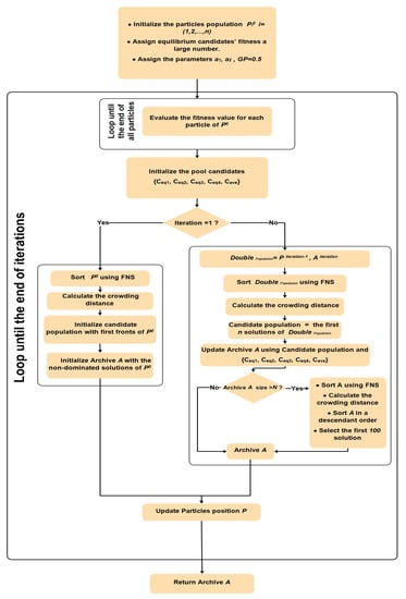
Figure 2.
Flowchart of the proposed GMOEO algorithm.
4. Experimental Results
For evaluating the proposed GMOEO algorithm, several experiments were conducted with 12 different benchmarks, including the test functions of the ZDT series [49] and the DTLZ series [50]. The benchmarking test functions and their properties are reported in Table 1. To further validate our findings, the proposed GMOEO was compared, both qualitatively and quantitatively, with several well-known multi-objective optimization algorithms: namely, the guided multi-objective equilibrium optimizer (with cone--dominance) [45], the multi-objective particle-swarm optimization (MOPSO) [30] method, and the multi-objective grey wolf optimization (MOGWO) [41] method. In all experiments, the number of operations was set at 10, the number of iterations was set at 6000, and the population size was equal to 40. These settings were the same for all algorithms and functions. In our discussion of the results, we refer to GMOEO using an -dominance with -GMOEO, and also to GMOEO using cone--dominance with cone--GMOEO.

Table 1.
Characteristics of the multi-objective test functions.
The comparison was conducted based on three metrics: spacing (SP) [51], maximum spread (MS) [52], and inverted generational distance (IGD) [53].
- SP was used to evaluate the uniformity of the distribution of non-dominated solutions and the diversity of the solutions. The spacing assisted in estimating the distribution of the obtained solution along the Pareto front. SP was defined as follows:wherewhere , with n as the number of solutions obtained in the front, while is the average of all with m as the number of objective functions f;
- MS was used to measure the diagonal length of the hyper-box generated by the extreme values of the objective functions in the non-dominated solution set. MS was defined as follows:where d represents the Euclidean distance between and the maximum value of the ith objective function, and is the minimum value of the ith objective function with M as the number of the objective functions;
- IGD was an inversion of the generational distance metric, which could be computed as the distance between the reference Pareto front and each of the closest non-dominated solutions. Generally, IGD is used as a measure of an algorithm’s convergence. It was formulated as follows:where n represents the number of the true Pareto solution set, while represents the Euclidean distance between the nearest Pareto solution obtained by the algorithm and the true Pareto front: the smaller the IGD and SP, the better the performance. Therefore, these were used to perform the comparison accordingly.
4.1. Results of the ZDT Test Functions
Table 2, Table 3 and Table 4 summarize the statistical results of the metrics IGD, SP, and MS for the ZDT test functions, respectively. Furthermore, to confirm our findings, the qualitative significations of the results are illustrated in Figure 3, Figure 4, Figure 5, Figure 6 and Figure 7. Table 2 lists the statistical results of the IGD metric for the proposed -GMOEO, cone--GMOEO, MOPSO, and MOGWO methods, along with the values for best, worst, average, median, and standard deviations. Overall, in 10 independent operations, the proposed -GMOEO and cone--GMOEO outperformed the well-known MOPSO and MOGWO according to the test functions (ZDT1, ZDT2, ZDT4, and ZDT6). However, -GMOEO provided better results than cone--GMOEO.
Table 2.
Results for the IGD of the ZDT-series test functions.
Table 3.
Results for the SP of the ZDT series test functions.
Table 4.
Results for the MS of the ZDT-series test functions.
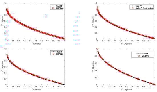
Figure 3.
Pareto front obtained by the -GMOEO dominance, cone--GMOEO dominance, MOPSO, and MOGWO methods for the test function ZDT1.
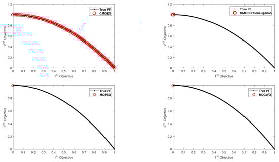
Figure 4.
Pareto front obtained by the -GMOEO dominance, cone--GMOEO dominance, MOPSO, and MOGWO methods for the test function ZDT2.
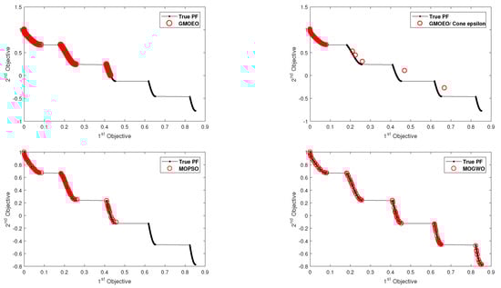
Figure 5.
Pareto front obtained by the -GMOEO dominance, cone--GMOEO dominance, MOPSO, and MOGWO methods for the test function ZDT3.
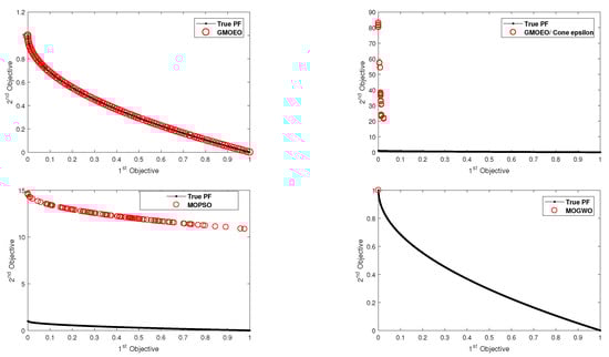
Figure 6.
Pareto front obtained by the -GMOEO dominance, cone--GMOEO dominance, MOPSO, and MOGWO methods for the test function ZDT4.
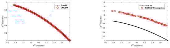
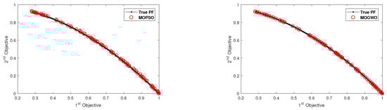
Figure 7.
Pareto front obtained by the -GMOEO dominance, cone--GMOEO dominance, MOPSO, and MOGWO methods for the test function ZDT6.
As for ZDT3 test function, the results proved that MOGWO achieved efficient results as it was able to converge toward all the disconnected fronts, while cone--GMOEO was able to outperform both MOPSO and -GMOEO. Moreover, the reported results related to diversity, which are SP in Table 3 and MS in Table 4, showed that -GMOEO clearly outperformed the other benchmarking algorithms in the bi-objective test function. In addition, the results in Figure 3, Figure 4, Figure 5, Figure 6 and Figure 7 for ZDT1, ZDT2, ZDT4, and ZDT6, respectively, clearly supported our statistical findings and showed that the proposed -GMOEO had better coverage, diversity, and convergence toward the Pareto optimal when compared to the cone--GMOEO, MOPSO, and MOGWO methods. Figure 5 represents the test function ZDT3, as shown in the algorithm, and it shows that MOGWO could perfectly converge toward the disconnected fronts, though cone--GMOEO was also able to converge toward four fronts. Similar to MOPSO, -GMOEO was able to converge toward three fronts. However, -GMOEO showed better coverage. Regarding the IGD value for ZDT3, -GMOEO ranked second after MOGWO. Table 3 shows the statistical results for the SP metric, which proved that the proposed algorithm was highly competitive as -GMOEO had the best results in all the ZDT test functions when compared to the other algorithms. The -GMOEO method had a better distribution over the Pareto front. As shown in Figure 3, Figure 4, Figure 5, Figure 6 and Figure 7, the front generated by -GMOEO was well distributed and extended in all the test functions. The cone--GMOEO method ranked second and was also able to outperform MOPSO and MOGWO in three of the test functions (ZDT1, ZDT2, and ZDT 6). Table 4 shows the results for the MS metric, indicating that -GMOEO was also able to provide efficient results. These outcomes clearly confirmed that our proposed -GMOEO had better diversity in all the test functions. In addition, the cone--GMOEO was also able to compete efficiently in most of the test functions when compared to the other two algorithms (i.e., MOPSO and MOGWO).
To summarize the ZDT test function results, the proposed GMOEO method achieved better outcomes when compared to the other algorithms for IGD, SP, and MS. In particular, -GMOEO was able to outperform the selected benchmarking algorithms, which proved that GMOEO was highly competitive by reaching 100% of the final non-dominated solutions within four different test functions. The metric of convergence IGD was in addition to the diversity, spread, and coverage analysis showing a 100% success rate, and this was the case within all the five different test functions.
4.2. Results of the DTLZ Test Functions
The statistical results for the metrics IGD, SP, and MS for the second test function of DTLZ are summarized in Table 5, Table 6 and Table 7, and the qualitative significance of the results is illustrated in Figure 8, Figure 9, Figure 10, Figure 11, Figure 12, Figure 13 and Figure 14. As shown in Table 5, which represents the IGD metric, the proposed -GMOEO method had the best convergence when compared to the other algorithms. It was able to outperform them in five-in-seven test functions, i.e., DTLZ2 and DTLZ4-7, and it ranked second after MOPSO for the test functions DTLZ1 and DTLZ3. This indicated -GMOEO was able to compete with well-known algorithms in terms of the convergence in challenging test functions, while cone--GMOEO instead ranked last. Figure 8, Figure 9, Figure 10, Figure 11, Figure 12, Figure 13 and Figure 14 plot the IGD metric results, where the -GMOEO method also showed efficient convergence. Furthermore, Table 6 and Table 7 show the diversity metrics of SP and MS, respectively. The presented results in Table 6 and Table 7 indicated that -GMOEO outperformed cone--GMOEO, MOPSO, and MOGWO in five of the test functions (e.g., DTLZ1, DTLZ3, DTLZ5-7) in terms of spacing by obtaining the best average SP value. This confirmed the efficient distribution of the non-dominated solutions over all the true Pareto solutions, as illustrated in Figure 8, Figure 9, Figure 10, Figure 11, Figure 12, Figure 13 and Figure 14. For DTLZ2 and DTLZ4, cone--GMOEO ranked first. For the MS metric, the reported results also showed that -GMOEO provided better diversity than the other benchmarking algorithms. Furthermore, Figure 8, Figure 9, Figure 10, Figure 11, Figure 12, Figure 13 and Figure 14 show the front produced by -GMOEO was well extended and better distributed over the Pareto front, as shown in Figure 11, when compared to the other algorithms. The -GMOEO approach was able to converge and attain efficient distribution and diversity. Moreover, in Figure 14, when compared to the other algorithms, the front generated for DTLZ7 was well distributed and was able to converge and attain all the hyper-planes.
Table 5.
Results for the IGD of the DTLZ-series test functions.
Table 6.
Results for the SP of the DTLZ-series test functions.
Table 7.
Results for the MS of the DTLZ-series test functions.
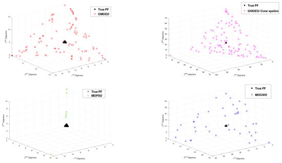
Figure 8.
Pareto front obtained by the -GMOEO dominance, cone--GMOEO dominance, MOPSO, and MOGWO methods for the test function DTLZ1.
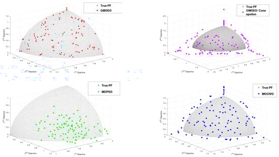
Figure 9.
Pareto front obtained by the -GMOEO dominance, cone--GMOEO dominance, MOPSO, and MOGWO methods for the test function DTLZ2.
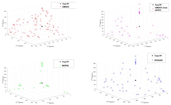
Figure 10.
Pareto front obtained by the -GMOEO dominance, cone--GMOEO dominance, MOPSO, and MOGWO methods for the test function DTLZ3.
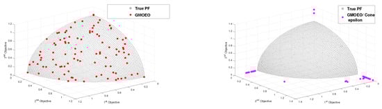
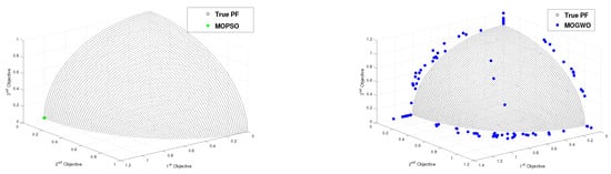
Figure 11.
Pareto front obtained by the -GMOEO dominance, cone--GMOEO dominance, MOPSO, and MOGWO methods for the test function DTLZ4.
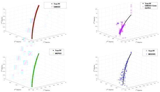
Figure 12.
Pareto front obtained by the -GMOEO dominance, cone--GMOEO dominance, MOPSO, and MOGWO methods for the test function DTLZ5.
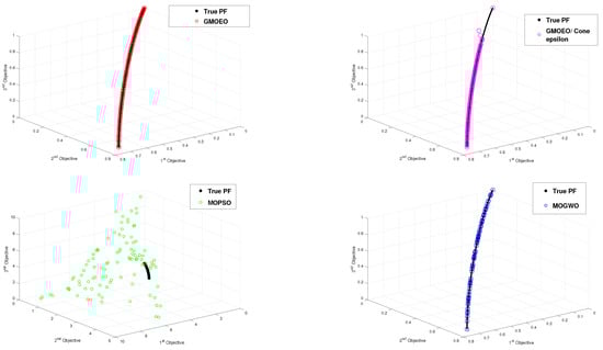
Figure 13.
Pareto front obtained by the -GMOEO dominance, cone--GMOEO dominance, MOPSO, and MOGWO methods for the test function DTLZ6.

Figure 14.
Pareto front obtained by the -GMOEO dominance, cone--GMOEO dominance, MOPSO, and MOGWO methods for the test function DTLZ7.
Therefore, the proposed -GMOEO dominance was very competitive and reliable. It was based on high performance and robustness as indicated by the statistical results for IGD, SP, and MS for the challenging DTLZ test function. In particular, the -GMOEO method was able to outperform the selected benchmarking algorithms by reaching 100% of the final non-dominated solutions within six different test functions and that for the metric of convergence IGD. In addition, the diversity, spread, and coverage analysis showed a 100% success rate and this was the case for all the five different test functions.
As shown in the presented figures, the convergence, coverage, and excellent distribution of the solutions along the Pareto optimal indicated the efficient performance of the proposed -GMOEO method.
To further support the findings and to confirm the performance of the proposed GMOEO algorithm, the Wilcoxon rank-sum test [54] was considered. The analysis was conducted according to the and the level of significance among the compared algorithms. The Wilcoxon rank-sum test would assist in establishing the significant differences according to the null-hypothesis (): If , then no significant difference between the results of the algorithms could be found. However, if , then a significant difference was found ().
Therefore, we evaluated the of the IGD and SP metrics that were obtained after ten operations by comparing each pair of -GMOEO and cone--GMOEO, and MOPSO and MOGWO for each test function with a significance of . According to the results for the IGD metric shown in Table 8, the -GMOEO outperformed all the benchmarking algorithms in all the test functions, with both bi- and tri-objectives. As shown in Table 8, the indicated that the hypothesis was confirmed. Furthermore, the results showed that the proposed GMOEO was able to converge toward the Pareto optimal more efficiently than the other algorithms, including cone--GMOEO. According to the results of the SP metric shown in Table 9, the -GMOEO method outperformed all other algorithms in of the test functions.
Table 8.
The results for the Wilcoxon rank-sum test of the IGD metric.
Table 9.
The for the Wilcoxon rank-sum test of the SP metric.
Therefore, -GMOEO has better diversity and spread. In summary, the results of the Wilcoxon rank-sum test proved that -GMOEO was highly competitive when compared to existing algorithms as it did the best 100% of the time. In addition, the performance of -GMOEO was capable of nearly reaching the Pareto front reliably. Finally, we confirmed that the archive population and update strategies were effective for increasing the reliability of GMOEO, along with the application of the crowding distance and FNS methods. Furthermore, -dominance was a better option for updating the archive when compared to cone--dominance, even though the latter had outperformed some of the benchmarking algorithms. However, it was not as effective as -dominance.
5. Conclusions
In this study, we proposed a guided multi-objective equilibrium optimizer (GMOEO) to solve MOPs. The GMOEO algorithm was developed by extending the equilibrium optimizer via an external archive to guide the population toward the Pareto optimal. Furthermore, fast non-dominated sorting and crowding distance methods were introduced into the GMOEO algorithm in order to control the quality of the solutions and to ensure the diversity and convergence factors. More importantly, we explored two relations, i.e., -dominance and cone--dominance, for the purposes of managing the archive population’s best non-dominated solutions. In addition, a candidate population was proposed to aid in updating the archive. A benchmarking study was conducted with the well-known MOPSO and MOGWO algorithms on 12 widely used benchmark functions. The obtained results indicated that the proposed GMOEO is a powerful and competitive tool with high efficacy. It was able to outperform other algorithms. Moreover, according to the statistical and graphical results for this algorithm, we were able to realize -dominance as a better strategy for updating the archive when compared to the cone--dominance. Finally, the proposed GMOEO was a reliable tool for solving multi-objective optimization problems. GMOEO could also be a efficient tool for solving several engineering optimization problems, such as the design of pressure vessels, vibrating platform, and gear trains, as well as other problems—the results showed GMOEO’s potential for such applications.
Author Contributions
Conceptualization, A.B. (Abderraouf Bouziane) and A.B. (Adel Binbusayyis); methodology, N.E.C. and A.A. (Abdelouahab Attia); software, N.E.C.; validation, M.H.; formal analysis, M.H., A.A. (Abdelouahab Attia), and A.A. (Abed Alanazi); writing—original draft preparation, N.E.C. and A.A. (Abdelouahab Attia); writing—review and editing, M.H., A.A. (Abed Alanazi), and A.B. (Adel Binbusayyis); project administration, A.B. (Adel Binbusayyis) and A.A. (Abdelouahab Attia); funding acquisition, M.H., A.A. (Abed Alanazi) and A.B. (Adel Binbusayyis). All authors have read and agreed to the published version of the manuscript.
Funding
Funding was received from Prince Sattam bin Abdulaziz University (project number (PSAU/2023/R/1444)).
Data Availability Statement
Not applicable.
Acknowledgments
This study was supported via funding from Prince Sattam bin Abdulaziz University (project number (PSAU/2023/R/1444)).
Conflicts of Interest
The authors declare no conflict of interests.
References
- Dahou, A.; Chelloug, S.A.; Alduailij, M.; Elaziz, M.A. Improved Feature Selection Based on Chaos Game Optimization for Social Internet of Things with a Novel Deep Learning Model. Mathematics 2023, 11, 1032. [Google Scholar] [CrossRef]
- Mohamed, A.A.; Abdellatif, A.D.; Alburaikan, A.; Khalifa, H.A.E.W.; Elaziz, M.A.; Abualigah, L.; AbdelMouty, A.M. A novel hybrid arithmetic optimization algorithm and salp swarm algorithm for data placement in cloud computing. Soft Comput. 2023, 27, 5769–5780. [Google Scholar] [CrossRef]
- Vijaya Bhaskar, K.; Ramesh, S.; Karunanithi, K.; Raja, S. Multi Objective Optimal Power Flow Solutions using Improved Multi Objective Mayfly Algorithm (IMOMA). J. Circuits Syst. Comput. 2023. [Google Scholar] [CrossRef]
- Perera, J.; Liu, S.H.; Mernik, M.; Črepinšek, M.; Ravber, M. A Graph Pointer Network-Based Multi-Objective Deep Reinforcement Learning Algorithm for Solving the Traveling Salesman Problem. Mathematics 2023, 11, 437. [Google Scholar] [CrossRef]
- Zhang, Z.; Gao, S.; Lei, Z.; Xiong, R.; Cheng, J. Pareto Dominance Archive and Coordinated Selection Strategy-Based Many-Objective Optimizer for Protein Structure Prediction. IEEE/ACM Trans. Comput. Biol. Bioinform. 2023, 20, 2328–2340. [Google Scholar] [CrossRef]
- De, S.; Dey, S.; Bhattacharyya, S. Recent Advances in Hybrid Metaheuristics for Data Clustering; John Wiley & Sons: Hoboken, NJ, USA, 2020. [Google Scholar]
- Bhattacharyya, S. Hybrid Computational Intelligent Systems: Modeling, Simulation and Optimization; CRC Press: Boca Raton, FL, USA, 2023. [Google Scholar]
- Bhattacharyya, S.; Banerjee, J.S.; De, D. Confluence of Artificial Intelligence and Robotic Process Automation; Springer: Berlin/Heidelberg, Germany, 2023. [Google Scholar]
- Mahmoodabadi, M. An optimal robust fuzzy adaptive integral sliding mode controller based upon a multi-objective grey wolf optimization algorithm for a nonlinear uncertain chaotic system. Chaos Solitons Fractals 2023, 167, 113092. [Google Scholar] [CrossRef]
- Chalabi, N.E.; Attia, A.; Bouziane, A.; Hassaballah, M. An improved marine predator algorithm based on Epsilon dominance and Pareto archive for multi-objective optimization. Eng. Appl. Artif. Intell. 2023, 119, 105718. [Google Scholar] [CrossRef]
- Feng, X.; Pan, A.; Ren, Z.; Fan, Z. Hybrid driven strategy for constrained evolutionary multi-objective optimization. Inf. Sci. 2022, 585, 344–365. [Google Scholar] [CrossRef]
- Houssein, E.H.; Saad, M.R.; Hashim, F.A.; Shaban, H.; Hassaballah, M. Lévy flight distribution: A new metaheuristic algorithm for solving engineering optimization problems. Eng. Appl. Artif. Intell. 2020, 94, 103731. [Google Scholar] [CrossRef]
- Deb, K.; Pratap, A.; Agarwal, S.; Meyarivan, T. A fast and elitist multiobjective genetic algorithm: NSGA-II. IEEE Trans. Evol. Comput. 2002, 6, 182–197. [Google Scholar] [CrossRef]
- Deb, K.; Jain, H. An evolutionary many-objective optimization algorithm using reference-point-based nondominated sorting approach, part I: Solving problems with box constraints. IEEE Trans. Evol. Comput. 2013, 18, 577–601. [Google Scholar] [CrossRef]
- Knowles, J.D.; Corne, D.W. M-PAES: A memetic algorithm for multiobjective optimization. In Proceedings of the Congress on Evolutionary Computation CEC00 (Cat. No. 00TH8512), La Jolla, CA, USA, 16–19 July 2000; Volume 1, pp. 325–332. [Google Scholar]
- Zitzler, E.; Laumanns, M.; Thiele, L. SPEA2: Improving the strength Pareto evolutionary algorithm. TIK-Report 2001, 103. [Google Scholar] [CrossRef]
- Daliri, A.; Asghari, A.; Azgomi, H.; Alimoradi, M. The water optimization algorithm: A novel metaheuristic for solving optimization problems. Appl. Intell. 2022, 52, 17990–18029. [Google Scholar] [CrossRef]
- Qin, S.; Pi, D.; Shao, Z.; Xu, Y.; Chen, Y. Reliability-Aware Multi-Objective Memetic Algorithm for Workflow Scheduling Problem in Multi-Cloud System. IEEE Trans. Parallel Distrib. Syst. 2023, 34, 1343–1361. [Google Scholar] [CrossRef]
- Abd Elaziz, M.; Abualigah, L.; Issa, M.; Abd El-Latif, A.A. Optimal parameters extracting of fuel cell based on Gorilla Troops Optimizer. Fuel 2023, 332, 126162. [Google Scholar] [CrossRef]
- Dutta, T.; Bhattacharyya, S.; Panigrahi, B.K. Multilevel Quantum Evolutionary Butterfly Optimization Algorithm for Automatic Clustering of Hyperspectral Images. In Proceedings of the 3rd International Conference on Artificial Intelligence and Computer Vision, Taiyuan, China, 26–28 May 2023; pp. 524–534. [Google Scholar]
- Zhang, Q.; Li, H. MOEA/D: A multiobjective evolutionary algorithm based on decomposition. IEEE Trans. Evol. Comput. 2007, 11, 712–731. [Google Scholar] [CrossRef]
- Deb, K.; Mohan, M.; Mishra, S. Evaluating the ε-domination based multi-objective evolutionary algorithm for a quick computation of Pareto-optimal solutions. Evol. Comput. 2005, 13, 501–525. [Google Scholar] [CrossRef]
- Ma, X.; Qi, Y.; Li, L.; Liu, F.; Jiao, L.; Wu, J. MOEA/D with uniform decomposition measurement for many-objective problems. Soft Comput. 2014, 18, 2541–2564. [Google Scholar] [CrossRef]
- Tan, Y.Y.; Jiao, Y.C.; Li, H.; Wang, X.K. MOEA/D-SQA: A multi-objective memetic algorithm based on decomposition. Eng. Optim. 2012, 44, 1095–1115. [Google Scholar] [CrossRef]
- Qiao, K.; Liang, J.; Yu, K.; Wang, M.; Qu, B.; Yue, C.; Guo, Y. A Self-Adaptive Evolutionary Multi-Task Based Constrained Multi-Objective Evolutionary Algorithm. IEEE Trans. Emerg. Top. Comput. Intell. 2023. [Google Scholar] [CrossRef]
- Wang, Q.; Gu, Q.; Chen, L.; Guo, Y.; Xiong, N. A MOEA/D with global and local cooperative optimization for complicated bi-objective optimization problems. Appl. Comput. 2023, 137, 110162. [Google Scholar] [CrossRef]
- Eberhart, R.; Kennedy, J. A new optimizer using particle swarm theory. In Proceedings of the Sixth International Symposium on Micro Machine and Human Science, Nagoya, Japan, 4–6 October 1995; pp. 39–43. [Google Scholar]
- Rabbani, M.; Oladzad-Abbasabady, N.; Akbarian-Saravi, N. Ambulance routing in disaster response considering variable patient condition: NSGA-II and MOPSO algorithms. J. Ind. Manag. Optim. 2022, 18, 1035–1062. [Google Scholar] [CrossRef]
- Ray, T.; Liew, K. A swarm metaphor for multiobjective design optimization. Eng. Optim. 2002, 34, 141–153. [Google Scholar] [CrossRef]
- Coello, C.A.C.; Pulido, G.T.; Lechuga, M.S. Handling multiple objectives with particle swarm optimization. IEEE Trans. Evol. Comput. 2004, 8, 256–279. [Google Scholar] [CrossRef]
- Dorigo, M.; Di Caro, G. Ant colony optimization: A new meta-heuristic. In Proceedings of the Congress on Evolutionary Computation-CEC99 (Cat. No. 99TH8406), Washington, DC, USA, 6–9 July 1999; Volume 2, pp. 1470–1477. [Google Scholar]
- Kaveh, M.; Mesgari, M.S.; Saeidian, B. Orchard Algorithm (OA): A new meta-heuristic algorithm for solving discrete and continuous optimization problems. Math. Comput. Simul. 2023, 208, 95–135. [Google Scholar] [CrossRef]
- Rada-Vilela, J.; Chica, M.; Cordón, Ó.; Damas, S. A comparative study of multi-objective ant colony optimization algorithms for the time and space assembly line balancing problem. Appl. Soft Comput. 2013, 13, 4370–4382. [Google Scholar] [CrossRef]
- Pu, X.; Song, X.; Tan, L.; Zhang, Y. Improved ant colony algorithm in path planning of a single robot and multi-robots with multi-objective. Evol. Intell. 2023. [Google Scholar] [CrossRef]
- Zhang, D.; Luo, R.; Yin, Y.b.; Zou, S.l. Multi-objective path planning for mobile robot in nuclear accident environment based on improved ant colony optimization with modified A. Nucl. Eng. Technol. 2023, 55, 1838–1854. [Google Scholar] [CrossRef]
- Flor-Sánchez, C.O.; Reséndiz-Flores, E.O.; García-Calvillo, I.D. Kernel-based hybrid multi-objective optimization algorithm (KHMO). Inf. Sci. 2023, 624, 416–434. [Google Scholar] [CrossRef]
- Singh, P.; Muchahari, M.K. Solving multi-objective optimization problem of convolutional neural network using fast forward quantum optimization algorithm: Application in digital image classification. Adv. Eng. Softw. 2023, 176, 103370. [Google Scholar] [CrossRef]
- Chu, S.C.; Tsai, P.W. Computational intelligence based on the behavior of cats. Int. J. Innov. Comput. Inf. Control 2007, 3, 163–173. [Google Scholar]
- Pradhan, P.M.; Panda, G. Solving multiobjective problems using cat swarm optimization. Expert Syst.Appl. 2012, 39, 2956–2964. [Google Scholar] [CrossRef]
- Mirjalili, S.; Mirjalili, S.M.; Lewis, A. Grey wolf optimizer. Adv. Eng. Softw. 2014, 69, 46–61. [Google Scholar] [CrossRef]
- Mirjalili, S.; Saremi, S.; Mirjalili, S.M.; Coelho, L.d.S. Multi-objective grey wolf optimizer: A novel algorithm for multi-criterion optimization. Expert Syst. Appl. 2016, 47, 106–119. [Google Scholar] [CrossRef]
- Zouache, D.; Abdelaziz, F.B.; Lefkir, M.; Chalabi, N.E.H. Guided Moth–Flame optimiser for multi-objective optimization problems. Ann. Oper. Res. 2021, 296, 877–899. [Google Scholar] [CrossRef]
- Mirjalili, S. Moth-flame optimization algorithm: A novel nature-inspired heuristic paradigm. Knowl.-Based Syst. 2015, 89, 228–249. [Google Scholar] [CrossRef]
- Houssein, E.H.; Çelik, E.; Mahdy, M.A.; Ghoniem, R.M. Self-adaptive Equilibrium Optimizer for solving global, combinatorial, engineering, and Multi-Objective problems. Expert Syst. Appl. 2022, 195, 116552. [Google Scholar] [CrossRef]
- Faramarzi, A.; Heidarinejad, M.; Stephens, B.; Mirjalili, S. Equilibrium optimizer: A novel optimization algorithm. Knowl.-Based Syst. 2020, 191, 105190. [Google Scholar] [CrossRef]
- Laumanns, M.; Thiele, L.; Deb, K.; Zitzler, E. Combining convergence and diversity in evolutionary multiobjective optimization. Evol. Comput. 2002, 10, 263–282. [Google Scholar] [CrossRef]
- Batista, L.S.; Campelo, F.; Guimaraes, F.G.; Ramírez, J.A. Pareto cone ε-dominance: Improving convergence and diversity in multiobjective evolutionary algorithms. In Proceedings of the International Conference on Evolutionary Multi-Criterion Optimization, Ouro Preto, Brazil, 5–8 April 2011; pp. 76–90. [Google Scholar]
- Ikeda, K.; Kita, H.; Kobayashi, S. Failure of Pareto-based MOEAs: Does non-dominated really mean near to optimal? In Proceedings of the Congress on Evolutionary Computation (Cat. No. 01TH8546), Seoul, Republic of Korea, 27–30 May 2001; Volume 2, pp. 957–962. [Google Scholar]
- Zitzler, E.; Deb, K.; Thiele, L. Comparison of multiobjective evolutionary algorithms: Empirical results. Evol. Comput. 2000, 8, 173–195. [Google Scholar] [CrossRef]
- Deb, K.; Thiele, L.; Laumanns, M.; Zitzler, E. Scalable multi-objective optimization test problems. In Proceedings of the Congress on Evolutionary Computation (Cat. No. 02TH8600), Honolulu, HI, USA, 12–17 May 2002; Volume 1, pp. 825–830. [Google Scholar]
- Schott, J.R. Fault Tolerant Design Using Single and Multicriteria Genetic Algorithm Optimization. Ph.D Thesis, Massachusetts Institute of Technology, Cambridge, MA, USA, 1995. [Google Scholar]
- Zitzler, E.; Thiele, L. Multiobjective optimization using evolutionary algorithms—A comparative case study. In Proceedings of the International Conference on Parallel Problem Solving From Nature, Amsterdam, The Netherlands, 27–30 September 1998; pp. 292–301. [Google Scholar]
- Van Veldhuizen, D.A.; Lamont, G.B. Multiobjective evolutionary algorithms: Analyzing the state-of-the-art. Evol. Comput. 2000, 8, 125–147. [Google Scholar] [CrossRef] [PubMed]
- Derrac, J.; García, S.; Molina, D.; Herrera, F. A practical tutorial on the use of nonparametric statistical tests as a methodology for comparing evolutionary and swarm intelligence algorithms. Swarm Evol. Comput. 2011, 1, 3–18. [Google Scholar] [CrossRef]
Disclaimer/Publisher’s Note: The statements, opinions and data contained in all publications are solely those of the individual author(s) and contributor(s) and not of MDPI and/or the editor(s). MDPI and/or the editor(s) disclaim responsibility for any injury to people or property resulting from any ideas, methods, instructions or products referred to in the content. |
© 2023 by the authors. Licensee MDPI, Basel, Switzerland. This article is an open access article distributed under the terms and conditions of the Creative Commons Attribution (CC BY) license (https://creativecommons.org/licenses/by/4.0/).