Gearbox Fault Diagnosis Based on Multi-Sensor Deep Spatiotemporal Feature Representation

Abstract

The vibration signal acquired by a single sensor contains limited information and is easily interfered by noise signals, resulting in the inability to fully express the operating characteristics and state of a gearbox. To address this problem, our study proposes a gearbox fault diagnosis method based on multi-sensor deep spatiotemporal feature representation. This method utilizes two vibration sensors to obtain the vibration information of the gearbox. A fault diagnosis model (PCNN–GRU) combined with a parallel convolutional neural network (PCNN) and gated recurrent unit (GRU) was used to fuse the gearbox vibration information. The parallel convolutional neural network was used to extract the spatial information of the vibration signals collected by different position sensors, and the timing information was mined through the gated recurrent unit. The deep spatiotemporal features that fuse the multi-sensor spatial and temporal information were composed. The collected multi-sensor vibration signals were directly input into the PCNN–GRU model, and an end-to-end intelligent diagnosis of the gearbox faults was realized. Finally, through experimental verification, the accuracy rate of this model can reach up to 99.92%. Compared with other models, this model has a higher diagnostic accuracy and stability.

1. Introduction

The gearbox is a common rotating mechanical device used to transmit power, and it is widely used in various fields. Once the gear box breaks down, it will directly affect industrial production and daily life [1,2]. Severe cases may even cause personal injury and serious economic losses [3]. Therefore, carrying out a fault diagnosis on—as well as the timely detection and troubleshooting of—a gearbox and its key components plays a key role in ensuring the healthy operation of mechanical equipment and reducing equipment maintenance costs. The gearbox has a complex structure, and the interaction between its various parts during operation is accompanied by the interference of environmental noise [4]. The means with which to extract useful information from vibration signals containing complex information and interference components, along with realizing the intelligent diagnosis of gearboxes and its key component failures have particularly important practical significance for the normal operation of mechanical equipment and the improvement of production efficiencies.

Methods for the fault diagnosis of gearboxes can generally be divided into three categories: signal-processing-based methods [5], traditional machine learning-based methods [6], and deep learning-based methods [7]. The signal-processing method mainly completes the fault diagnosis of the gearbox by analyzing the acquired vibration signal and extracting the characteristic information that can reflect the health condition [8]. The methods based on signal processing are usually diagnosed and analyzed from the time domain, frequency domain, and time–frequency domain. Although the methods based on signal processing have made some achievements in the fault diagnosis of rotating equipment such as gearboxes, they require strong manual experience and theoretical knowledge reserves in the process of diagnosis [9,10]. Especially in the face of massive data collection in engineering, it is difficult to realize automatic and intelligent fault diagnosis.

The fault diagnosis method based on traditional machine learning methods mainly extracts useful feature indexes that can represent vibration signals through signal processing methods [11]. Additionally, a shallow machine learning method to perform pattern recognition and to complete the intelligent diagnosis of gearbox faults can be conducted [12]. The commonly used shallow machine learning methods mainly include the BP neural network [13], the support vector machine (SVM) [14], the extreme learning machine (ELM) [15], and other models. Although the traditional machine learning algorithm can realize the intelligent diagnosis of faults, it improves the efficiency and accuracy of a fault diagnosis to a certain extent [16]. However, there is still the limitation that the manual feature extraction of vibration signals is required, and existing feature-extraction methods still rely on signal-processing methods. At the same time, whether the feature extraction is good or not will have a direct impact on the subsequent pattern recognition and classification accuracy [17,18].

The concept of deep learning was first proposed by scholars such as Hinton [19], and it has been widely used in image processing and in other directions. In recent years, more and more scholars have applied deep learning models to conduct a fault diagnosis of mechanical equipment. Compared with the traditional fault diagnosis method of the machine learning model, the fault diagnosis method based on a deep learning model does not need manual feature extraction. Using the stacked multi-layer nonlinear layers in the deep learning model can automatically complete the mining of latent features inside the signal [20]. The dependence on signal-processing-based feature-extraction methods and the influence of human experience on feature extraction are reduced. The generalization performance and adaptability of the fault diagnosis method are improved [21]. Huang et al. [22] input the vibration signal of the gearbox that was decomposed by the wavelet packet into the multi-scale CNN and realized the effective classification of the faults. This method combines the multi-scale characteristics of WPD and the powerful classification ability of CNN, without the complicated manual feature-extraction steps adopted. This end-to-end intelligent fault diagnosis is worth learning. Jin et al. [23] proposed a light neural network based on CNN that can realize the effective diagnosis of rotating machinery faults, such as gearboxes, with fewer parameters, and it maintains a good diagnostic performance under different working conditions. However, the scale of this light neural network is small and the number of parameters is limited, which is prone to overfitting problems in the training process. Yin et al. [24] used LSTM with cosine loss to improve the classification ability of wind turbine gearbox faults. By introducing memory units and gating mechanisms, LSTM can effectively capture and maintain long-term dependencies of information, making it perform well in processing long sequence data. Miao et al. [25] used GRU for the real-time status monitoring of planetary gearboxes and introduced dropout technology to reduce the requirements for training data, which has good real-time diagnostic capabilities. GRU has a more compact structure than LSTM, reducing the number of required parameters. Thus, the GRU model is relatively light and is easier to train and compute. If CNN and GRU can be combined to obtain the deep spatiotemporal features of spatial information and temporal information, good results may be obtained.

With the continuous improvement of sensor technology, sensors are used to obtain various signals that can effectively characterize the operating status of equipment. Additionally, the use of the acquired signal to analyze the health status of mechanical equipment has been widely studied by, and has been of interest for, many scholars in recent years [26]. In fault diagnoses, signals such as vibration, acoustic emission, oil, and temperature are commonly used for analysis. Compared with other signals, vibration signal detection technology is more mature and is easy to operate; it also contains a wealth of useful information, such that it is often used to analyze the health status of rotating machinery. At the same time, thanks to the advancement of artificial intelligence technology, fault diagnosis methods have also developed rapidly. In particular, the advancement of machine learning and deep learning methods has gradually reduced the dependence on expert experience and human judgment for fault diagnoses [27]. Intelligent fault diagnosis has gradually become an important direction for gearbox fault diagnosis.

In summary, this paper proposes a gearbox fault diagnosis method based on multi-sensor deep spatiotemporal feature representation. The contributions of this paper are as follows:

(1)

The vibration signal obtained by a single sensor is susceptible to noise interference and cannot effectively characterize the operating state and fault characteristics of the gearbox. At the same time, it is also necessary to obtain a more effective and stable gearbox fault diagnosis model. A fault diagnosis model based on the PCNN–GRU fusion of multi-sensor information is proposed.

(2)

On the basis of CNN–GRU, a parallel CNN combined with the GRU fault diagnosis model is proposed to fuse the vibration signal information acquired by the multiple sensors. Additionally, SoftMax was used to identify and complete the intelligent diagnosis of gearbox “end” to “end”.

(3)

A fault diagnosis experiment platform was designed and built, and the validity and stability of the model proposed in this paper were verified by comparing it against other related models.

The remainder of this paper is organized as follows: Section 2 introduces the relevant background of this paper, including the CNN, GRU, and multi-sensor information fusion technology; Section 3 introduces the construction of the relevant fault diagnosis model in this paper; Section 4 introduces the construction of the gearbox fault diagnosis experiment platform and the data collection and division; Section 5 is the experimental analysis and verification section; and, lastly, Section 6 contains the conclusion of this paper.

2. Principle Introduction

2.1. CNN

Convolutional neural networks (CNNs) are feedforward neural networks with a deep structure. They have been widely used in the field of fault diagnosis, and their main structures include convolutional layers, pooling layers, and fully connected layers [28]. CNNs extract features through multiple-stacked convolutional layers and pooling layers, and they complete the output of features through fully connected layers [29].

2.1.1. Convolutional Layer

The convolutional layer is the core component of CNNs and is the basic unit of a CNN. The convolutional layer has the characteristics of weight sharing, which can effectively reduce the parameters of the deep network during the training process. It reduces the complexity of the model and improves the training speed [30]. In CNN, each convolutional layer contains multiple convolutional kernels, and the optimal parameters of these convolutional kernels are obtained through the backpropagation algorithm. At the same time, the convolution kernel is used as a filter to effectively extract the key features of the input information. The inner product operation is performed between the input information and the convolution kernel [31]. Usually, after the convolution operation between the input data and the convolution kernel, a bias item needs to be added to the result to obtain the final output result. Its calculation formula is shown in Formula (1):

$$x_j^l=f\left({\displaystyle \sum _{i\in M_j}^n{x}_i^{l-1}}\ast k_{i,j}^l+b_j^l\right)$$

(1)

In Formula (1), $l$ is the number of convolutional layers and $x_j^l$ is the output result of the $l$-th convolutional layer. $x_i^{l-1}$ is the input information of the $l$-th convolutional layer. $k_{i,j}^l$ is the convolution kernel of the l-th convolutional layer and $b_j^l$ is the bias item. $f(•)$ is the activation function. $M_j$ denotes input data.

In the calculation process of the convolutional layer, the size of the output information is mainly expressed by Formula (2):

$$O_1=\frac{H_1-W_1+2\times P}{S}+1$$

(2)

In Formula (2), $O_1$ is the size of the output information. $H_1$ is the size of the input information. $W_1$ is the size of the convolution kernel. $P$ is the zero complement operation in the convolution process. $S$ is the step size of the convolution operation.

2.1.2. Pooling Layer

In CNNs, a pooling layer is usually added after the convolutional layer. The pooling layer can select features and can effectively reduce the output feature dimension. While retaining useful features, the calculation amount and parameters of the network are effectively reduced, and the calculation efficiency is improved [32]. Therefore, this is also called the downsampling layer, and it can also prevent overfitting from occurring. The pooling layer is mainly divided into two types: average pooling and maximum pooling. Average pooling averages the values within a range. Max pooling is to keep the maximum value in the range [33]. Formula (3) is the calculation formula for the output size of the pooling layer:

$$O_2=\frac{H_2-W_2}{S}+1$$

(3)

In Formula (3), $O_2$ is the output size of the pooling layer; $H_2$ is the size of the input information; and $W_2$ is the size of the pooling window.

2.1.3. Activation Function

In practical problems, most of the problems are nonlinear problems. The activation function can map the output linear results to a nonlinear space such that the neural network can learn and train nonlinear models as well as improve the ability of the neural network to deal with nonlinear problems. Sigmoid, Tanh, and ReLU are commonly used activation functions [34].

2.1.4. Fully Connected Layer

The role of the fully connected layer is that it is mainly used for classification. The fully connected layer is often set after multi-layer convolution and pooling. It can effectively integrate the feature information obtained by multi-layer convolution kernel pooling. The SoftMax logistic regression function is often used for classification. The SoftMax function can map the input to a real number between 0 and 1. All neurons in the previous layer of the fully connected layer are connected to neurons in the fully connected layer [35]. Therefore, the parameters and calculation amount in this layer are often relatively large. The calculation expression for the forward propagation of the fully connected layer is shown in Formula (4):

$$Z_j^l=f\left({\displaystyle \sum _{k=i}^n{w}_i^l{x}_i^l+b_j^l}\right)$$

(4)

In Formula (4), $i$ represents the number and $l$ represents the number of layers. $w_i^l$ represents the connection weight between the $i$-th neuron of the $l$-th layer and the $i$-th neuron of the neurons of the previous layer. $b_j^l$ is the bias item of the $j$-th neuron in the $l$-th layer. $f(•)$ is the activation function.

2.2. GRU

A gated recurrent unit (GRU) is a simplified form of a long short-term memory (LSTM) model. Compared with LSTM, GRU has a simpler structure that can efficiently mine the inner connection and long-term information of a time series [36]. Compared with the traditional RNN, GRU not only has smaller training parameters, but it can also effectively solve the problem of gradient disappearance. Structurally, only two gates are included in the GRU—the update gate and the reset gate—both of which belong to the gating mechanism [37]. The GRU gating mechanism is crucial for the correct operation of the model. Specifically, resetting the part and previous hidden states play an important role in determining candidate hidden states. The structure of the GRU in this study is shown in Figure 1:

In a GRU, the reset gate helps the model decide how much of the previous hidden state should be forgotten or reset. It determines which parts of the previous hidden state are relevant to the current step of the model. The reset gate is usually a sigmoid function that takes as input the concatenation of the current input and the previous hidden state. Candidate hidden states are intermediate states computed using the reset gate and the current input. It is combined with the previous hidden state, considering the update gate, to produce the final hidden state of the GRU.

The states of the update gate $z_t$ and the reset gate $r_t$ are obtained by the output state $h_{t-1}$ at the previous moment and the input data $x_t$ at this time. Among them, the update gate is used to evaluate the importance of the information at the last moment to determine the size of the information transmitted to the current hidden layer. Its calculation formula is shown in Formula (5):

$$z_t=\sigma \left(w_z{x}_t+w_z{h}_{t-1}+b_z\right)$$

(5)

In Formula (5), $\sigma$ represents the sigmoid function, such that the result is distributed between 0 and 1. Thus, 1 means it retains information completely, and 0 means it ignores information completely. $w_z$ and $w_z$ are denoted as weights and biases, respectively. The reset gate is used to determine the information size of the previous moment that needs to be ignored. Its calculation formula is shown in Formula (6):

$$r_t=\sigma \left(w_r{x}_t+w_r{h}_{t-1}+b_r\right)$$

(6)

In Formula (6), $\sigma$ represents the sigmoid function; $w_r$ and $b_r$ represent the weight and bias, respectively. The information ${\tilde{h}}_t$ at the current moment can be obtained by Formula (7):

$${\tilde{h}}_t=\tanh \left(w_h{x}_t+r_t\otimes w_h{h}_{t-1}\right)$$

(7)

In Formula (7), $\otimes$ is the Hadamard product. Tanh is the hyperbolic tangent function used to distribute the result between −1 and 1. $w_h$ is the weight. Then, the final output result Ht is obtained according to Formula (8):

$$h_t=z_t\otimes h_{t-1}+\left(1-z_t\right)\otimes {\tilde{h}}_t$$

(8)

where $h_t$ is the final output result, $z_t$ is the update gate, and ${\tilde{h}}_t$ is obtained by Formula (7).

2.3. Multi-Sensor Information Fusion

Multi-sensor information fusion can effectively reduce the information loss caused by a single sensor, and it can improve the accuracy and stability of fault diagnosis [38]. The method of multi-sensor information fusion is mainly divided into three levels: the data level, feature level, and decision level [39].

2.3.1. Fusion at the Data Level

Fusion at the data level refers to the direct fusion of the information acquired by multiple sensors; then, feature-extraction and pattern-recognition operations on the fused information are performed. They belong to the most primitive of information fusion approaches.

2.3.2. Fusion at the Feature Level

The information is fused at the feature level. That is, the feature-extraction operation is performed separately on the information obtained by multiple sensors, and the features representing different sensor information are fused. Finally, a pattern recognition method is used to recognize the fusion features.

2.3.3. Fusion at the Decision-Making Level

Fusion at the decision-making level is a type of advanced fusion method. After the information of different sensors is preprocessed, separate decisions are made on the tested equipment. Finally, different decisions are fused to obtain a final decision with overall consistency.

The advantages and disadvantages of the different levels of the fusion methods are shown in

Table 1. Advantages and disadvantages of the different integration methods.

Information Fusion Method	Advantages	Disadvantages
Data level	Less information loss, higher fusion accuracy	The amount of calculation is too large, and the information needs to come from the same type of sensor
Feature level	Can effectively compress and extract information	Recognition accuracy depends on whether the proposed features are valid
Decision-making level	Has strong anti-interference ability, no requirement for sensor type	Large amount of information loss and poor accuracy

:

Due to the information fusion at the feature level, different sensor information can be effectively compressed. Therefore, this paper proposes a fault diagnosis model combining a parallel convolutional neural network and gated recurrent unit (PCNN–GRU) to automatically mine the intrinsic characteristics of vibration signals acquired by the sensors at different positions; in addition, complete information fusion is used at the feature level.

3. Fault Diagnosis Model Construction

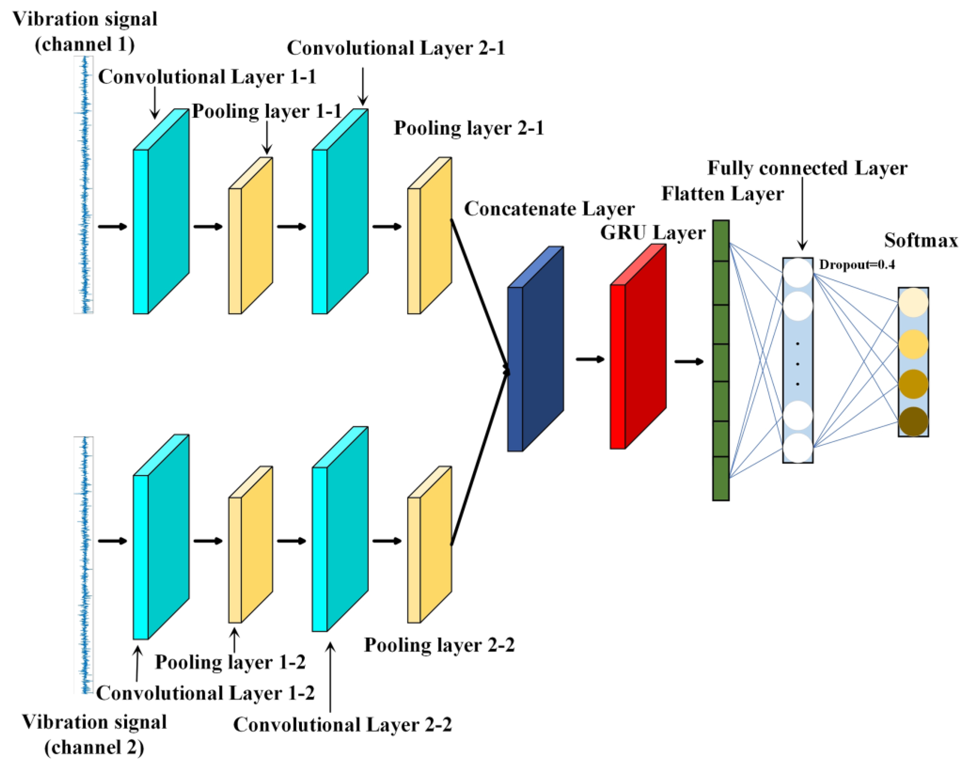
According to the complexity of the network model and the scale of the data obtained from the designed fault diagnosis experiment, as well as multiple experiments to adjust and optimize the model parameters, a fault diagnosis model is constructed. The structure of the fault diagnosis model proposed in this paper based on PCNN–GRU fusion of multi-sensor information is shown in Figure 2. The model structure parameters are shown in

Table 2. The parameters of each layer of the PCNN–GRU model.

Network Layer	Number of Convolution Kernels	Convolution Kernel Size	Step Length	Activation Function	Output Size
Convolutional layer 1–1	32	64	8	ReLU	256 × 32
Pooling layer 1–1	32	4	1	—	64 × 32
Convolutional layer 2–1	64	5	1	ReLU	64 × 64
Pooling layer 2–1	64	2	1	—	32 × 64
Convolutional layer 1–2	32	64	8	ReLU	256 × 32
Pooling layer 1–2	32	4	1	—	64 × 32
Convolutional layer 2–2	64	5	1	ReLU	64 × 64
Pooling layer 2–2	64	2	1	—	32 × 64
Fusion layer	—	—	—	—	32 × 128
GRU layer	16	—	—	Tanh	32 × 16
Fully connected layer	32	—	—	Tanh	32
SoftMax	4	—	—	SoftMax	4

.

From Figure 2 and Table 2, it can be seen that the model mainly consists of two parallel convolutional neural network layers, a fusion layer, a gated loop unit layer, and two fully connected layers (the last layer is the SoftMax layer for the final classification). Parallel convolutional neural networks are composed of two one-dimensional convolutional layers and two one-dimensional pooling layers. Additionally, the model structure parameters of the upper and lower channels are set as the same. The number of convolutional kernels, the kernel size, and the stride of convolutional layer 1–1 and convolutional layer 1–2 were all set to 32, 64, and 8, respectively. The number of convolution kernels, the kernel size, and the step size of convolution layer 2–1 and convolution layer 2–2 were all set to 64, 5, and 1, respectively. Among them, the padding mode and activation function of the convolutional layer were set to ‘same’ and ‘ReLU’, respectively. The size and stride of the pooling layers 1–1 and 1–2 were set to 4 and 1, respectively, and the size and stride of the pooling layers 2–1 and 2–2 were set to 2 and 1, respectively, both of which adopted maximum pooling. Through the joint action of the continuous convolutional layer and the pooling layer, the spatial characteristics of the vibration signals acquired by sensors at different positions were continuously mined and fused through the fusion layer. The spatial features obtained by merging the position information of different sensors were further mined for time series information; this was achieved via a GRU with 16 neurons to obtain the final multi-sensor deep spatiotemporal features. Finally, the expanded features are classified using a fully connected layer with thirty-two neurons and a SoftMax layer with four neurons, thus completing the end-to-end intelligent diagnosis of gearbox faults. That is, the effective identification of different fault states can be completed by directly inputting the vibration signal of the gearbox into the model. The overall flowchart of the fault diagnosis model is shown in Figure 3.

It can be seen from Figure 3 that the overall process is divided into four parts. The first part is the sensor data-collection part. The vibration signals of the gearbox are collected separately by dual sensors and output to the computer through the acquisition card to obtain the vibration signals of the gearbox. The second part is the data feature-extraction part. The gearbox vibration signal is input into the parallel CNN to mine the spatial information of the vibration signal, the fusion layer is used to fuse the spatial information of the different sensors, and the GRU model was further used to extract the time series information to obtain the deep spatiotemporal features that integrate the spatial and temporal information of multiple sensors. The third part is the feature-extraction part. The SoftMax layer was used for pattern recognition and classification, and then the classification information was finally output to obtain the final result.

4. Gearbox Fault Diagnosis Experiment

4.1. Analysis of Typical Fault Forms of Gearboxes

The gearbox is a complex mechanical system composed of gears, rolling bearings, bearing end covers, transmission shafts, boxes, and other parts. Gearbox casing has a good sealing performance and rigidity, and it plays the role of supporting the rotating mechanism and isolating the external environment [40]. In actual production and life, the faults and failures of gearboxes usually occur on important transmission parts such as gears, transmission shafts, and bearings. The failures caused by the failure of these transmission components account for 89% of gearbox failures, and the highest probability of gear failure is 60%, which is followed by bearing failure at 19%. When a gear fails, it usually occurs at the tooth surface and tooth root of a pair of gears meshing with each other. Four failure modes of wear, pitting, binding, and tooth fracture account for 92% of the total failure modes of gears [41]. These failure modes are important causes of gear failure and are among the main failure modes of gears; in addition, the failure probability caused by tooth fracture is the highest at 41%. Followed by the fatigue pitting failure of gears at 31%, gear teeth gluing and wear account for 10%, respectively [42].

4.2. Construction of Gearbox Fault Experiment Platform

4.2.1. Experimental Platform Equipment Selection

The experimental devices used in this paper were the following: a G7R5/P011T4 frequency converter, a YE3-100L2-4 three-phase asynchronous motor, a JZQ250 gearbox, a CAYD051V piezoelectric acceleration sensor, a YE6231 data acquisition card, a FZ-A-12 magnetic powder brake, couplings, pulleys, and PCs.

4.2.2. Gear Failure Settings

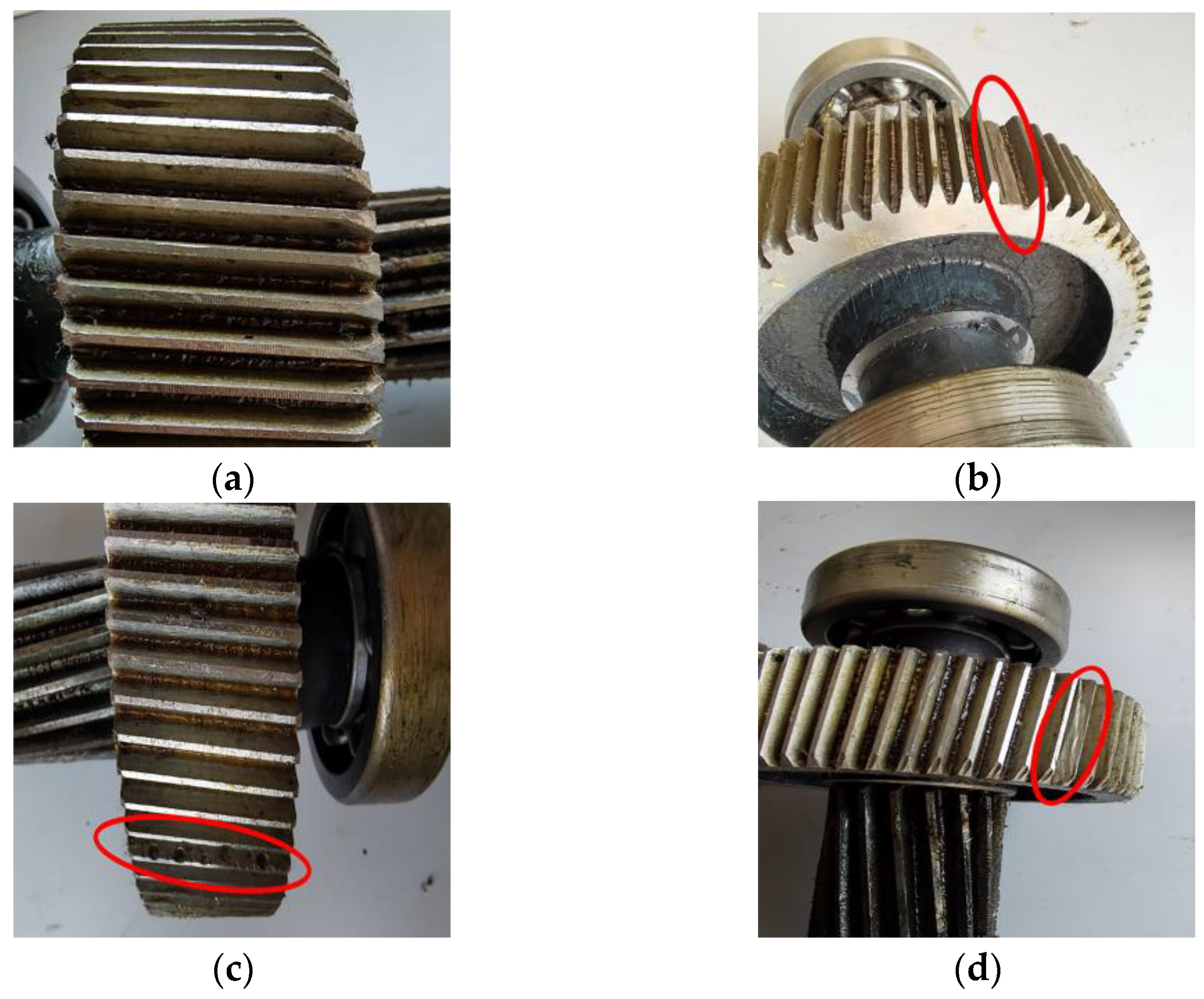
From Section 4.1 (Analysis of Typical Fault Forms of Gearboxes), it can be seen that the faults caused by gears account for the largest proportion, followed by bearing faults. There are not enough gear samples in this experiment, and gear failures caused by tooth fracture, pitting, and wear account for 82% of gear failures. Therefore, this paper mainly sets three failure forms of broken teeth: both the pitting and wear with the highest proportion of gear failures, and the one normal form that has a total of four states of gear samples for subsequent experimental development, data collection, and intelligent diagnosis. These are shown in Figure 4.

In Figure 4a–d, the four gear states of normal, broken, pitting, and wear, respectively, are shown. The breakage shown in Figure 4b is a serious form of gear failure, where generally one or more teeth of the gear is broken. When the gear is overloaded, eccentrically loaded, or subjected to a large impact during work, the teeth may break. Figure 4c shows an example that is prone to pitting failure on the root surface near the pitch line. The occurrence of gear pitting makes the meshing performance of the gears worse, which easily generates large vibrations. The wear in Figure 4d is mainly a failure form caused by insufficient lubrication or the entry of hard abrasives such as metal particles, dust, and metal oxides onto the working surface of the gear during transmission, resulting in severe wear on the gear contact surface.

4.2.3. Experimental Platform Construction

In order to complete the construction of the gear box fault experiment platform, the relevant experimental schemes were set up based on the abovementioned fault forms and the selected experimental equipment. The connection relationship of the relevant experimental equipment is shown in Figure 5.

It can be seen from Figure 5 that, during the experiment, the three-phase asynchronous motor, gearbox, and magnetic powder brake were first fixed on the test bench. The three-phase asynchronous motor was connected to the power supply through the frequency converter. The motor and the gearbox were connected by a pulley. The magnetic powder brake was connected with the gearbox through a coupling. The acceleration sensor was fixed on the bearing seats at both ends of the high-speed shaft of the gearbox and connected to the data acquisition card to transmit the acquired vibration data to the PC for analysis. Figure 6 shows the physical map of the gear box fault test platform.

In the experiment, the frequency converter was used to control and adjust the motor speed so as to realize the control and adjustment of the gearbox speed. The relationship between the motor speed and the output frequency of the inverter is shown in Formula (9):

$$v=\frac{1500f}{f_{\max }}$$

(9)

In Formula (9), $\nu$ is the motor speed and $f$ is the frequency adjusted by the inverter. The constant 1500 is the theoretical output maximum value of the motor selected in the experiment. $f_{\max }$ is the maximum value of the frequency converter output frequency, and $f_{\max }$ is taken as 50 Hz. The experimental information is shown in

Table 3. Experimental information.

Type	Gearbox Status	Motor Speed/Hz	Brake Load/A	Data Length	Number of Datasets
1	Broken	30	0.5	2048	300 × 2
2	Pitting	30	0.5	2048	300 × 2
3	Normal	30	0.5	2048	300 × 2
4	Wear	30	0.5	2048	300 × 2

.

It can be seen from Table 3 that the sampling frequency was set to 6 k Hz in this paper. The experimental load was set to 0.5 A through the magnetic powder brake controller. The data acquisition card and sensor were used to collect the vibration data when the speed was 900 r/min—that is, when the output power of the frequency converter was 30 Hz as the analysis object. A total of 300 groups were collected for each state, and since there are two sensor channels, the number of groups for each state is 300 × 2. The sample length of each group is 2048, and the four states total 1200 × 2 groups.

4.2.4. Experimental Data Design

The vibration signals of different positions of the gearbox obtained by Sensor 1 (Channel 1) and Sensor 2 (Channel 2) in the abovementioned gearbox fault diagnosis experiment platform were designed. The data introduction is shown in

Table 4. Data introduction.

Type	Gearbox Status	Number of Training Sets	Number of Validation Sets	Number of Test Sets	Label
1	Broken	180 × 2048 × 2	60 × 2048 × 2	60 × 2048 × 2	1 0 0 0
2	Pitting	180 × 2048 × 2	60 × 2048 × 2	60 × 2048 × 2	0 1 0 0
3	Normal	180 × 2048 × 2	60 × 2048 × 2	60 × 2048 × 2	0 0 1 0
4	Wear	180 × 2048 × 2	60 × 2048 × 2	60 × 2048 × 2	0 0 0 1

.

It can be seen from Table 4 that firstly, the vibration signals collected by the two acceleration sensors are constructed into a dual-channel sample. The training set, verification set, and test set were randomly divided according to a 6:2:2 ratio—that is, 180 sets of training, 60 sets of verification, and 60 sets of testing for each state of a single sensor. A total of 720 sets of training samples, 240 sets of verification samples, and 240 sets of test samples were obtained in the four states. There are 2048 points in each sample, thus the sample composition of each sensor channel is as follows: the training set structure is 720 × 2048; the validation set sample structure is 240 × 2048; and the test set sample structure is 240 × 2048. Two sensor samples of the same state of the gear are regarded as the same class. The labels of broken teeth, pitting, normal, and worn states as 1, 2, 3, and 4, respectively, were set. The labels were one-hot encoded—that is, the four labels 1, 2, 3, and 4 correspond to 1 0 0 0, 0 1 0 0, 0 0 1 0, and 0 0 0 1, respectively. Additionally, the dual-channel training samples were input into the model for training. The upper channel of PCNN receives samples from Sensor 1, and the lower channel receives samples from Sensor 2.

5. Experimental Analysis and Verification

5.1. Experimental Analysis

Through using the experimental data information in Table 3 and Table 4, the time-domain and frequency-domain diagrams of the vibration signals of the two channels and four states of the gearbox were obtained. These are shown in Figure 7 and Figure 8, respectively.

The time-domain plot of Figure 7 is a representation of a signal on a time axis, thus showing the amplitude of the signal as a function of time. The frequency-domain plot of Figure 8 is a representation of the signal on the frequency axis, showing the energy distribution of the signal at different frequencies. By decomposing a signal into its frequency components, it provides the frequency characteristics of the signal. From Figure 7 and Figure 8, it can be seen intuitively that the time-domain signals and frequency-domain signals received by Sensor 1 and Sensor 2, respectively, in the four states of the gearbox are evidently different and both present periodic fluctuations.

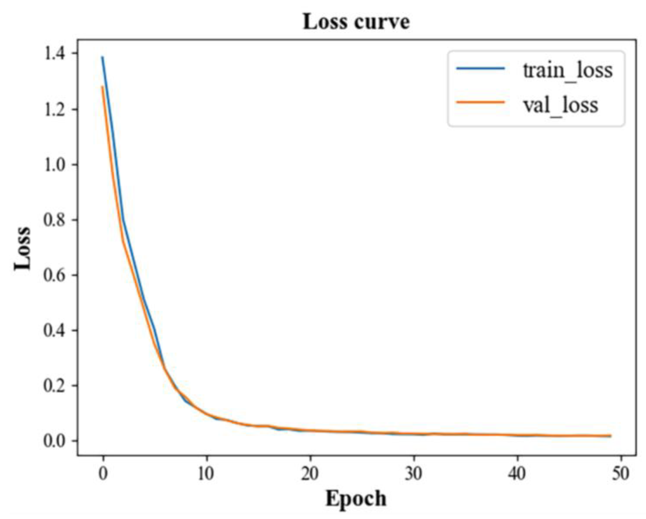
This experiment was run on a Windows 11 64-bit operating system with 8 GB of running memory. The software and hardware configuration conditions were as follows: Python version 3.10.4; the Spyder version 5.2.2; and TensorFlow version 2.9.1. The model training parameter settings were as follows: number of iterations was set to 50; batch_size set to 32; an Adam optimizer was used; the initial learning rate was set to 0.001; the learning rate decay value was set to 0.02; and the dropout ratio was set to 0.4. To avoid the effects of chance, the experiment process was repeated ten times. During the training process of one experiment, the accuracy change curves and loss rate change curves of the training and verification sets are shown in Figure 9 and Figure 10, respectively.

It can be seen from Figure 9 that, with the iterative process, the accuracy of the training set and the verification set were significantly improved. After the 20th iteration, it is essentially stable and tends to be flat. The accuracy curves of the training set and the verification set ultimately coincide after the 20th iteration, and the accuracy rates are both 1. It can be seen from the loss rate change curve in Figure 10 that the loss rate of the training set and the verification set gradually decreases with the increase in the number of iterations. Additionally, the values are essentially stabilized and leveled off after the 20th iteration. The loss rate curves of the training set and the verification set also essentially coincide after the 20th iteration, and the loss rate is close to 0. Through the analysis of the above two figures, the model is shown to converge well and that it has been fitted effectively.

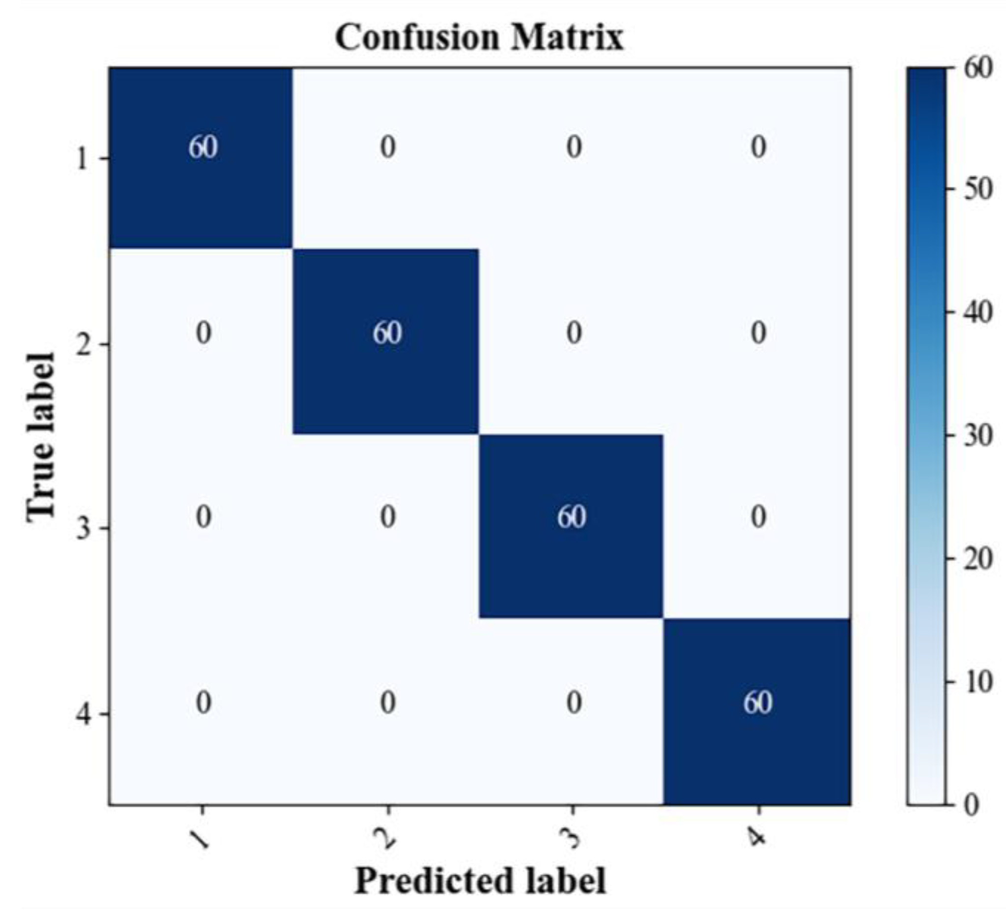
The test set was input into the trained model and the obtained test results were visualized through the confusion matrix. The confusion matrix of the test set is shown in Figure 11.

It can be seen from Figure 11 that all of the samples in the test set were recognized correctly and the overall recognition rate is 100%. It shows that the PCNN–GRU fault diagnosis model fused with multi-sensor information can effectively identify different fault states of the gearbox. In order to prevent the randomness of the results, the test results of the 10 experiments of the model are shown in

Table 5. Test results of ten experiments of PCNN–GRU

Number of Times	Loss Rate/%	Accuracy/%	Average Accuracy Rate/%	Average Loss Rate/%
1	0.06	100	99.92	0.09
2	0.11	99.58
3	0.11	100
4	0.18	100
5	0.04	99.58
6	0.13	100
7	0.18	100
8	0.03	100
9	0.09	100
10	0.01	100

.

It can be seen from Table 5 that the highest recognition rate in the 10 experiments is 100%, the lowest is 99.58%, and the average recognition rate is 99.92%. This shows that the PCNN–GRU fusion sensor information gearbox fault diagnosis method proposed in this paper has a good recognition effect.

5.2. t-SNE Visualization

t-SNE was used to visualize the output features of each layer during the testing process of the first experiment of the model. Figure 12 shows the feature distribution of different layers of the model.

It can be seen from Figure 12a,b that the distribution of the four states of raw data from different sensors greatly overlaps, and that different states cannot be effectively distinguished. It can be seen from Figure 12c,d that after the second layer of convolution, the raw data of Sensor 1 and Sensor 2 begin to gather in the same categories, but it is still difficult to distinguish them. It can be seen from Figure 12e,f that after fusing the features of the upper and lower channels of the convolutional neural network, the distinction of different categories of features and the aggregation of the same category of features are significantly improved. Additionally, after passing through the GRU layer, the four states can be clearly distinguished. As shown in Figure 12g, the final fusion features are effectively recognized at the recognition layer, and the four states are clearly distinguished. This is consistent with the final recognition results and the display of the confusion matrix. It shows that the PCNN–GRU method can mine useful features that can characterize the different fault states of gearboxes from vibration signals.

5.3. Comparison of Methods

In order to illustrate the effectiveness and advantages of the method in this paper, the PCNN–GRU method in this chapter is compared with the following methods:

(1)

PCNN: The vibration data of Sensor 1 and Sensor 2 were input into the PCNN;

(2)

Upper channel (Sensor 1) + CNN–GRU: Only the upper channel (Sensor 1) vibration signal was used to input into the CNN–GRU;

(3)

Lower channel (Sensor 2) + CNN–GRU: Only the lower channel (Sensor 2) vibration signal was used to input into the CNN–GRU;

(4)

Upper channel (Sensor 1) + CNN: Only the upper channel (Sensor 1) vibration signal was used to input into the CNN;

(5)

Lower channel (Sensor 2) + CNN: Only the vibration signal of the lower channel (Sensor 2) was used to input into the CNN.

Each method was independently trained and tested 10 times. The average recognition rate and average loss rate of the 10 diagnostic results by different methods are shown in

Table 6. The average recognition rate and average loss rate of 10 diagnostic results by different methods.

Method	Average Loss Rate of 10 Tests/%	Average Recognition Rate of 10 Tests/%
PCNN–GRU	0.09	99.92
PCNN	5.67	99.42
Sensor 1-CNN–GRU	9.32	96.84
Sensor 2-CNN–GRU	11.12	96.38
Sensor 1-CNN	17.84	94.96
Sensor 2-CNN	24.79	92.92

.

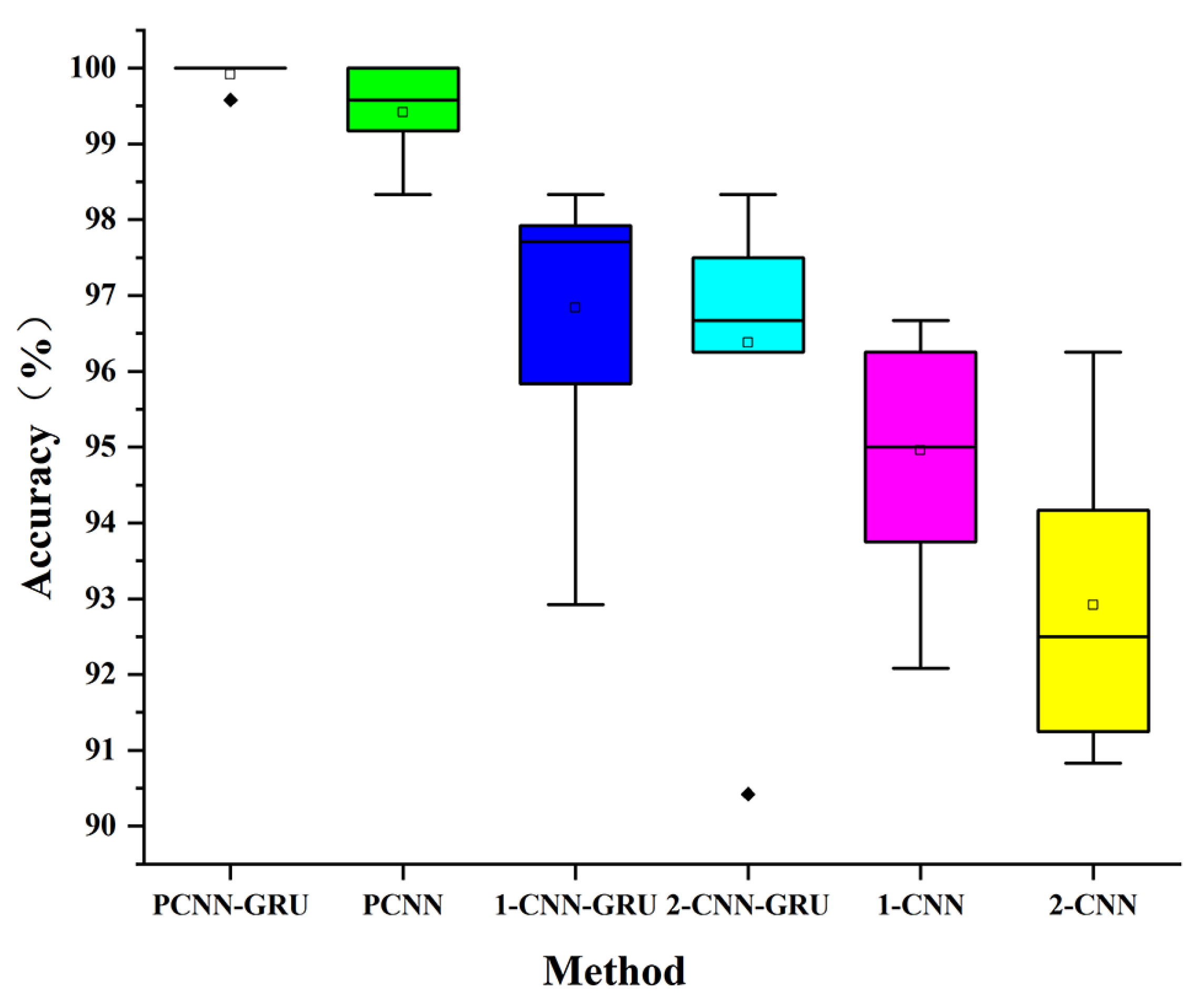
It can be seen from Table 6 that the PCNN–GRU fusion multi-sensor information gearbox fault diagnosis model proposed in this paper has the highest recognition rate of 99.92%. Additionally, the loss rate is also the lowest at 0.09% (the loss rate refers to the cross-entropy value between the prediction result and the actual value; the lower the loss rate, the closer the prediction result is to the real value, which indicates that the prediction effect of the model is better). Compared with the multi-sensor information fusion method when using only PCNN, the accuracy rate is increased by 0.5% and the loss rate is reduced by 5.58%. This shows that after using GRU to further extract the timing features of multiple sensors, not only has the accuracy rate been improved, but also the obtained results are closer to the actual value. Compared with the method based on a single sensor, the recognition rate has been effectively improved to varying degrees. It is also compared with some models mentioned in the introduction, such as WPD–CNN and LSTM model with cosine loss. Many tests have shown that the PCNN–GRU fusion multi-sensor information gearbox fault diagnosis model proposed in this paper has the highest recognition rate and the lowest loss rate. This shows that multi-sensor information fusion can more comprehensively characterize the fault characteristics of a gearbox, and it can effectively identify different fault states. The box plot of 10 diagnostic results by different methods is shown in Figure 13.

It can be seen from Figure 13 that the PCNN–GRU method in this chapter has a higher recognition rate than the other methods, and the results of the 10 tests are more concentrated. It also shows that the model recognition effect of the PCNN–GRU fusion multi-sensor information method is more stable, and that the fluctuation is smaller.

6. Conclusions

In this paper, a gearbox fault diagnosis method based on multi-sensor deep spatiotemporal feature representation is proposed. The vibration signals collected by the acceleration sensors at different positions in the gearbox fault test platform are input into the parallel CNN (PCNN) to mine the spatial information of the vibration signals. The fusion layer was used to fuse the spatial information of the different sensors. The GRU model was further used to extract the time series information in order to obtain the deep spatiotemporal features that fuse the spatial and temporal information of the multiple sensors. SoftMax was used for identification, and the intelligent diagnosis of the gearbox end-to-end was completed. The accuracy rate of the 10 tests was 99.92%, which is higher than those of the multi-sensor + parallel CNN and single-sensor-based diagnosis methods, and it also has a higher stability and lower loss rate. This proves that the PCNN–GRU fusion multi-sensor information fault diagnosis method is effective and superior.

References

1. Khan, A.; Hwang, H.; Kim, H.S. Synthetic Data Augmentation and Deep Learning for the Fault Diagnosis of Rotating Machines. Mathematics 2021, 9, 2336. [Google Scholar] [CrossRef]
2. Liang, X.; Zuo, M.J.; Feng, Z. Dynamic modeling of gearbox faults: A review. Mech. Syst. Signal Process. 2018, 98, 852–876. [Google Scholar] [CrossRef]
3. Khalid, S.; Hwang, H.; Kim, H.S. Real-World Data-Driven Machine-Learning-Based Optimal Sensor Selection Approach for Equipment Fault Detection in a Thermal Power Plant. Mathematics 2021, 9, 2814. [Google Scholar] [CrossRef]
4. Schmidt, S.; Heyns, P.S.; Gryllias, K.C. A methodology using the spectral coherence and healthy historical data to perform gearbox fault diagnosis under varying operating conditions. Appl. Acoust. 2020, 158, 107038. [Google Scholar] [CrossRef]
5. Jiang, Z.; Han, Q.; Xu, X. Fault diagnosis of planetary gearbox based on motor current signal analysis. Shock Vib. 2020, 2020, 8854776. [Google Scholar] [CrossRef]
6. Praveenkumar, T.; Saimurugan, M.; Krishnakumar, P.; Ramachandran, K.I. Fault diagnosis of automobile gearbox based on machine learning techniques. Procedia Eng. 2014, 97, 2092–2098. [Google Scholar] [CrossRef] [Green Version]
7. Saufi, S.R.; Ahmad, Z.A.B.; Leong, M.S.; Lim, M.H. Gearbox fault diagnosis using a deep learning model with limited data sample. IEEE Trans. Ind. Inform. 2020, 16, 6263–6271. [Google Scholar] [CrossRef]
8. Fan, X.; Zuo, M.J. Gearbox fault detection using Hilbert and wavelet packet transform. Mech. Syst. Signal Process. 2006, 20, 966–982. [Google Scholar] [CrossRef]
9. Feng, Z.; Zhu, W.; Zhang, D. Time-Frequency demodulation analysis via Vold-Kalman filter for wind turbine planetary gearbox fault diagnosis under nonstationary speeds. Mech. Syst. Signal Process. 2019, 128, 93–109. [Google Scholar] [CrossRef]
10. Yoon, J.; He, D.; Van Hecke, B. On the use of a single piezoelectric strain sensor for wind turbine planetary gearbox fault diagnosis. IEEE Trans. Ind. Electron. 2015, 62, 6585–6593. [Google Scholar] [CrossRef]
11. Singh, J.; Azamfar, M.; Ainapure, A.; Lee, J. Deep learning-based cross-domain adaptation for gearbox fault diagnosis under variable speed conditions. Meas. Sci. Technol. 2020, 31, 055601. [Google Scholar] [CrossRef]
12. Manikandan, S.; Duraivelu, K. Fault diagnosis of various rotating equipment using machine learning approaches–A review. Proc. Inst. Mech. Eng. Part E J. Process Mech. Eng. 2021, 235, 629–642. [Google Scholar] [CrossRef]
13. Xia, T.; Jiang, Y.; Zhuo, P.; Xi, L.; Wang, D. Dual-ensemble multi-feedback neural network for gearbox fault diagnosis. IEEE Trans. Instrum. Meas. 2021, 70, 3519610. [Google Scholar] [CrossRef]
14. Liao, Y.; Zhang, L.; Li, W. Regrouping particle swarm optimization based variable neural network for gearbox fault diagnosis. J. Intell. Fuzzy Syst. 2018, 34, 3671–3680. [Google Scholar] [CrossRef]
15. Zhang, X.; Han, P.; Xu, L.; Zhang, F.; Wang, Y.; Gao, L. Research on bearing fault diagnosis of wind turbine gearbox based on 1DCNN-PSO-SVM. IEEE Access 2020, 8, 192248–192258. [Google Scholar] [CrossRef]
16. Wang, Z.; Wang, J.; Wang, Y. An intelligent diagnosis scheme based on generative adversarial learning deep neural networks and its application to planetary gearbox fault pattern recognition. Neurocomputing 2018, 310, 213–222. [Google Scholar] [CrossRef]
17. Tong, S.; Li, J.; Cong, F.; Fu, Z.; Tong, Z. Vibration Separation Methodology Compensated by Time-Varying Transfer Function for Fault Diagnosis of Non-Hunting Tooth Planetary Gearbox. Sensors 2022, 22, 557. [Google Scholar] [CrossRef]
18. Jia, F.; Lei, Y.; Guo, L.; Lin, J.; Xing, S. A neural network constructed by deep learning technique and its application to intelligent fault diagnosis of machines. Neurocomputing 2018, 272, 619–628. [Google Scholar] [CrossRef]
19. Hinton, G.E.; Salakhutdinov, R.R. Reducing the dimensionality of data with neural networks. Science 2006, 313, 504–507. [Google Scholar] [CrossRef] [Green Version]
20. He, M.; He, D. Deep learning based approach for bearing fault diagnosis. IEEE Trans. Ind. Appl. 2017, 53, 3057–3065. [Google Scholar] [CrossRef]
21. Xu, Y.; Li, Z.; Wang, S.; Li, W.; Sarkodie-Gyan, T.; Feng, S. A hybrid deep-learning model for fault diagnosis of rolling bearings. Measurement 2021, 169, 108502. [Google Scholar] [CrossRef]
22. Huang, D.; Zhang, W.A.; Guo, F.; Liu, W.; Shi, X. Wavelet Packet Decomposition-Based Multiscale CNN for Fault Diagnosis of Wind Turbine Gearbox. IEEE Trans. Cybern. 2023, 53, 443–453. [Google Scholar] [CrossRef]
23. Jin, T.; Yan, C.; Chen, C.; Yang, Z.; Tian, H.; Wang, S. Light neural network with fewer parameters based on CNN for fault diagnosis of rotating machinery. Measurement 2021, 181, 109639. [Google Scholar] [CrossRef]
24. Yin, A.; Yan, Y.; Zhang, Z.; Li, C.; Sánchez, R.-V. Fault Diagnosis of Wind Turbine Gearbox Based on the Optimized LSTM Neural Network with Cosine Loss. Sensors 2020, 20, 2339. [Google Scholar] [CrossRef] [PubMed] [Green Version]
25. Miao, X.; Li, S.; Zhu, Y.; An, Z. A novel real-time fault diagnosis method for planetary gearbox using transferable hidden layer. IEEE Sens. J. 2020, 20, 8403–8412. [Google Scholar] [CrossRef]
26. Du, Z.; Fan, B.; Chi, J.; Jin, X. Sensor fault detection and its efficiency analysis in air handling unit using the combined neural networks. Energy Build. 2014, 72, 157–166. [Google Scholar] [CrossRef]
27. Hussain, S.; Mokhtar, M.; Howe, J.M. Sensor failure detection, identification, and accommodation using fully connected cascade neural network. IEEE Trans. Ind. Electron. 2014, 62, 1683–1692. [Google Scholar] [CrossRef]
28. Wang, H.; Xu, J.; Yan, R.; Sun, C.; Chen, X. Intelligent bearing fault diagnosis using multi-head attention-based CNN. Procedia Manuf. 2020, 49, 112–118. [Google Scholar] [CrossRef]
29. Chen, J.; Jiang, J.; Guo, X.; Tan, L. A self-Adaptive CNN with PSO for bearing fault diagnosis. Syst. Sci. Control Eng. 2021, 9, 11–22. [Google Scholar] [CrossRef]
30. Li, H.; Zhang, Q.; Qin, X.; Sun, Y. K-SVD-based WVD enhancement algorithm for planetary gearbox fault diagnosis under a CNN framework. Meas. Sci. Technol. 2019, 31, 025003. [Google Scholar] [CrossRef]
31. Jiang, J.; Bie, Y.; Li, J.; Yang, X.; Ma, G.; Lu, Y.; Zhang, C. Fault diagnosis of the bushing infrared images based on mask R-CNN and improved PCNN joint algorithm. High Volt. 2021, 6, 116–124. [Google Scholar] [CrossRef]
32. Ruan, D.; Song, X.; Gühmann, C.; Yan, J. Collaborative optimization of CNN and GAN for bearing fault diagnosis under unbalanced datasets. Lubricants 2021, 9, 105. [Google Scholar] [CrossRef]
33. Liu, Y.; Chen, C.; Wang, T.; Cheng, L. An attention enhanced dilated CNN approach for cross-axis industrial robotics fault diagnosis. Auton. Intell. Syst. 2022, 2, 11. [Google Scholar] [CrossRef]
34. Wang, J.; Yang, J.; Wang, Y.; Bai, Y.; Zhang, T.; Yao, D. Ensemble decision approach with dislocated time–frequency representation and pre-trained CNN for fault diagnosis of railway vehicle gearboxes under variable conditions. Int. J. Rail Transp. 2022, 10, 655–673. [Google Scholar] [CrossRef]
35. Ma, Y.; Jia, X.; Bai, H.; Liu, G.; Wang, G.; Guo, C.; Wang, S. A new fault diagnosis method based on convolutional neural network and compressive sensing. J. Mech. Sci. Technol. 2019, 33, 5177–5188. [Google Scholar] [CrossRef]
36. Liu, H.; Ma, R.; Li, D.; Yan, L.; Ma, Z. Machinery fault diagnosis based on deep learning for time series analysis and knowledge graphs. J. Signal Process. Syst. 2021, 93, 1433–1455. [Google Scholar] [CrossRef]
37. Tao, Y.; Wang, X.; Sánchez, R.V.; Yang, S.; Bai, Y. Spur gear fault diagnosis using a multilayer gated recurrent unit approach with vibration signal. IEEE Access 2019, 7, 56880–56889. [Google Scholar] [CrossRef]
38. Guo, S.; Zhang, B.; Yang, T.; Lyu, D.; Gao, W. Multitask convolutional neural network with information fusion for bearing fault diagnosis and localization. IEEE Trans. Ind. Electron. 2019, 67, 8005–8015. [Google Scholar] [CrossRef]
39. Xu, Z.; Bashir, M.; Zhang, W.; Yang, Y.; Wang, X.; Li, C. An intelligent fault diagnosis for machine maintenance using weighted soft-voting rule based multi-attention module with multi-scale information fusion. Inf. Fusion 2022, 86, 17–29. [Google Scholar] [CrossRef]
40. Aherwar, A. An investigation on gearbox fault detection using vibration analysis techniques: A review. Aust. J. Mech. Eng. 2012, 10, 169–183. [Google Scholar] [CrossRef]
41. Chen, J.P.; Wang, Y.L.; Zhao, C.X.; Li, X. Failure Analysis and Preventive Measures of Cooling Tower Fan Gearbox. Adv. Mater. Res. 2014, 989, 3302–3305. [Google Scholar] [CrossRef]
42. Fischer, K.; Besnard, F.; Bertling, L. Reliability-centered maintenance for wind turbines based on statistical analysis and practical experience. IEEE Trans. Energy Convers. 2011, 27, 184–195. [Google Scholar] [CrossRef] [Green Version]
Figure 1. GRU structure diagram.
Mathematics 11 02679 g001
Figure 2. The PCNN–GRU model structure diagram.
Mathematics 11 02679 g002
Figure 3. Overall flowchart of the fault diagnosis model.
Mathematics 11 02679 g003
Figure 4. Gear fault setting: (a) normal; (b) broken; (c) pitting; and (d) wear.
Mathematics 11 02679 g004
Figure 5. Experimental equipment connection diagram.
Mathematics 11 02679 g005
Figure 6. The physical picture of the gear box fault experiment platform.
Mathematics 11 02679 g006
Figure 7. Gearbox data time-domain diagram.
Mathematics 11 02679 g007
Figure 8. Gearbox data frequency-domain plot.
Mathematics 11 02679 g008
Figure 9. Accuracy change curve.
Mathematics 11 02679 g009
Figure 10. Loss rate change curve.
Mathematics 11 02679 g010
Figure 11. Confusion matrix of the test results.
Mathematics 11 02679 g011
Figure 12. Distribution of the features in each layer of the PCNN−GRU model: (a) feature distribution of the upper channel raw data; (b) the lower channel raw data feature distribution; (c) the convolution layer 2–1 feature distribution; (d) the convolution layer 2−2 feature distribution; (e) the feature distribution of the fusion layer; (f) the feature distribution of GRU layers; and (g) the output layer feature distribution.
Mathematics 11 02679 g012
Figure 13. Box plot for the results of the 10 tests.
Mathematics 11 02679 g013