
Exploration of New Solitons for the Fractional Perturbed Radhakrishnan–Kundu–Lakshmanan Model


Abstract
:1. Introduction
2. The Conformable Derivative
- (1)
- , for all
- (2)
- for all
- (3)
- (4)
- (5)
- If is differentiable, then
- (6)
- , for all constant functions
- (7)
- Chain rule: Let be a differentiable and —differerentiable function then the chain rule is given by:
3. Initial Information
Applying Wave Transformation to the Given Model
4. Description of the Adopted Methods
4.1. Mse Technique
4.2. Erf Technique
5. Application of the Given Methods
5.1. Mse Technique
5.2. Erf Technique
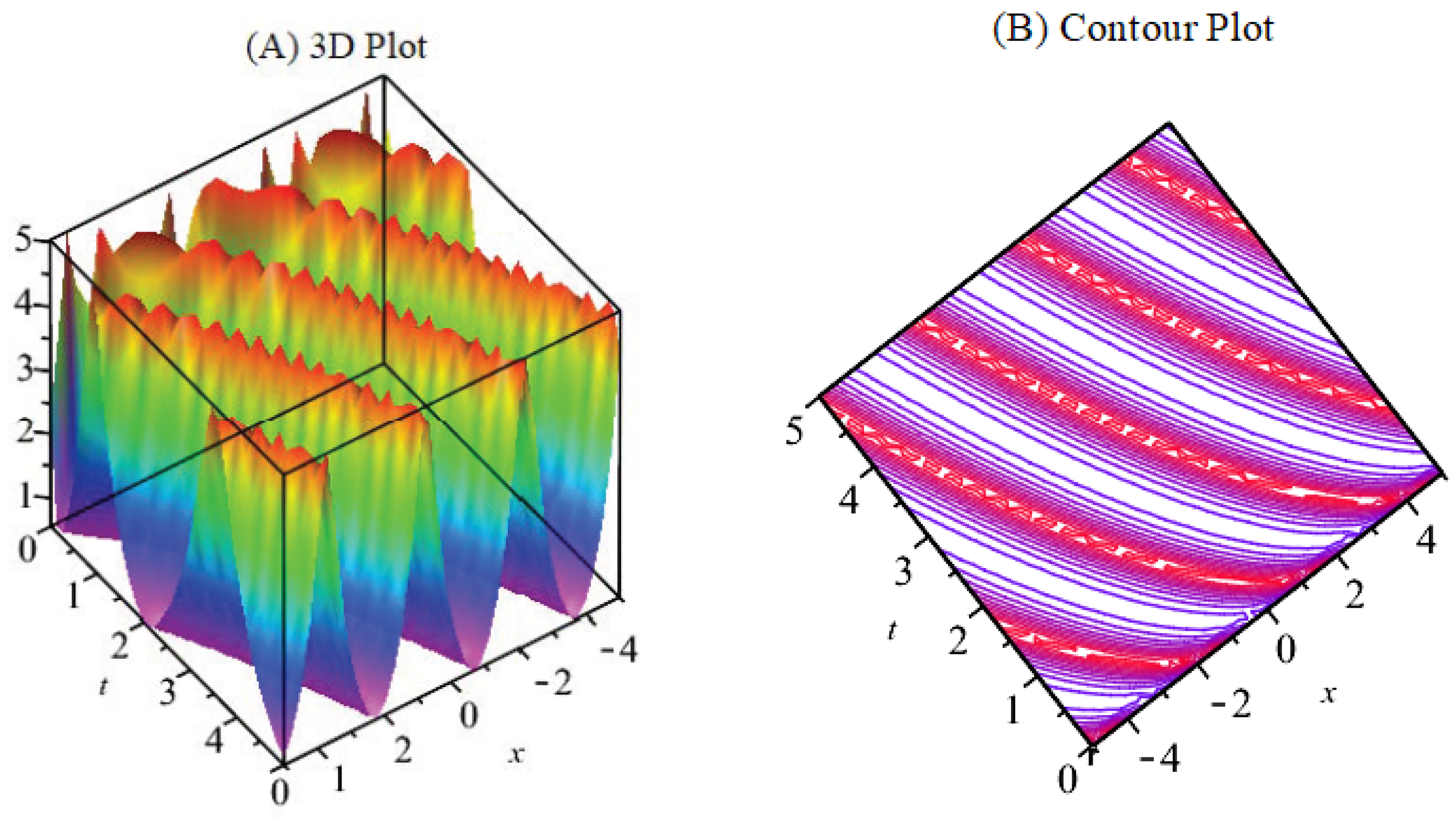
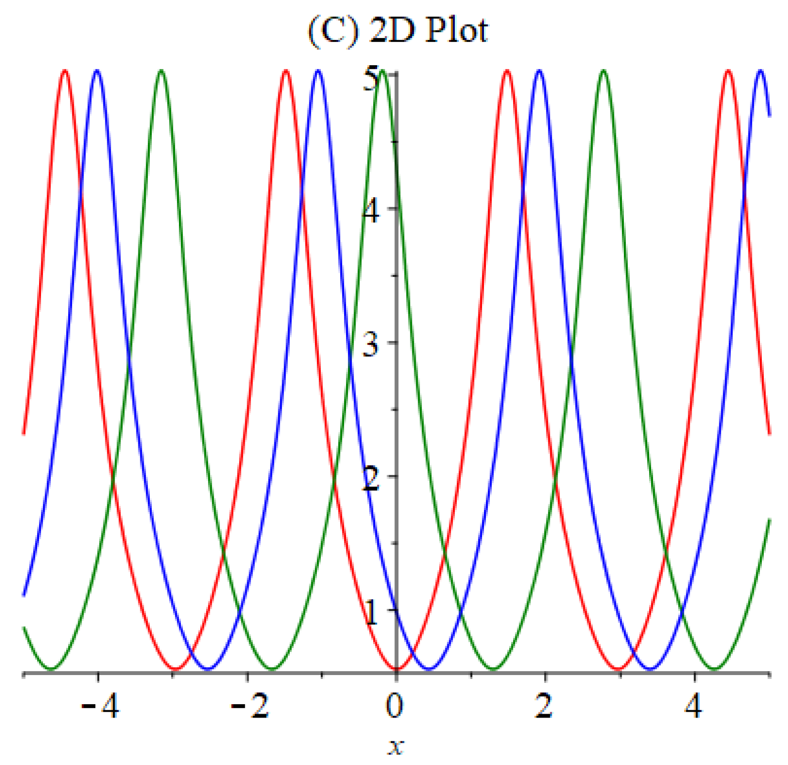
6. Discussion
7. Conclusions
Author Contributions
Funding
Data Availability Statement
Acknowledgments
Conflicts of Interest
References
- Sahadevan, R.; Bakkyaraj, T. Invariant Subspace Method and Exact Solutions of Certain Nonlinear Time Fractional Partial Differential Equations. Fract. Calc. Appl. Anal. 2015, 18, 146–162. [Google Scholar] [CrossRef]
- Prakash, P. Invariant subspaces and exact solutions for some types of scalar and coupled time-space fractional diffusion equations. Pramana 2020, 94, 103. [Google Scholar] [CrossRef]
- Cheng, X.; Hou, J.; Wang, L. Lie symmetry analysis, invariant subspace method and q-homotopy analysis method for solving fractional system of single-walled carbon nanotube. Comput. Appl. Math. 2021, 40, 103. [Google Scholar] [CrossRef]
- Agarwal, R.P.; Alghamdi, A.M.; Gala, S.; Ragusa, M.A. On the regularity criterion on one velocity component for the micropolar fluid equations. Math. Model. Anal. 2023, 28, 271–284. [Google Scholar] [CrossRef]
- El-Hady, E.; Makhlouf, A.B.; Boulaaras, S.; Mchiri, L. Ulam-Hyers-Rassias stability of non-linear differential equations with Riemann-Liouville fractional derivative. J. Funct. Spaces 2022, 2022, 7827579. [Google Scholar]
- Alatwi, R.S.E.; Aljohani, A.P.; Ebaid, A.; Al-Jeaid, H.K. Two analytical techniques for fractional differential equations with harmonic terms via the Riemann-Liouville definition. Mathematics 2022, 10, 4564. [Google Scholar] [CrossRef]
- Kumar, D.; Hosseini, K.; Kaabar, M.K.A.; Kaplan, M.; Salahshour, S. On some novel solution solutions to the generalized Schrödinger-Boussinesq equations for the interaction between complex short wave and real long wave envelope. J. Ocean. Eng. Sci. 2022, 7, 353–362. [Google Scholar] [CrossRef]
- Akinyemi, L.; Mirzazadeh, M.; Hosseini, K. Solitons and other solutions of perturbed nonlinear Biswas-Milovic equation with Kudryashov’s law of refractive index. Nonlinear Anal. Model. Control 2022, 27, 479–495. [Google Scholar] [CrossRef]
- Hosseini, K.; Akbulut, A.; Baleanu, D.; Salahshour, S.; Mirzazadeh, M.; Dehingia, K. The Korteweg-de Vries-Caudrey-Dodd-Gibbon dynamical model: Its conservation laws, solitons, and complexiton. J. Ocean Eng. Sci. 2022. [Google Scholar] [CrossRef]
- Akbulut, A.; Kaplan, M.; Kumar, D.; Tascan, F. The analysis of conservation laws, symmetries and solitary wave solutions of Burgers-Fisher equation. Int. J. Mod. Phys. B 2021, 35, 2150224. [Google Scholar] [CrossRef]
- Raza, N.; Rafiq, M.H.; Bekir, A.; Rezazadeh, H. Optical solitons related to (2+1)-dimensional Kundu-Mukherjee-Naskar model using an innovative integration architecture. J. Nonlinear Opt. Phys. Mater. 2022, 31, 2250014. [Google Scholar] [CrossRef]
- Sadaf, M.; Arshed, S.; Akram, G.; Iqra. A variety of solitary waves solutions for the modified nonlinear Schrödinger equation with conformable fractional derivative. Opt. Quantum Electron. 2023, 55, 372. [Google Scholar] [CrossRef]
- Alharthi, M.S.; Ali, H.M.S.; Habib, M.A.; Miah, M.M.; Aljohani, A.F.; Akbar, M.A.; Mahmoud, W.; Osman, M.S. Assorted soliton wave solutions of time-fractional BBM-Burger and Sharma-Tasso-Olver equations in nonlinear analysis. J. Ocean. Eng. Sci. 2023; in press. [Google Scholar] [CrossRef]
- Osman, M.S.; Baleanu, D.; Tariq, K.U.; Kaplan, M.; Younis, M.; Rizvi, S.T. Different types of progressive wave solutions via the 2D-chiral nonlinear Schrödinger equation. Front. Phys. 2020, 8, 215. [Google Scholar] [CrossRef]
- Biswas, A.; Yildirim, Y.; Yasar, E.; Mahmood, M.F.; Alshomrani, A.S.; Zhou, Q.; Moshokoa, S.P.; Belic, M. Optical soliton perturbation for Radhakrishnan-Kundu-Lakshmanan equation with a couple integration schemes. Optik 2018, 163, 126–136. [Google Scholar] [CrossRef]
- Chun-Gang, X.; Jian-Cheng, J.; Jia-Hua, H. New soliton solution of the generalized RKL equation through optical fiber transmission. J. Anhui Univ. 2011, 35, 39–47. [Google Scholar]
- Biswas, A. 1-soliton solution of the generalized Radhakrishnan, Kundu, Lakshmanan equation. Phys. Lett. A 2009, 373, 2546–2548. [Google Scholar] [CrossRef]
- Sturdevant, B.; Lott, D.A.; Biswas, A. Topological 1-soliton solution of the generalized Radhakrishnan-Kundu-Lakshmanan equation with nonlinear dispersion. Mod. Phys. Lett. B 2010, 24, 1825–1831. [Google Scholar] [CrossRef]
- Samko, G.; Kilbas, A.A.; Marichev, O.I. Fractional Integrals and Derivatives: Theory and Applications; Gordon and Breach: Yverdon, Switzerland, 1993. [Google Scholar]
- Kilbas, A.; Srivastava, M.H.; Trujillo, J.J. Theory and Application of Fractional Differential Equations. In North Holland Mathematics Studies; Elsevier: Amsterdam, The Netherlands, 2006; Volume 204. [Google Scholar]
- Khalil, R.; Horani, M.A.; Yousef, A.; Sababheh, M. A new definition of fractional derivative. J. Comput. Appl. Math. 2014, 264, 65–70. [Google Scholar] [CrossRef]
- Abdeljawad, T. On conformable fractional calculus. J. Comput. Appl. Math. 2015, 279, 57–66. [Google Scholar] [CrossRef]
- Benkhettou, N.; Hassani, S.; Torres, D.F.M. A conformable fractional calculus on arbitrary time scales. J. King Saud Univ. Sci. 2016, 28, 93–98. [Google Scholar] [CrossRef]
- Chung, W.S. Fractional Newton mechanics with conformable fractional derivative. J. Comput. Appl. Math. 2015, 290, 150–158. [Google Scholar] [CrossRef]
- Ghany, H.A.; Babb, A.S.O.E.; Zabel, A.M.; Hyder, A. The fractional coupled KdV equations: Exact solutions and white noise functional approach. Chin. Phys. B 2013, 22, 080501. [Google Scholar] [CrossRef]
- Ghany, H.A.; Hyder, A. Abundant solutions of Wick-type stochastic fractional 2D KdV equations. Chin. Phys. B 2014, 23, 060503. [Google Scholar] [CrossRef]
- Baleanu, D.; Guvenc, Z.B.; Machado, J.A.T. New Trends in Nanotechnology and Fractional Calculus Applications; Springer: Berlin/Heidelberg, Germany, 2010. [Google Scholar]
- Ullah, M.S.; Roshid, H.O.; Alshammari, F.S.; Ali, M.Z. Collision phenomena among the solitons, periodic and Jacobi elliptic functions to a (3+1)-dimensional Sharma-Tasso-Olver-like model. Results Phys. 2022, 36, 105412. [Google Scholar] [CrossRef]
- Khan, K.; Akbar, M.A.; Ali, N.H.M. The Modified Simple Equation Method for Exact and Solitary Wave Solutions of Nonlinear Evolution Equation: The GZK-BBM Equation and Right-Handed Noncommutative Burgers Equations. ISRN Math. Phys. 2013, 2013, 146704. [Google Scholar] [CrossRef]
- Akbulut, A.; Kaplan, M.; Kaabar, M.K.A. New conservation laws and exact solutions of the special case of the fifth-order KdV equation. J. Ocean. Eng. Sci. 2022, 7, 377–382. [Google Scholar] [CrossRef]
- Fadhal, E.; Akbulut, A.; Kaplan, M.; Awadalla, M.; Abuasbeh, K. Extraction of Exact So-lutions of Higher Order Sasa-Satsuma Equation in the Sense of Beta Derivative. Symmetry 2022, 14, 2390. [Google Scholar] [CrossRef]
- Mohyud-Din, S.T.; Bibi, S. Exact solutions for nonlinear fractional differential equations using exponential rational function method. Opt. Quantum Electron. 2017, 49, 64. [Google Scholar] [CrossRef]
- Ghanbari, B.; Gómez-Aguilar, J.F. The generalized exponential rational function method for Radhakrishnan-Kundu-Lakshmanan equation with beta-conformable time derivative. Rev. Mex. Física 2019, 65, 5. [Google Scholar]
- Ozdemir, N.; Esen, H.; Secer, A.; Bayram, M.; Sulaiman, T.A.; Yusuf, A.; Aydin, H. Optical solitons and other solutions to the Radhakrishnan-Kundu-Lakshmanan equation. Optik 2021, 242, 167363. [Google Scholar] [CrossRef]
- Sulaiman, T.A.; Bulut, H.; Yel, G.; Atas, S.S. Optical solitons to the fractional perturbed Radhakrishnan-Kundu-Lakshmanan model. Opt. Quantum Electron. 2018, 50, 372. [Google Scholar] [CrossRef]

Disclaimer/Publisher’s Note: The statements, opinions and data contained in all publications are solely those of the individual author(s) and contributor(s) and not of MDPI and/or the editor(s). MDPI and/or the editor(s) disclaim responsibility for any injury to people or property resulting from any ideas, methods, instructions or products referred to in the content. |
© 2023 by the authors. Licensee MDPI, Basel, Switzerland. This article is an open access article distributed under the terms and conditions of the Creative Commons Attribution (CC BY) license (https://creativecommons.org/licenses/by/4.0/).
Share and Cite
Kaplan, M.; Alqahtani, R.T. Exploration of New Solitons for the Fractional Perturbed Radhakrishnan–Kundu–Lakshmanan Model. Mathematics 2023, 11, 2562. https://doi.org/10.3390/math11112562
Kaplan M, Alqahtani RT. Exploration of New Solitons for the Fractional Perturbed Radhakrishnan–Kundu–Lakshmanan Model. Mathematics. 2023; 11(11):2562. https://doi.org/10.3390/math11112562
Chicago/Turabian StyleKaplan, Melike, and Rubayyi T. Alqahtani. 2023. "Exploration of New Solitons for the Fractional Perturbed Radhakrishnan–Kundu–Lakshmanan Model" Mathematics 11, no. 11: 2562. https://doi.org/10.3390/math11112562
APA StyleKaplan, M., & Alqahtani, R. T. (2023). Exploration of New Solitons for the Fractional Perturbed Radhakrishnan–Kundu–Lakshmanan Model. Mathematics, 11(11), 2562. https://doi.org/10.3390/math11112562