
Feature Selection Using Golden Jackal Optimization for Software Fault Prediction

 , ,
, ,  , and
, and
Abstract
:1. Introduction
2. Literature Review
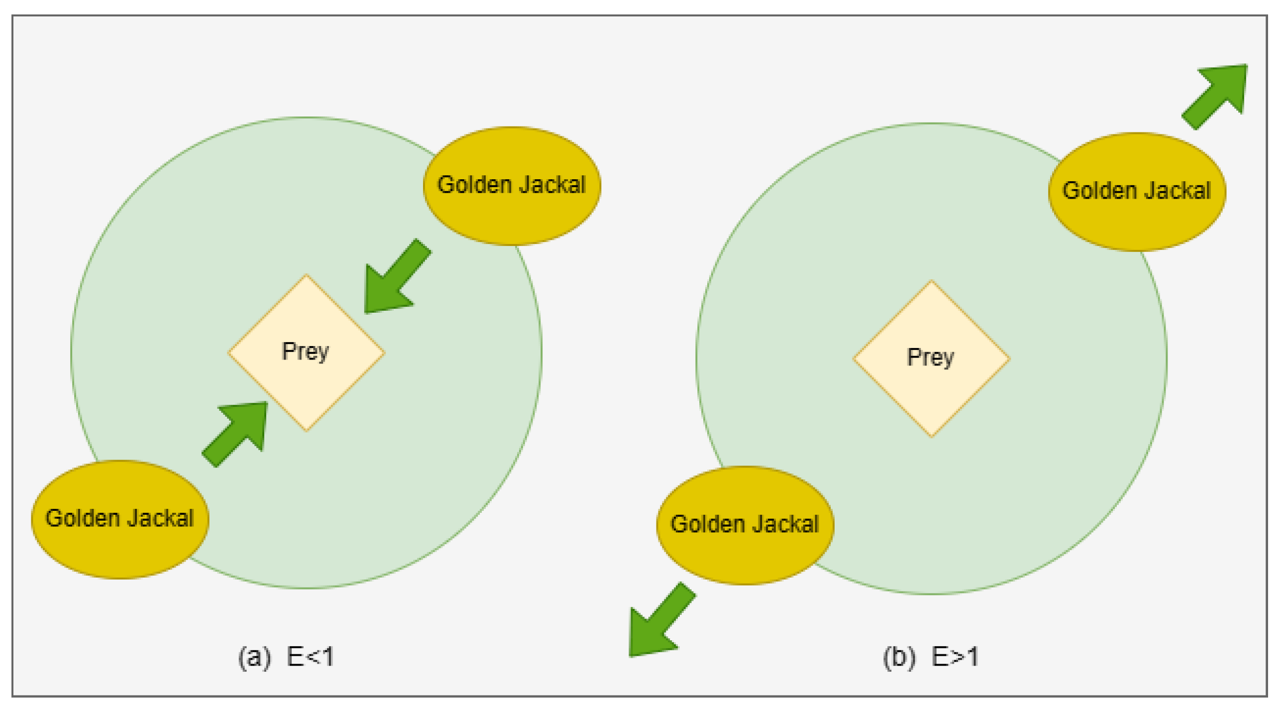
3. Summary of Golden Jackal Optimization Algorithm
- Locating the prey and advancing towards it.
- Trapping the prey and agitating it.
- Attacking and capturing the prey.
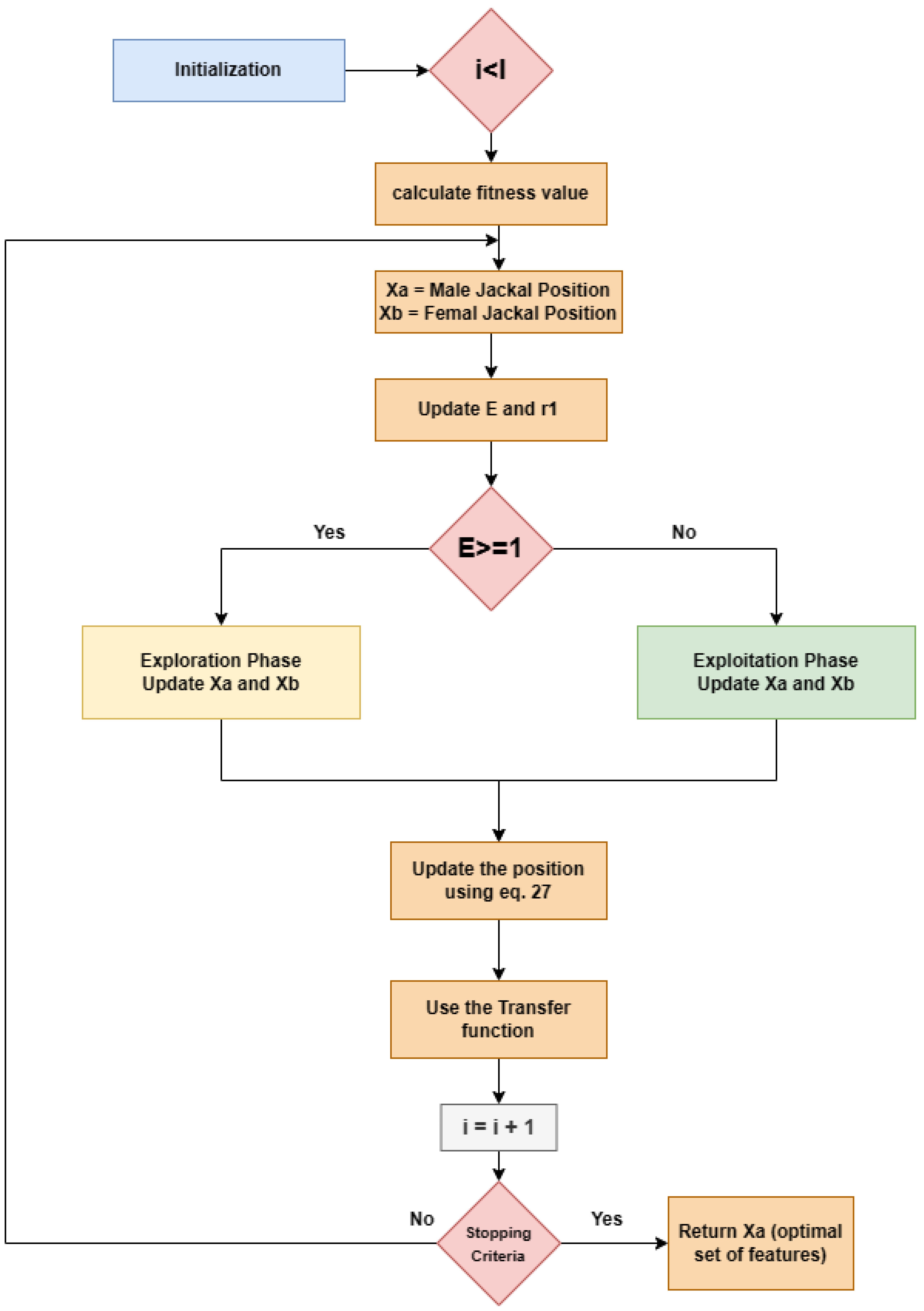
4. Feature Selection Using Golden Jackal Optimization
4.1. Initialization
4.2. Exploration Phase
4.3. Exploitation Phase
4.4. Fitness and Transfer Function
| Algorithms 1 FSGJO |
| 1. Initialize prey population randomly, 2. while () 3. Let, Male Jackal Position be 4. Let, Female Jackal Position be 5. Determine the preys’ fitness value 6. if () 7. 8. if ( and ) 9. 10. for (each prey) 11. Using Equations (21)–(23) update the evading energy ) 12. Using Equations (24) and (25) Update 13. if (E ≥ 1) (Exploration phase) 14. Using Equations (19), (20) and (27) Update the prey position 15. if (E < 1) (Exploration phase) 16. Using Equations (27)–(29) Update the prey position 17. Update Jackal Position, 18. Using transfer function to convert continuous values of i.e., position, in binary values using Equation (30) 19. end for 20. i++ 21. end while 22. Return Male Jackal Position |
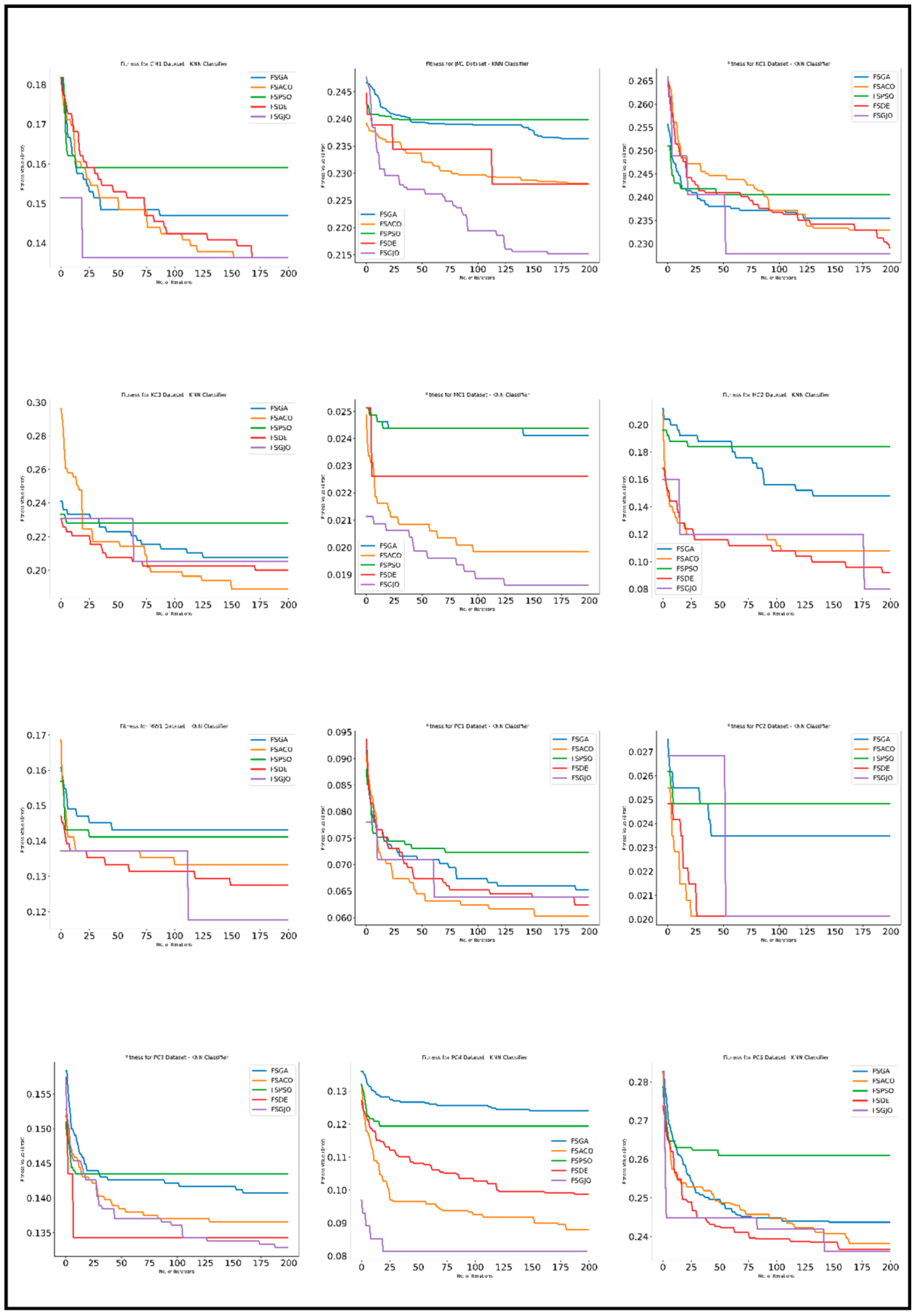
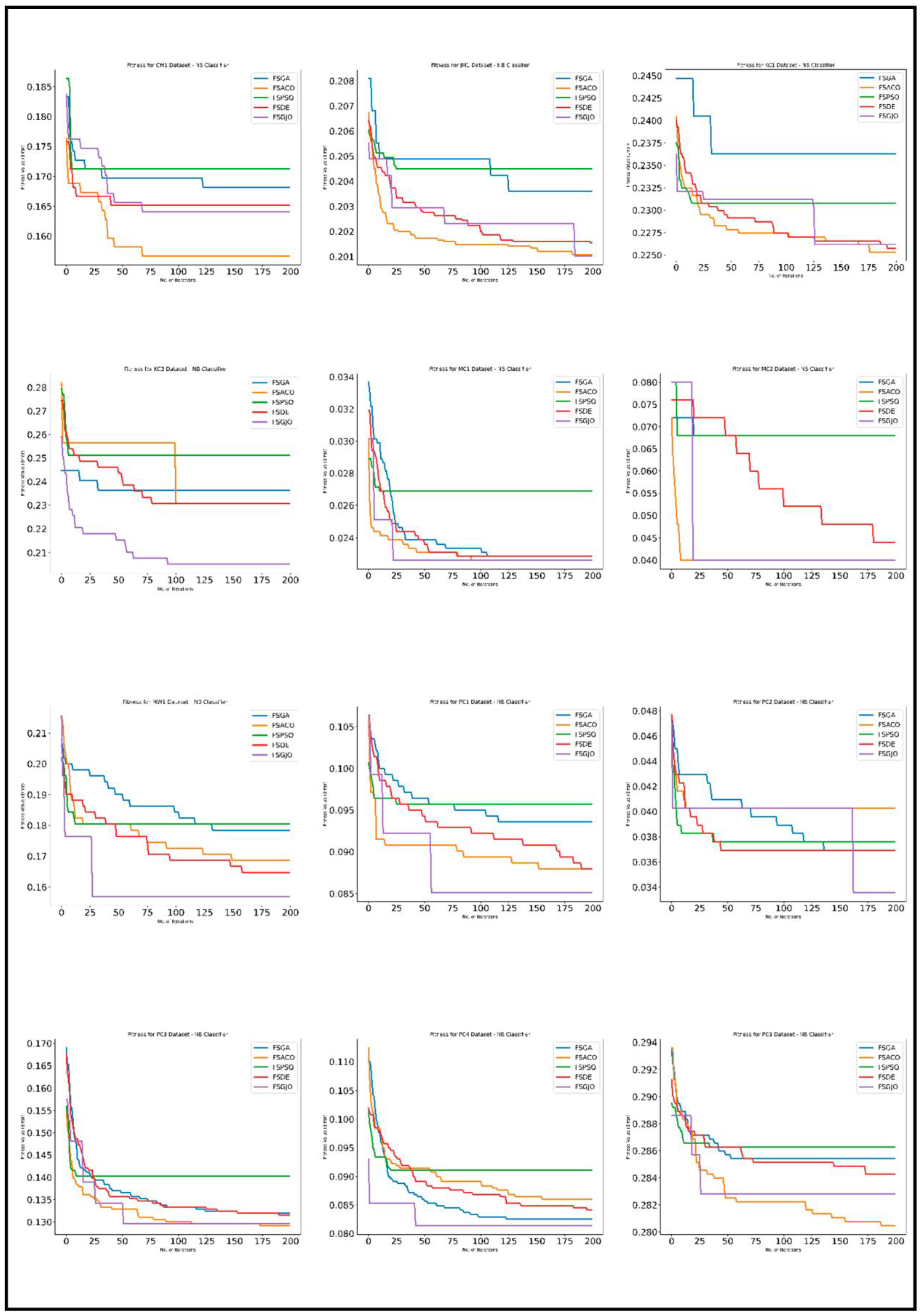
5. Results
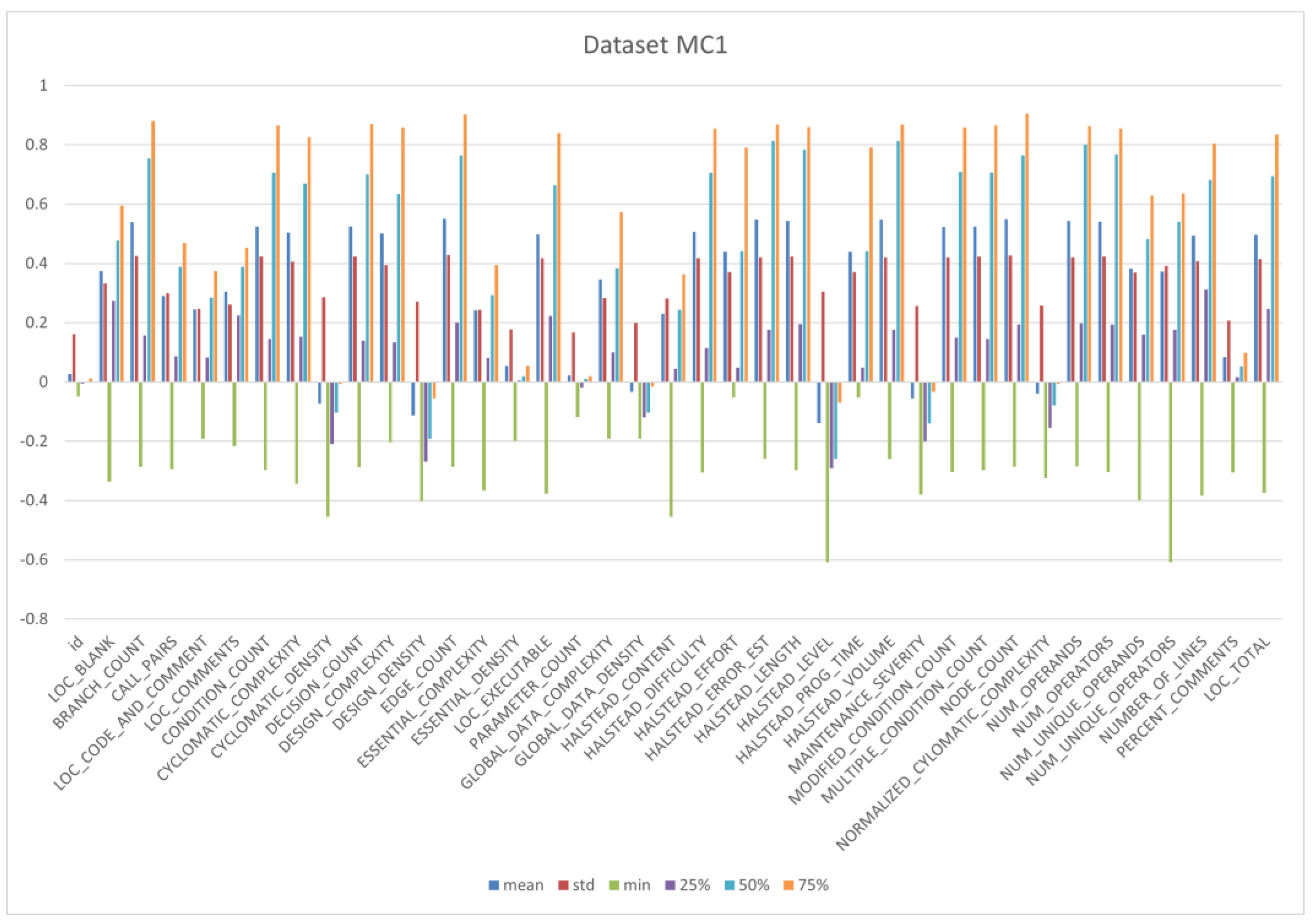
5.1. Datasets
- LOC (Lines of Code): This metric measures the number of lines of code in the software being analyzed.
- Cyclomatic Complexity: This metric measures the complexity of the software’s control flow and can help identify potential trouble spots.
- Code Churn: This metric measures the software’s change over time and can help identify modules or components that may be more prone to faults.
- Code Coverage: This metric measures the extent to which the software’s code has been tested and can help identify code areas that may be more likely to contain faults.
- Halstead’s Complexity Measures: These metrics measure various aspects of the complexity of the software’s code, such as the number of distinct operators and operands, and can help identify potential trouble spots.
5.2. Experimental Condition
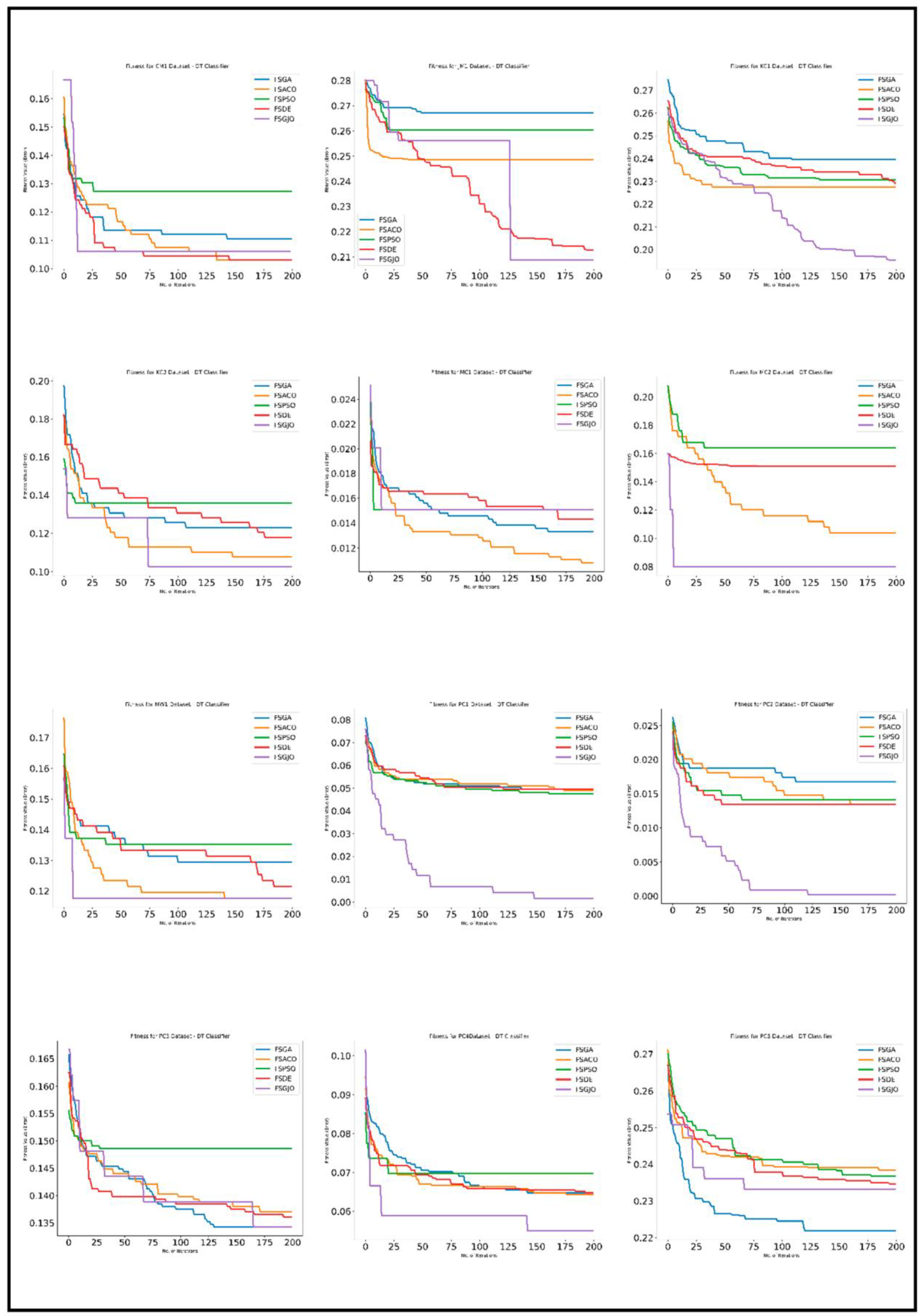
5.3. Experimental Analysis
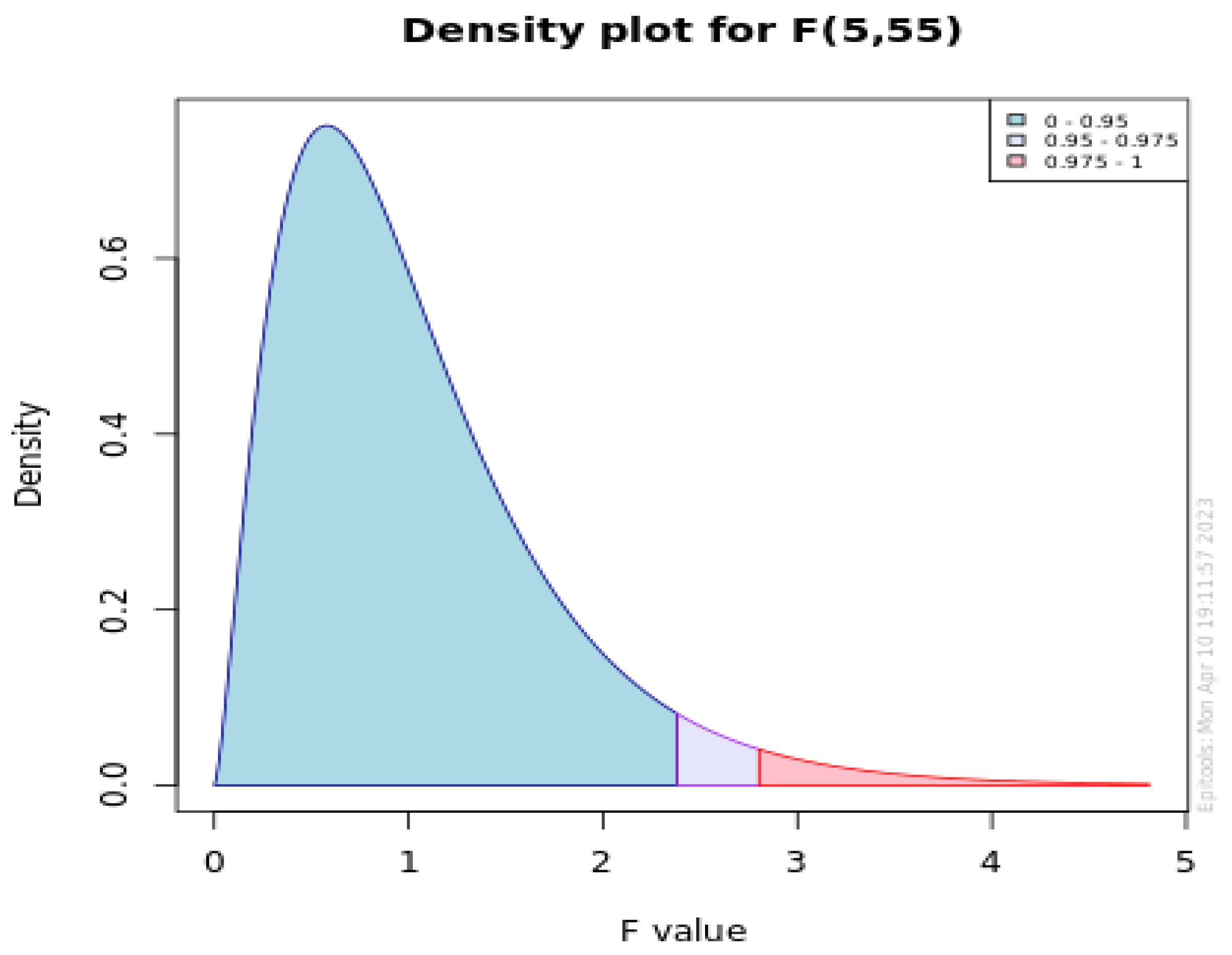
6. Statistical Analysis
7. Conclusions
Author Contributions
Funding
Data Availability Statement
Conflicts of Interest
References
- Catal, C. Software fault prediction: A literature review and current trends. Expert Syst. Appl. 2011, 38, 4626–4636. [Google Scholar] [CrossRef]
- Kundu, A.; Dutta, P.; Ranjit, K.; Bidyadhar, S.; Gourisaria, M.K.; Das, H. Software Fault Prediction Using Machine Learning Models. In Proceedings of the 2022 OITS International Conference on Information Technology (OCIT), Bhubaneswar, India, 14–16 December 2022; IEEE: Manhattan, NY, USA, 2022; pp. 170–175. [Google Scholar]
- Malhotra, R. Comparative analysis of statistical and machine learning methods for predicting faulty modules. Appl. Soft Comput. 2014, 21, 286–297. [Google Scholar] [CrossRef]
- Gm, H.; Gourisaria, M.K.; Pandey, M.; Rautaray, S.S. A comprehensive survey and analysis of generative models in machine learning. Comput. Sci. Rev. 2020, 38, 100285. [Google Scholar] [CrossRef]
- Rathore, S.S.; Kumar, S. A decision tree logic based recommendation system to select software fault prediction techniques. Computing 2017, 99, 255–285. [Google Scholar] [CrossRef]
- Rathore, S.S.; Kumar, S. A Decision Tree Regression based Approach for the Number of Software Faults Prediction. ACM SIGSOFT Softw. Eng. Notes 2016, 41, 1–6. [Google Scholar] [CrossRef]
- Singh, Y.; Kaur, A.; Malhotra, R. Software fault proneness prediction using support vector machines. In Proceedings of the World Congress on Engineering, London, UK, 1–3 July 2009; Volume 1, pp. 1–3. [Google Scholar]
- Li, J.; He, P.; Zhu, J.; Lyu, M.R. Software defect prediction via convolutional neural network. In Proceedings of the 2017 IEEE International Conference on Software Quality, Reliability and Security (QRS), Prague, Czech Republic, 25–29 July 2017; IEEE: Manhattan, NY, USA, 2017; pp. 318–328. [Google Scholar]
- Goyal, J.; Ranjan Sinha, R. Software defect-based prediction using logistic regression: Review and challenges. In Proceedings of the Second International Conference on Sustainable Technologies for Computational Intelligence: Proceedings of ICTSCI 2021, Dehradun, India, 22–23 May 2021; Springer: Singapore, 2022; pp. 233–248. [Google Scholar]
- Chandrashekar, G.; Sahin, F. A survey on feature selection methods. Comput. Electr. Eng. 2014, 40, 16–28. [Google Scholar] [CrossRef]
- Brezočnik, L.; Fister, I., Jr.; Podgorelec, V. Swarm intelligence algorithms for feature selection: A review. Appl. Sci. 2018, 8, 1521. [Google Scholar] [CrossRef]
- Cherrington, M.; Thabtah, F.; Lu, J.; Xu, Q. Feature Selection: Filter Methods Performance Challenges. In Proceedings of the 2019 International Conference on Computer and Information Sciences (ICCIS), Sakaka, Saudi Arabia, 3–4 April 2019; pp. 1–4. [Google Scholar] [CrossRef]
- Gayatri, N.; Nickolas, S.; Reddy, A.V. ANOVA discriminant analysis for features selected through decision tree induction method. In Global Trends in Computing and Communication Systems; Springer: Berlin/Heidelberg, Germany, 2012; pp. 61–70. [Google Scholar]
- Chen, G.; Chen, J. A novel wrapper method for feature selection and its applications. Neurocomputing 2015, 159, 219–226. [Google Scholar] [CrossRef]
- Zeng, X.; Chen, Y.W.; Tao, C. Feature selection using recursive feature elimination for handwritten digit recognition. In Proceedings of the 2009 Fifth International Conference on Intelligent Information Hiding and Multimedia Signal Processing, Kyoto, Japan, 12–14 September 2009; IEEE: Manhattan, NY, USA, 2009; pp. 1205–1208. [Google Scholar]
- Borboudakis, G.; Tsamardinos, I. Forward-backward selection with early dropping. J. Mach. Learn. Res. 2019, 20, 276–314. [Google Scholar]
- Lal, T.N.; Chapelle, O.; Weston, J.; Elisseeff, A. Embedded methods. In Feature Extraction: Foundations and Applications; Springer: Berlin/Heidelberg, Germany, 2006; pp. 137–165. [Google Scholar]
- Chen, C.-W.; Tsai, Y.-H.; Chang, F.-R.; Lin, W.-C. Ensemble feature selection in medical datasets: Combining filter, wrapper, and embedded feature selection results. Expert Syst. 2020, 37, e12553. [Google Scholar] [CrossRef]
- Muthukrishnan, R.; Rohini, R. LASSO: A feature selection technique in predictive modeling for machine learning. In Proceedings of the 2016 IEEE International Conference on Advances in Computer Applications (ICACA), Coimbatore, India, 24 October 2016; pp. 18–20. [Google Scholar] [CrossRef]
- Paul, S.; Drineas, P. Feature Selection for Ridge Regression with Provable Guarantees. Neural Comput. 2016, 28, 716–742. [Google Scholar] [CrossRef] [PubMed]
- Song, F.; Guo, Z.; Mei, D. Feature selection using principal component analysis. In Proceedings of the 2010 International Conference on System Science, Engineering Design and Manufacturing Informatization, Yichang, China, 12–14 November 2010; IEEE: Manhattan, NY, USA, 2010; Volume 1, pp. 27–30. [Google Scholar]
- Belkina, A.C.; Ciccolella, C.O.; Anno, R.; Halpert, R.; Spidlen, J.; Snyder-Cappione, J.E. Automated optimized parameters for T-distributed stochastic neighbor embedding improve visualization and analysis of large datasets. Nat. Commun. 2019, 10, 5415. [Google Scholar] [CrossRef] [PubMed]
- Malhotra, R.; Pritam, N.; Singh, Y. On the applicability of evolutionary computation for software defect prediction. In Proceedings of the 2014 International Conference on Advances in Computing, Communications and Informatics (ICACCI), Delhi, India, 24–27 September 2014; pp. 2249–2257. [Google Scholar] [CrossRef]
- Ab Wahab, M.N.; Nefti-Meziani, S.; Atyabi, A. A Comprehensive Review of Swarm Optimization Algorithms. PLoS ONE 2015, 10, e0122827. [Google Scholar] [CrossRef] [PubMed]
- Prajapati, S.; Das, H.; Gourisaria, M.K. Feature selection using genetic algorithm for microarray data classification. In Proceedings of the 2022 OPJU International Technology Conference on Emerging Technologies for Sustainable Development (OTCON), Raigarh, India, 8–10 February 2022. [Google Scholar]
- Du, K.L.; Swamy MN, S.; Du, K.L.; Swamy, M.N.S. Particle swarm optimization. In Search and Optimization by Metaheuristics: Techniques and Algorithms Inspired by Nature; Springer: Berlin/Heidelberg, Germany, 2016; pp. 153–173. [Google Scholar]
- Brezočnik, L.; Podgorelec, V. Applying weighted particle swarm optimization to imbalanced data in software defect prediction. In New Technologies, Development and Application 4; Springer International Publishing: Manhattan, NY, USA, 2019; pp. 289–296. [Google Scholar]
- Das, S.; Suganthan, P.N. Differential Evolution: A Survey of the State-of-the-Art. IEEE Trans. Evol. Comput. 2010, 15, 4–31. [Google Scholar] [CrossRef]
- Prajapati, S.; Das, H.; Gourisaria, M.K. Feature Selection using Ant Colony Optimization for Microarray Data Classification. In Proceedings of the 2023 6th International Conference on Information Systems and Computer Networks (ISCON), Mathura, India, 3–4 March 2023; pp. 1–6. [Google Scholar]
- Chopra, N.; Ansari, M.M. Golden jackal optimization: A novel nature-inspired optimizer for engineering applications. Expert Syst. Appl. 2022, 198, 116924. [Google Scholar] [CrossRef]
- Prasad, D. Automated Software Testing: Foundations Applications Challenges; Jena, A.K., Das, H., Mohapatra, D.P., Eds.; Springer: Berlin/Heidelberg, Germany, 2020; pp. 1–165. [Google Scholar]
- Das, H.; Gourisaria, M.K.; Sah, B.K.; Bilgaiyan, S.; Badajena, J.C.; Pattanayak, R.M. E-Healthcare System for Disease Detection Based on Medical Image Classification Using, C.N.N. In Empirical Research for Futuristic E-Commerce Systems: Foundations and Applications; IGI Global: Hershey, PA, USA; pp. 213–230.
- Prajapati, S.; Das, H.; Gourisaria, M.K. Microarray data classification using machine learning algorithms. In Proceedings of the 2022 OPJU International Technology Conference on Emerging Technologies for Sustainable Development (OTCON), Raigarh, India, 8–10 February 2022. [Google Scholar]
- Das, H.; Naik, B.; Behera, H.; Jaiswal, S.; Mahato, P.; Rout, M. Biomedical data analysis using neuro-fuzzy model with post-feature reduction. J. King Saud Univ. Comput. Inf. Sci. 2020, 34, 2540–2550. [Google Scholar] [CrossRef]
- Das, H.; Naik, B.; Behera, H.S. Medical disease analysis using neuro-fuzzy with feature extraction model for classification. Inform. Med. Unlocked 2020, 18, 100288. [Google Scholar] [CrossRef]
- Das, H.; Naik, B.; Behera, H.S. An experimental analysis of machine learning classification algorithms on biomedical data. In Proceedings of the 2nd International Conference on Communication, Devices and Computing, Haldia, India, 14–15 March 2020; Springer: Singapore, 2020; pp. 525–539. [Google Scholar]
- Saha, I.; Gourisaria, M.K.; Harshvardhan, G.M. Classification System for Prediction of Chronic Kidney Disease Using Data Mining Techniques. In Advances in Data and Information Sciences: Proceedings of ICDIS 2021; Springer: Singapore, 2022; pp. 429–443. [Google Scholar]
- Agarwal, S.; Tomar, D. A Feature Selection Based Model for Software Defect Prediction. Int. J. Adv. Sci. Technol. 2014, 65, 39–58. [Google Scholar] [CrossRef]
- Turabieh, H.; Mafarja, M.; Li, X. Iterated feature selection algorithms with layered recurrent neural network for software fault prediction. Expert Syst. Appl. 2019, 122, 27–42. [Google Scholar] [CrossRef]
- Zorarpacı, E.; Özel, S.A. A hybrid approach of differential evolution and artificial bee colony for feature selection. Expert Syst. Appl. 2016, 62, 91–103. [Google Scholar] [CrossRef]
- Ibrahim, D.R.; Ghnemat, R.; Hudaib, A. Software defect prediction using feature selection and random forest algorithm. In Proceedings of the 2017 International Conference on New Trends in Computing Sciences (ICTCS), Amman, Jordan, 11–13 October 2017; IEEE: Manhattan, NY, USA, 2017; pp. 252–257. [Google Scholar]
- Wahono, R.S.; Suryana, N. Combining Particle Swarm Optimization based Feature Selection and Bagging Technique for Software Defect Prediction. Int. J. Softw. Eng. Its Appl. 2013, 7, 153–166. [Google Scholar] [CrossRef]
- Rong, X.; Li, F.; Cui, Z. A model for software defect prediction using support vector machine based on CBA. Int. J. Intell. Syst. Technol. Appl. 2016, 15, 19–34. [Google Scholar] [CrossRef]
- Wahono, R.S.; Suryana, N.; Ahmad, S. Metaheuristic Optimization based Feature Selection for Software Defect Prediction. J. Softw. 2014, 9, 1324–1333. [Google Scholar] [CrossRef]
- Jacob, S.G. Improved Random Forest Algorithm for Software Defect Prediction through Data Mining Techniques. Int. J. Comput. Appl. 2015, 117, 18–22. [Google Scholar]
- Das, H.; Naik, B.; Behera, H.S. Optimal Selection of Features Using Artificial Electric Field Algorithm for Classification. Arab. J. Sci. Eng. 2021, 46, 8355–8369. [Google Scholar] [CrossRef]
- Das, H.; Naik, B.; Behera, H. A Jaya algorithm based wrapper method for optimal feature selection in supervised classification. J. King Saud Univ. Comput. Inf. Sci. 2020, 34, 3851–3863. [Google Scholar] [CrossRef]
- Padhi, B.K.; Chakravarty, S.; Naik, B.; Pattanayak, R.M.; Das, H. RHSOFS: Feature Selection Using the Rock Hyrax Swarm Optimization Algorithm for Credit Card Fraud Detection System. Sensors 2022, 22, 9321. [Google Scholar] [CrossRef]
- Dutta, H.; Gourisaria, M.K.; Das, H. Wrapper Based Feature Selection Approach Using Black Widow Optimization Algorithm for Data Classification. In Computational Intelligence in Pattern Recognition: Proceedings of CIPR 2022; Springer Nature: Singapore, 2022; pp. 487–496. [Google Scholar]
- Anbu, M.; Mala, G.S.A. Feature selection using firefly algorithm in software defect prediction. Clust. Comput. 2019, 22, 10925–10934. [Google Scholar] [CrossRef]
- Demšar, J. Statistical comparisons of classifers over multiple data sets. J. Mach. Learn. Res. 2006, 7, 1–30. [Google Scholar]
- Friedman, M. The use of ranks to avoid the assumption of normality implicit in the analysis of variance. J. Am. Stat. Assoc. 1937, 32, 675–701. [Google Scholar] [CrossRef]
- Friedman, M. A comparison of alternative tests of signifcance for the problem of m rankings. Ann. Math. Stat. 1940, 11, 86–92. [Google Scholar] [CrossRef]
- Iman, R.L.; Davenport, J.M. Approximations of the critical region of the fbietkan statistic. Commun. Stat. Theory Methods 1980, 9, 571–595. [Google Scholar] [CrossRef]
- García, S.; Fernández, A.; Luengo, J.; Herrera, F. Advanced nonparametric tests for multiple comparisons in the design of experiments in computational intelligence and data mining: Experimental analysis of power. Inf. Sci. 2010, 180, 2044–2064. [Google Scholar] [CrossRef]
- Luengo, J.; García, S.; Herrera, F. A study on the use of statistical tests for experimentation with neural networks: Analysis of parametric test conditions and non-parametric tests. Expert Syst. Appl. 2009, 36, 7798–7808. [Google Scholar] [CrossRef]


| S. No. | Datasets | Number of Instances | Number of Features |
|---|---|---|---|
| 1 | MC1 | 1988 | 39 |
| 2 | MC2 | 125 | 40 |
| 3 | MW1 | 253 | 38 |
| 4 | PC1 | 705 | 38 |
| 5 | PC2 | 745 | 37 |
| 6 | PC3 | 1077 | 38 |
| 7 | PC4 | 1287 | 38 |
| 8 | PC5 | 1711 | 39 |
| 9 | CM1 | 327 | 38 |
| 10 | KC1 | 1183 | 22 |
| 11 | KC3 | 194 | 40 |
| 12 | CM1 | 327 | 38 |
| Sr. No. | Datasets | Avg Mean | Avg Min | Avg Std | Avg (25%) | Avg (50%) | Avg (75%) | Max |
|---|---|---|---|---|---|---|---|---|
| 1 | PC1 | 0.378607 | −0.33978 | 0.333734 | 0.13995 | 0.472284 | 0.584182 | 1 |
| 2 | PC2 | 0.406 | −0.334 | 0.361 | 0.147 | 0.539 | 0.627 | 1 |
| 3 | PC3 | 0.28585 | −0.32153 | 0.299 | 0.122 | 0.287 | 0.449 | 1 |
| 4 | PC4 | 0.28585 | −0.3215 | 0.299 | 0.122 | 0.287 | 0.449 | 1 |
| 5 | PC5 | 0.309287 | −0.25837 | 0.318001 | 0.107005 | 0.337127 | 0.505981 | 1 |
| 6 | JM1 | 0.523668 | −0.26472 | 0.297546 | 0.434064 | 0.58751 | 0.695541 | 1 |
| 7 | KC1 | 0.602172 | −0.31984 | 0.311581 | 0.583292 | 0.694918 | 0.7534 | 1 |
| 8 | KC3 | 0.401659 | −0.49557 | 0.381206 | 0.125805 | 0.540514 | 0.642491 | 1 |
| 9 | MW1 | 0.3446 | −0.438 | 0.3462 | 0.0564 | 0.4107 | 0.5741 | 1 |
| 10 | MC1 | 0.329962 | −0.2981 | 0.34041 | 0.08559 | 0.42838 | 0.55244 | 1 |
| 11 | MC2 | 0.422839 | −0.36885 | 0.364055 | 0.262204 | 0.565452 | 0.643115 | 1 |
| 12 | CM1 | 0.447366 | −0.39526 | 0.34699 | 0.22507 | 0.57133 | 0.64822 | 1 |
| S. No. | Datasets | Classifier | Without FS (%) | FSGA (%) | FSPSO (%) | FSDE (%) | FSACO (%) | FSGJO (%) |
|---|---|---|---|---|---|---|---|---|
| 1 | PC1 | KNN | 89.36 | 93.67 | 90.08 | 93.4 | 93.71 | 94.42 |
| DT | 88.66 | 95.01 | 92.05 | 95.02 | 93.79 | 95.03 | ||
| NB | 87.32 | 91.12 | 89.56 | 90.46 | 92.26 | 92.67 | ||
| QDA | 86.25 | 93.62 | 89.27 | 93.84 | 92.19 | 94.32 | ||
| No. of features selected | 38 | 19.1 | 16.2 | 18.9 | 10.8 | 13 | ||
| 2 | PC2 | KNN | 96.46 | 97.66 | 97.54 | 97.34 | 97.09 | 98.65 |
| DT | 95.23 | 98.41 | 96.15 | 98.11 | 97.52 | 98.65 | ||
| NB | 93.26 | 96.89 | 95.48 | 96.13 | 97.23 | 96.98 | ||
| QDA | 97.23 | 98.85 | 97.83 | 97.83 | 98.21 | 97.98 | ||
| No. of features selected | 37 | 14.7 | 15.2 | 17.1 | 10.7 | 11 | ||
| 3 | PC3 | KNN | 82.14 | 86.43 | 84.67 | 85.39 | 86.17 | 87.03 |
| DT | 78.07 | 86.93 | 82.19 | 86.73 | 84.34 | 87.03 | ||
| NB | 68.89 | 86.58 | 80.38 | 86.18 | 87.8 | 87.3 | ||
| QDA | 62.4 | 86.54 | 83.83 | 86.67 | 86.09 | 87.5 | ||
| No. of features selected | 38 | 16.6 | 13.5 | 17.2 | 11.6 | 11.4 | ||
| 4 | PC4 | KNN | 84.05 | 90.18 | 86.36 | 87.06 | 91.61 | 90.69 |
| DT | 91.9 | 93.52 | 92.64 | 93.52 | 92.4 | 93.02 | ||
| NB | 86.28 | 91.95 | 89.1 | 91.47 | 91.04 | 91.86 | ||
| QDA | 47.76 | 91.28 | 86.89 | 92.84 | 91.28 | 93.41 | ||
| No. of features selected | 38 | 17.6 | 14.4 | 18.6 | 14.2 | 14.6 | ||
| 5 | PC5 | KNN | 67.6 | 75.36 | 71.8 | 75.36 | 76.58 | 78.42 |
| DT | 72.95 | 77.37 | 73.35 | 77.18 | 75.61 | 77.84 | ||
| NB | 70.45 | 71.75 | 70.28 | 71.64 | 72.91 | 72.99 | ||
| QDA | 69.93 | 72.75 | 70.85 | 72.29 | 71.1 | 73.46 | ||
| No. of features selected | 39 | 18.4 | 15.7 | 19.3 | 14.8 | 17 | ||
| 6 | JM1 | DT | 73.53 | 77.81 | 75.6 | 76.63 | 79.62 | 78.16 |
| KNN | 69.49 | 78.63 | 72.49 | 73.39 | 79.59 | 79.6 | ||
| NB | 78.01 | 79.84 | 79.15 | 79.62 | 79.89 | 79.89 | ||
| QDA | 75.85 | 79.71 | 79.04 | 79.82 | 79.78 | 79.82 | ||
| No. of features selected | 22 | 4.9 | 8.9 | 10.3 | 3 | 6 | ||
| 7 | KC1 | KNN | 69.26 | 76.46 | 76.46 | 76.33 | 77.59 | 78.05 |
| DT | 72.51 | 77.6 | 73.21 | 76.3 | 76.48 | 77.79 | ||
| NB | 74.62 | 77.32 | 76.21 | 77.32 | 77.47 | 77.63 | ||
| QDA | 74.62 | 78.01 | 76.92 | 77.39 | 77.58 | 78.48 | ||
| No. of features selected | 22 | 8.2 | 8.3 | 9.4 | 4.5 | 8 | ||
| 8 | KC3 | KNN | 74.63 | 79.89 | 76.51 | 79.32 | 86.29 | 82.05 |
| DT | 76.29 | 89.54 | 81.3 | 87.96 | 85.31 | 89.74 | ||
| NB | 66.76 | 76.29 | 71.45 | 76.51 | 79.39 | 76.92 | ||
| QDA | 76.29 | 86.29 | 79.47 | 87.96 | 86.15 | 89.74 | ||
| No. of features selected | 40 | 17.7 | 16.9 | 18.8 | 8.9 | 16.6 | ||
| 9 | CM1 | KNN | 75.67 | 86.28 | 83.43 | 85.03 | 87.24 | 89.39 |
| DT | 80.03 | 89.07 | 83.28 | 88.49 | 87.37 | 89.39 | ||
| NB | 77.37 | 83.34 | 81.97 | 83.28 | 84.45 | 84.46 | ||
| QDA | 83.21 | 88.84 | 83.79 | 88.84 | 88.81 | 90.9 | ||
| No. of features selected | 38 | 18.2 | 14.5 | 17.8 | 12.1 | 15.8 | ||
| 10 | MC1 | KNN | 96.37 | 97.63 | 97.46 | 97.48 | 98.10 | 97.73 |
| DT | 97.64 | 98.47 | 98.39 | 98.57 | 98.24 | 98.74 | ||
| NB | 95.64 | 97.61 | 96.21 | 97.62 | 97.64 | 97.73 | ||
| QDA | 97.39 | 97.64 | 97.39 | 97.64 | 97.64 | 97.73 | ||
| No. of features selected | 39 | 19.2 | 12.4 | 19.2 | 13.4 | 13.2 | ||
| 11 | MC2 | KNN | 75 | 87.46 | 79 | 85.12 | 89.12 | 92 |
| DT | 68 | 90.78 | 75.21 | 89.26 | 85 | 89.26 | ||
| NB | 93 | 95.56 | 92.71 | 93.12 | 95 | 96 | ||
| QDA | 83 | 95.12 | 88.34 | 95.12 | 95.12 | 96 | ||
| No. of features selected | 40 | 18.4 | 17.2 | 18.4 | 7.2 | 8 | ||
| 12 | MW1 | KNN | 78.34 | 87.35 | 84.61 | 85.56 | 86.57 | 88.27 |
| DT | 74.41 | 87.74 | 82.64 | 87.15 | 85.19 | 85.29 | ||
| NB | 76.37 | 83.42 | 78.78 | 82.25 | 87.16 | 88.27 | ||
| QDA | 80.49 | 88.52 | 84.21 | 86.56 | 90.29 | 92.14 | ||
| No. of features selected | 38 | 13.5 | 12.9 | 17.2 | 8.7 | 7.8 | ||
| Parameters | GA | PSO | DE | ACO | GJO |
|---|---|---|---|---|---|
| No. of iterations | 200 | 200 | 200 | 200 | 200 |
| Population Size | 30 | 30 | 30 | 30 | 30 |
| - | 0.9 | - | - | - | |
| - | 0.4 | - | - | - | |
| SF | - | - | 0.8 | - | - |
| c1 | - | 2 | - | - | - |
| CR | 0.8 | - | 0.9 | - | - |
| MR | 0.01 | - | - | - | - |
| c2 | - | 2 | - | - | - |
| α (alpha) | - | - | - | 1 | - |
| β (beta) | - | - | - | 0.1 | - |
| ρ (rho) | - | - | - | 0.2 | - |
| δ | - | - | - | - | 1.5 |
| S. No. | Datasets | Classifier | Without FS (%) | FSGA (%) | FSPSO (%) | FSDE (%) | FSACO (%) | FSGJO (%) |
|---|---|---|---|---|---|---|---|---|
| 1 | PC1 | KNN | 89.36 (6) | 93.67 (3) | 90.08 (5) | 93.4 (4) | 93.71 (2) | 94.42 (1) |
| DT | 88.66 (6) | 95.01 (3) | 92.05 (5) | 95.02 (2) | 93.79 (4) | 95.03 (1) | ||
| NB | 87.32 (6) | 91.12 (3) | 89.56 (5) | 90.46 (4) | 92.26 (2) | 92.67 (1) | ||
| QDA | 86.25 (6) | 93.62 (3) | 89.27 (5) | 93.84 (2) | 92.19 (4) | 94.32 (1) | ||
| Avg. Rank of Models | 6 | 3 | 5 | 3 | 3 | 1 | ||
| 2 | PC2 | KNN | 96.46 (6) | 97.66 (2) | 97.54 (3) | 97.34 (4) | 97.09 (5) | 98.65 (1) |
| DT | 95.23 (6) | 98.41 (2) | 96.15 (5) | 98.11 (3) | 97.52 (4) | 98.65 (1) | ||
| NB | 93.26 (6) | 96.89 (3) | 95.48 (5) | 96.13 (4) | 97.23 (1) | 96.98 (2) | ||
| QDA | 97.23 (5) | 98.85 (2) | 97.83 (4) | 97.83 (4) | 98.21 (3) | 97.98 (1) | ||
| Avg. Rank of Models | 5.75 | 2.25 | 4.25 | 3.75 | 3.25 | 1.25 | ||
| 3 | PC3 | KNN | 82.14 (6) | 86.43 (2) | 84.67 (5) | 85.39 (4) | 86.17 (3) | 87.03 (1) |
| DT | 78.07 (6) | 86.93 (2) | 82.19 (5) | 86.73 (3) | 84.34 (4) | 87.03 (1) | ||
| NB | 68.89 (6) | 86.58 (3) | 80.38 (5) | 86.18 (4) | 87.8 (2) | 87.3 (1) | ||
| QDA | 62.4 (6) | 86.54 (3) | 83.83 (5) | 86.67 (2) | 86.09 (4) | 87.5 (1) | ||
| Avg. Rank of Models | 6 | 2.50 | 5 | 3.25 | 3.25 | 1 | ||
| 4 | PC4 | KNN | 84.05 (6) | 90.18 (3) | 86.36 (5) | 87.06 (4) | 91.61 (1) | 90.69 (2) |
| DT | 91.90 (5) | 93.52 (1) | 92.63 (3) | 93.52 (1) | 92.40 (4) | 93.02 (2) | ||
| NB | 86.28 (6) | 91.95 (1) | 89.10 (5) | 91.47 (3) | 91.04 (4) | 91.86 (2) | ||
| QDA | 47.76 (5) | 91.28 (3) | 86.89 (4) | 92.84 (2) | 91.28 (3) | 93.41 (1) | ||
| Avg. Rank of Models | 5.50 | 2 | 4.25 | 2.50 | 3 | 1.75 | ||
| 5 | PC5 | KNN | 67.6 (5) | 75.36 (3) | 71.80 (4) | 75.36 (3) | 76.58 (2) | 78.42 (1) |
| DT | 72.95 (6) | 77.37 (2) | 73.35 (5) | 77.18 (3) | 75.61 (4) | 77.84 (1) | ||
| NB | 70.45 (6) | 71.75 (3) | 70.28 (5) | 71.64 (4) | 72.91 (2) | 72.99 (1) | ||
| QDA | 69.93 (6) | 72.75 (2) | 70.85 (5) | 72.29 (3) | 71.10 (4) | 73.46 (1) | ||
| Avg. Rank of Models | 5.75 | 2.50 | 4.75 | 3.25 | 3 | 1 | ||
| 6 | JM1 | DT | 73.53 (6) | 77.81 (3) | 75.60 (5) | 76.63 (4) | 79.62 (1) | 78.16 (2) |
| KNN | 69.49 (6) | 78.63 (3) | 72.49 (5) | 73.39 (4) | 79.59 (2) | 79.60 (1) | ||
| NB | 78.01 (5) | 79.84 (2) | 79.15 (4) | 79.62 (3) | 79.89 (1) | 79.89 (1) | ||
| QDA | 75.85 (5) | 79.71 (3) | 79.04 (4) | 79.82 (1) | 79.78 (2) | 79.82 (1) | ||
| Avg. Rank of Models | 5.50 | 2.75 | 4.50 | 3 | 1.50 | 1.25 | ||
| 7 | KC1 | KNN | 69.26 (5) | 76.46 (3) | 76.46 (3) | 76.33 (4) | 77.59 (2) | 78.05 (1) |
| DT | 72.51 (6) | 77.60 (2) | 73.21 (5) | 76.30 (4) | 76.48 (3) | 77.79 (1) | ||
| NB | 74.62 (5) | 77.32 (3) | 76.21 (4) | 77.32 (3) | 77.47 (2) | 77.63 (1) | ||
| QDA | 74.62 (6) | 78.01 (2) | 76.92 (5) | 77.39 (4) | 77.58 (3) | 78.48 (1) | ||
| Avg. Rank of Models | 5.50 | 2.50 | 4.25 | 3.75 | 2.50 | 1 | ||
| 8 | KC3 | KNN | 74.63 (6) | 79.89 (3) | 76.51 (5) | 79.32 (4) | 86.29 (1) | 82.05 (2) |
| DT | 76.29 (6) | 89.54 (2) | 81.30 (5) | 87.96 (3) | 85.31 (4) | 89.74 (1) | ||
| NB | 66.76 (6) | 76.29 (5) | 71.45 (4) | 76.51 (2) | 79.39 (3) | 76.92 (1) | ||
| QDA | 76.29 (6) | 86.29 (3) | 79.47 (5) | 87.96 (2) | 86.15 (4) | 89.74 (1) | ||
| Avg. Rank of Models | 6 | 3.25 | 4.75 | 2.75 | 3 | 1.25 | ||
| 9 | CM1 | KNN | 75.67 (6) | 86.28 (3) | 83.43 (5) | 85.03 (4) | 87.24 (2) | 89.39 (1) |
| DT | 80.03 (6) | 89.07 (2) | 83.28 (5) | 88.49 (3) | 87.37 (4) | 89.39 (1) | ||
| NB | 77.37 (6) | 83.34 (3) | 81.97 (5) | 83.28 (4) | 84.45 (2) | 84.46 (1) | ||
| QDA | 83.21 (5) | 88.84 (2) | 83.79 (4) | 88.84 (2) | 88.81 (3) | 90.90 (1) | ||
| Avg. Rank of Models | 5.75 | 2.50 | 4.75 | 3.25 | 2.75 | 1 | ||
| 10 | MC1 | KNN | 96.37 (6) | 97.63 (3) | 97.46 (5) | 97.48 (4) | 98.10 (1) | 97.73 (2) |
| DT | 97.64 (2) | 98.47 (4) | 98.39 (5) | 98.57 (3) | 98.24 (6) | 98.74 (1) | ||
| NB | 95.64 (6) | 97.61 (4) | 96.21 (5) | 97.62 (3) | 97.64 (2) | 97.73 (1) | ||
| QDA | 97.39 (3) | 97.64 (2) | 97.39 (3) | 97.64 (2) | 97.64 (2) | 97.73 (1) | ||
| Avg. Rank of Models | 4.25 | 3.25 | 4.50 | 3.00 | 2.75 | 1.25 | ||
| 11 | MC2 | KNN | 75 (6) | 87.46 (3) | 79 (5) | 85.12 (4) | 89.12 (2) | 92 (1) |
| DT | 68 (5) | 90.78 (1) | 75.21 (4) | 89.26 (2) | 85 (3) | 89.26 (2) | ||
| NB | 93 (6) | 95.56 (2) | 92.71 (5) | 93.12 (4) | 95 (3) | 96 (1) | ||
| QDA | 83 (4) | 95.12 (2) | 88.34 (3) | 95.12 (2) | 95.12 (2) | 96 (1) | ||
| Avg. Rank of Models | 5.25 | 2.00 | 4.25 | 3.00 | 2.50 | 1.25 | ||
| 12 | MW1 | KNN | 78.34 (6) | 87.35 (2) | 84.61 (5) | 85.56 (4) | 86.57 (3) | 88.27 (1) |
| DT | 74.41 (6) | 87.74 (1) | 82.64 (5) | 87.15 (2) | 85.19 (4) | 85.29 (3) | ||
| NB | 76.37 (6) | 83.42 (3) | 78.78 (5) | 82.25 (4) | 87.16 (2) | 88.27 (1) | ||
| QDA | 80.49 (6) | 88.52 (3) | 84.21 (4) | 86.56 (4) | 90.29 (2) | 92.14 (1) | ||
| Avg. Rank of Models | 6.00 | 2.25 | 4.75 | 3.50 | 2.75 | 1.50 | ||
| S. No. | Datasets | Without FS | FSGA | FSPSO | FSDE | FSACO | FSGJO |
|---|---|---|---|---|---|---|---|
| 1 | PC1 | 6 | 3 | 5 | 3 | 3 | 1 |
| 2 | PC2 | 5.75 | 2.25 | 4.25 | 3.75 | 3.25 | 1.25 |
| 3 | PC3 | 6 | 2.50 | 5 | 3.25 | 3.25 | 1 |
| 4 | PC4 | 5.50 | 2 | 4.25 | 2.50 | 3 | 1.75 |
| 5 | PC5 | 5.75 | 2.50 | 4.75 | 3.25 | 3 | 1 |
| 6 | JM1 | 5.50 | 2.75 | 4.50 | 3 | 1.50 | 1.25 |
| 7 | KC1 | 5.50 | 2.50 | 4.25 | 3.75 | 2.50 | 1 |
| 8 | KC3 | 6 | 3.25 | 4.75 | 2.75 | 3 | 1.25 |
| 9 | CM1 | 5.75 | 2.50 | 4.75 | 3.25 | 2.75 | 1 |
| 10 | MC1 | 4.25 | 3.25 | 4.50 | 3.00 | 2.75 | 1.25 |
| 11 | MC2 | 5.25 | 2.00 | 4.25 | 3.00 | 2.50 | 1.25 |
| 12 | MW1 | 6.00 | 2.25 | 4.75 | 3.50 | 2.75 | 1.50 |
| Avg. Rank Datasets | 5.60 | 2.56 | 4.58 | 3.17 | 2.77 | 1.21 | |
| AR6 | AR2 | AR5 | AR4 | AR3 | AR1 | ||
| Holm Test | ||||
|---|---|---|---|---|
| Sr. No. | FS Models | z Value | p Value | Alpha/v-i |
| 1 | FSGJO:WFS | 5.755497 | 0.00001 | 0.01 |
| 2 | FSGJO:FSGA | 1.77302 | 0.038114 | 0.0125 |
| 3 | FSGJO:FSPSO | 4.418912 | 0.00001 | 0.016667 |
| 4 | FSGJO:DE | 2.56406 | 0.005174 | 0.025 |
| 5 | FSGJO:ACO | 2.045793 | 0.020393 | 0.05 |
Disclaimer/Publisher’s Note: The statements, opinions and data contained in all publications are solely those of the individual author(s) and contributor(s) and not of MDPI and/or the editor(s). MDPI and/or the editor(s) disclaim responsibility for any injury to people or property resulting from any ideas, methods, instructions or products referred to in the content. |
© 2023 by the authors. Licensee MDPI, Basel, Switzerland. This article is an open access article distributed under the terms and conditions of the Creative Commons Attribution (CC BY) license (https://creativecommons.org/licenses/by/4.0/).
Share and Cite
Das, H.; Prajapati, S.; Gourisaria, M.K.; Pattanayak, R.M.; Alameen, A.; Kolhar, M. Feature Selection Using Golden Jackal Optimization for Software Fault Prediction. Mathematics 2023, 11, 2438. https://doi.org/10.3390/math11112438
Das H, Prajapati S, Gourisaria MK, Pattanayak RM, Alameen A, Kolhar M. Feature Selection Using Golden Jackal Optimization for Software Fault Prediction. Mathematics. 2023; 11(11):2438. https://doi.org/10.3390/math11112438
Chicago/Turabian StyleDas, Himansu, Sanjay Prajapati, Mahendra Kumar Gourisaria, Radha Mohan Pattanayak, Abdalla Alameen, and Manjur Kolhar. 2023. "Feature Selection Using Golden Jackal Optimization for Software Fault Prediction" Mathematics 11, no. 11: 2438. https://doi.org/10.3390/math11112438
APA StyleDas, H., Prajapati, S., Gourisaria, M. K., Pattanayak, R. M., Alameen, A., & Kolhar, M. (2023). Feature Selection Using Golden Jackal Optimization for Software Fault Prediction. Mathematics, 11(11), 2438. https://doi.org/10.3390/math11112438