Prescribed Performance Fault-Tolerant Tracking Control of Uncertain Robot Manipulators with Integral Sliding Mode

Abstract

This paper develops a fault-tolerant tracking control (FTC) for robot manipulators with prescribed performance subject to uncertainties and partial loss in effectiveness of actuators (UPEAs). First, an integral sliding manifold without reaching phase is constructed for guaranteeing the prescribed performance in both the transient and steady states. With this integral sliding manifold, an FTC is proposed for uncertain robot manipulators to obtain advanced tracking performance with prescribed performance constraints under the effects of UPEAs. The stability analysis is guaranteed by the Lyapunov theory and a homogeneous technique. The primary contributions of our design are as follows: (i) the proposed approach removes the reaching phase completely for the sake of the prescribed performance and better chattering-restraining capability; (ii) the nominal control part is also removed in the formulation of the conventional integral sliding mode, and then the proposed approach eliminates the algebraic loop problem; (iii) a simple control structure is accomplished to eliminate the effects of time delay and computational burden. A simulation, along with experiments, is completed for verifying the effectiveness of the proposed approach.

1. Introduction

Inspired by their convenience, robot manipulators are widely being introduced into various nonlinear systems [1,2,3,4,5,6,7,8,9,10,11,12]. High-precision tracking performance is still a hot topic in the robot control field, which can be affected by several factors. On the one hand, faults, including sensor faults and actuator faults, are the major influencing factor to affect the safety and control precision of robot manipulators. Moreover, the prescribed transient rate and steady-state tracking precision are another challenge in acquiring better tracking performance and enhancing the applications. In addition, uncertainties and disturbances are deemed to be another factor related to system robustness. Accordingly, it is still a challenging issue to develop a robust tracking control with robustness and prescribed performance for robot manipulators subject to UPEAs [13,14,15,16,17].

Sliding mode controls (SMCs), with their insensitivity to matched uncertainties, are widely utilized in various nonlinear systems subject to UPEAs. From the perspective of time optimization, SMCs are divided into three categories, i.e., linear SMCs (asymptotic stability) [18], terminal SMCs (finite-time stability) [19,20,21,22], and fixed-time SMCs (fixed-time stability) [23,24]. In view of the development of SMCs, the chattering phenomenon is still the major obstacle to prevent their application in various nonlinear systems. To this end, integral sliding mode controls (ISMC) are deemed to be an effective approach to overcome the chattering phenomenon by eliminating the reaching phase [25,26,27,28,29,30]. Among these approaches, ISMCs can be divided into two categories, i.e., with/without the reaching phase [31,32]. For these approaches, ISMCs without the reaching phase gain a better chattering-restraining ability in comparison with other SMCs. For a general definition of ISMCs with a stability analysis, the work [25] proposes a novel integral SMC without the reaching phase for matched and mismatched uncertainties. These ISMCs without the reaching phase gain better tracking precision and chattering suppression ability [33]. Unfortunately, the nominal control term is still included in the design of the ISMC [25]. Moreover, actuator faults of robot manipulators are deemed to be another element which affects the trajectory tracking performance of systems. From the perspective of with/without observer, fault-tolerant controls (FTCs) are always divided into active FTCs and passive FTCs [34,35]. For active FTC, the actuator faults can be acquired by a fault observer [36,37]. However, the calculated quantity and time-delay of the controller will be increased with fault observers. In contrast, passive FTC determines the actuator effectiveness faults as uncertainties of robot manipulators. At the same time, passive FTC does not involve a faults observer and indeed decreases the computational burden of the controller. As a result, passive FTC acquires a more rapid transient response compared to the active one, but employs a larger control torque than the active one [38]. In view of the above SMCs and FTCs, there sill exist several demands related to the fault-tolerant tracking control for robot manipulators subject to UPEAs with strong robustness and prescribed performance.

In view of the above SMCs and FTCs, the prescribed transient rate and steady-state tracking precision cannot be considered as an important control indicator. In general, the transient rate and the overshoot are two conflicting performance indicators. A faster transient rate can bring a better transient convergence performance, but it also enlarges the overshoot of the tracking trajectory of a nonlinear system [39]. As a result, the larger overshoot cannot be accepted in practical applications. Based on the above analysis, prescribed performance control (PPC) was developed to acquire the prescribed transient rate and steady-state tracking errors [40]. In [40], PPC is developed for uncertain MIMO nonlinear systems by utilizing a feedback linearizable and neural network technique, in which the tracking error can be transformed as the prescribed tracking errors. These superior advantages are later extended to an affine nonlinear system [41]. For a finite-time PPC, ref. [42] proposes a prescribed tracking control for single-link robot manipulators. Yang et al. [43] proposed a fixed-time PPC and further applied it to robot manipulators with uncertainties. However, the above prescribed tracking controls ignore several facts which affect the tracking performance and its application to systems. They are as follows: (i) the integral sliding manifold involves the nominal control term in existing ISMCs, which may cause a new algebraic loop problem (GLP); (ii) the partial loss in effectiveness of the actuator cannot be considered in these existing approaches; (iii) strong robustness cannot be guaranteed in the whole convergence process.

Upon the above analysis, the tracking control still has several elements which limit its application in trajectory tracking with prescribed performance in both the transient and steady states. To address these drawbacks, our design addresses the following four aspects. They are as follows: (i) the GLP is removed in the design of the integral sliding manifold with its controller; (ii) the proposed integral sliding manifold removes the nominal control part; (iii) the reaching phase of SMCs is rejected from the process of ISMC completely, and then the chattering-restraining ability is enhanced; (iv) the partial loss in effectiveness of the actuator and prescribed performance are considered in the formulation of the FTC for robot manipulators. In our design, the FTC with prescribed performance is developed for robot manipulators subject to UPEAs. First, a novel ISM with prescribed performance is constructed. Second, a novel FTC with the proposed ISM is formulated to acquire the prescribed tracking performance for robot manipulators. Accordingly, the contributions of our design are summarized as follows:

(i)

Different from previous approaches [25,33,44], the proposed integral sliding manifold removes the nominal control part, and meanwhile the prescribed tracking performance is guaranteed. The algebraic loop is eliminated.

(ii)

Different from previous approaches [45], the assumption of the inertia matrix $M_0$ being known in advance is eliminated. This cannot be assumed in practical applications.

(iii)

In comparison with the SMCs [19,23,26,34], the reaching phase is eliminated for the proposed approach, and the prescribed transient convergence rate and steady-state tracking precision are guaranteed by the proposed approach. Moreover, the chattering of the SMC is restrained by utilizing the ISM with prescribed performance.

In summary, the proposed approach has some advantages such as a simple control structure, prescribed performance, and lower control input. Stability analyses are accomplished by Lyapunov and homogeneous techniques. The advanced tracking performance is verified in both a simulation and by experimental results compared with other approaches.

2. Preliminaries

To benefit the subsequent design and analysis, first we have introduced some lemmas for robot manipulators.

Definition 1.

[46] With a positive definite Lyapunov function $V:{\Re }^n\to \Re$, if $V\left({\upsilon }^{r_1}{z}_1,\dots ,{\upsilon }^{r_n}{z}_n\right)={\upsilon }^{k}V\left(z\right),\forall z\in {\Re }^n$, there exists a positive constant $\upsilon >0$ and $r=(r_1,\dots ,r_n)\in {\Re }_{+}^n$ for V, then V is deemed to be homogeneous of degree k. For a function $f_i$, if there exists a degree $r_i+k$ with $1\le i\le n$ for $f_i$, then the vector $f={\left[f_1,\dots ,f_n\right]}^T$ is homogeneous of degree k.

Given a scalar system as [23]

$$z\left(t\right)=h(t,y_0),z\left(0\right)=z_0$$

(1)

where $h:{\Re }^{+}\times {\Re }^n$ with $z\in {\Re }^n$ represents a nonlinear function. With a discontinuous function $h(t,h_0)$, the solution to (1) is an equilibrium point and considered as Filippov.

Lemma 1.

Given a scalar system as [23]

$$z=-\eta {\left|z\right|}^{{\nu }_1}\mathrm{sign}\left(z\right)-\mu {\left|z\right|}^{{\nu }_2}\mathrm{sign}\left(z\right),z\left(0\right)=z_0$$

(2)

where $\eta >0$, $\mu >0$, ${\nu }_1>1$, and $0<{\nu }_2<1$ denote four positive constants, and $\mathrm{sign}(·)$ represents the standard sign function. The origin is a fixed-time stable equilibrium point of system (2) and the settling time T is

$$T<T_{max}\stackrel{\Delta }{=}\frac{1}{\eta ({\nu }_1-1)}+\frac{1}{\mu (1-{\nu }_2)}$$

(3)

Lemma 2.

Given a variable $\varsigma \in {\Re }^n$, it follows that [38]

$$\begin{array}{c}{\displaystyle \sum _{i=1}^n}{\left|{\varsigma }_i\right|}^{1+p}\ge {\left({\displaystyle \sum _{i=1}^n}{\left|{\varsigma }_i\right|}^2\right)}^{(1+p)/\phantom{(1+p)2}2},\mathrm{if}0<p<1\hfill \\ {\displaystyle \sum _{i=1}^n}{\left|{\varsigma }_i\right|}^p\ge n^{1-p}{\left({\displaystyle \sum _{i=1}^n}\left|{\varsigma }_i\right|\right)}^p,\mathrm{if}p>1\hfill \end{array}$$

(4)

3. Problem Statement

Consider the following robot manipulators as

$$H\left(\xi \right)\ddot{\xi }+K\left(\xi ,\dot{\xi }\right)\dot{\xi }+G\left(\xi \right)=\mathrm{{\rm Y}}u+d$$

(5)

where $\xi ,\dot{\xi },$ and $\ddot{\xi }\in {\Re }^n$ represent the joint position, velocity, and acceleration vectors, respectively, $H\left(\xi \right),K\left(\xi ,\dot{\xi }\right)\in {\Re }^{n\times n}$ denote the symmetric inertia matrix and the centrifugal-Coriolis matrix, respectively, $G\left(\xi \right)\in {\Re }^n$ stands for the gravitational torque vector, d represents the external disturbances satisfying a condition $∥d∥\le D_M$ with a known constant $D_M$, $u\in {\Re }^n$ is the $n\times 1$ vector which denotes the control torque input, $\mathrm{{\rm Y}}=\mathrm{diag}\left\{{\gamma }_i\left(t\right)\right\},i=1,\dots ,n$ represents the actuator health condition with ${\gamma }_0<{\gamma }_i\left(t\right)<1$, and ${\gamma }_0\in (0,1]$ stands for a known positive constant.

In fact, the faults of robot control systems come mainly from two aspects, i.e., controller faults and sensor faults. In our design, we considered controller faults. In practical applications, the actuator faults always lose some effectiveness, i.e., the partial loss in effectiveness of the actuator.

The partial loss in effectiveness of the actuator faults can be divided into the following two cases.

• Case 1. When ${\gamma }_i\left(t\right)=1$, no actuator faults happen in the robot control system.
• Case 2. When ${\gamma }_0\le {\gamma }_i\left(t\right)<1$, the actuator partially loses its effectiveness. For example, ${\gamma }_i\left(t\right)=0.5$ implies the actuator loses $50\%$ effectiveness.

Remark 1.

Υ denotes the actuator health conditions, named as the partial loss in effectiveness of the actuator. In this case, if it is assumed that there is a $45\%$ degradation in the control actuation, ${\gamma }_i\left(t\right)$ will take a value of 0.45.

In order to show the partial loss in effectiveness of the actuator, we have provided a figure with an actuator’s health condition ${\gamma }_i\left(t\right)=0.5+0.01\sin \left(10t\right)$, as shown in Figure 1.

From Figure 1, it can be seen that the partial loss in effectiveness of the actuator happens at. After the partial loss in effectiveness of the actuator occurs, the applied control to the actuator is less than the recommended control. In other words, the above phenomenon related to the actuator is a typical actuator fault.

Assumption 1.

The robot system (6) can commonly be assumed as [19]

$$\begin{array}{c}H\left(\xi \right)=H_0\left(\xi \right)+\Delta H\left(\xi \right)\\ K(\xi ,\dot{\xi })=K_0(\xi ,\dot{\xi })+\Delta K(\xi ,\dot{\xi })\\ G\left(\xi \right)=G_0\left(\xi \right)+\Delta G\left(\xi \right)\end{array}$$

(6)

where $H_0\left(\xi \right),K_0(\xi ,\dot{\xi })$, and $G_0\left(\xi \right)$ are the nominal parts of the robot system, and $\Delta H\left(\xi \right),\Delta K(\xi ,\dot{\xi })$, and $\Delta G\left(\xi \right)$ give unknown parts related to uncertain dynamics.

For the convenience of the subsequent analysis, we have defined the following vectors $\mathrm{Sgn}\left(\kappa \right)\in {\Re }^n$ and $\mathrm{Si}{\mathrm{g}}^r\left(\kappa \right)\in {\Re }^n$ as follows:

$$\mathrm{Sgn}\left(\kappa \right)=\left[\begin{array}{c}\mathrm{sign}\left({\kappa }_1\right)\\ \dots \\ \mathrm{sign}\left({\kappa }_n\right)\end{array}\right]\in {\Re }^n,\mathrm{Si}{\mathrm{g}}^r\left(\kappa \right)=\left[\begin{array}{c}\mathrm{si}{\mathrm{g}}^r\left({\kappa }_1\right)\\ \dots \\ \mathrm{si}{\mathrm{g}}^r\left({\kappa }_n\right)\end{array}\right]\in {\Re }^n$$

(7)

where $r>0$ denotes a positive constant, and $\mathrm{si}{\mathrm{g}}^r\left({\kappa }_i\right)={\left|{\kappa }_i\right|}^r\mathrm{sign}\left({\kappa }_i\right),i=1,\dots ,n$ with ${\kappa }_i$ stands for the $i\mathrm{th}$ component of $\kappa \in {\Re }^n$, and $\mathrm{sign}\left({\kappa }_i\right),i=1,\dots ,n$ denotes a sign function.

The aim of our design is to develop an integral sliding mode control with prescribed performance for robot manipulators with UPEAs. The proposed approach guarantees that the position tracking errors with prescribed tracking performance always arrive at the origin. In the subsequent design, the positions and velocities of the tracking errors are given as

$$\epsilon =\xi -{\xi }_d,\dot{\epsilon }=\dot{\xi }-{\dot{\xi }}_d$$

(8)

where ${\xi }_d$ and ${\dot{\xi }}_d\in {\Re }^n$ represent the desired position and velocity trajectories, and the prescribed performance is introduced by [43]

$${\underline{\nu }}_i{\eta }_i\left(t\right)<{\epsilon }_i\left(t\right)<{\overline{\nu }}_i{\eta }_i\left(t\right)$$

(9)

with ${\eta }_i\left(t\right)$ being the prescribed performance (PPF), and ${}_i$ and ${\overline{\nu }}_i$ denoting two constants, given as

$$\underline{{\nu }_i}=\left\{\begin{array}{c}-b_i,{\epsilon }_i\left(0\right)\ge 0\hfill \\ -1,{\epsilon }_i\left(0\right)<0\hfill \end{array}\right.,{\overline{\nu }}_i=\left\{\begin{array}{c}1,{\epsilon }_i\left(0\right)\ge 0\hfill \\ b_i,{\epsilon }_i\left(0\right)<0\hfill \end{array}\right.$$

(10)

where $0<b_i<1$ stands for a positive constant, and ${\epsilon }_i\left(0\right)$ represents the initial position tracking error.

4. Transformed Tracking Errors Development

In this section, a fixed-time prescribed performance function (PPF) is introduced for the formulation of the integral sliding manifold. Thereafter, the transformed tracking errors with prescribed performance is developed.

4.1. PPF Introduction

A fixed-time PPF is introduced as [43]

$${\eta }_i\left(t\right)=\left({\eta }_{0i}-{\eta }_{\infty i}\right)exp\left(-l_{i}t\right)+{\eta }_{\infty i}$$

(11)

where ${\eta }_{0i}$ and ${\eta }_{\infty i}$ stand for the given maximum initial error and the maximum allowable steady-state error, respectively, and $l_i$ is the prescribed minimum convergence rate.

Then, $\frac{\mathrm{d}{\eta }_i\left(t\right)}{\mathrm{d}t}$ is

$${\dot{\eta }}_i\left(t\right)=-l_i\left({\eta }_{0i}-{\eta }_{\infty i}\right)exp\left(-l_{i}t\right)$$

(12)

To facilitate the subsequent design, a transformation function $\psi (·):\left(\underline{{\nu }_i},{\overline{\nu }}_i\right)\to \left(-\infty ,\infty \right)$ is derived as [43]

$$\psi \left(x\right)=\left\{\begin{array}{c}\ln \left(\frac{b+x}{1-x}\right),{\epsilon }_i\left(0\right)\ge 0\hfill \\ \ln \left(\frac{1+x}{b-x}\right),{\epsilon }_i\left(0\right)<0\hfill \end{array}\right.$$

(13)

where b is given by (11).

Then, $\frac{\mathrm{d}\psi \left(x\right)}{\mathrm{d}x}$ is

$$\omega \left(x\right)=\left\{\begin{array}{c}\frac{b+1}{\left(b+x\right)\left(1-x\right)},{\epsilon }_i\left(0\right)\ge 0\hfill \\ \frac{b+1}{\left(b-x\right)\left(1+x\right)},{\epsilon }_i\left(0\right)<0\hfill \end{array}\right.$$

(14)

4.2. Prescribed Tracking Errors Development

To benefit the following design, an auxiliary variable $\varpi$ is given as

$${\varpi }_i=\frac{{\epsilon }_i}{{\eta }_i}$$

(15)

where ${\epsilon }_i$ and ${\eta }_i$ are defined by (9) and (12), respectively.

By virtue of (14) and (16), the transformed error $e_1\in {\Re }^n$ is represented as

$$e_{1i}=\psi \left({\varpi }_i\right)$$

(16)

where $e_{1i}$ denotes the $i\mathrm{th}$ element of the vector $e_1$.

For these transform errors, we have

$$e_1=B{e}_2$$

(17)

with

$$e_2=\dot{\epsilon }+A\epsilon$$

(18)

where $\epsilon$ and $\dot{\epsilon }$ are defined by (9), respectively, and

$$\begin{array}{c}A=\mathrm{diag}\left\{{\alpha }_1,\dots ,{\alpha }_n\right\},B=\mathrm{diag}\left\{{\beta }_1,\dots ,{\beta }_n\right\}\\ {\alpha }_i=-\frac{{\dot{\eta }}_i}{{\eta }_i},i=1,\dots ,n,{\beta }_i=\frac{\omega \left({\varpi }_i\right)}{{\eta }_i},i=1,\dots ,n\end{array}$$

(19)

where ${\eta }_i$, ${\dot{\eta }}_i$, $\omega \left(·\right)$, and ${\varpi }_i$ are defined by (12), (13), (15), and (16), respectively.

Then, $\frac{\mathrm{d}{e}_2}{\mathrm{d}t}$, it follows that

$${\dot{e}}_2=\ddot{\epsilon }+\dot{A}\epsilon +A\dot{\epsilon }$$

(20)

5. PPF Tracking Control Development

5.1. Error System Development

By virtue of system (6) and Assumption 1, the robot manipulators can be converted as

$$H_0\left(\xi \right)\ddot{\xi }=\mathrm{{\rm Y}}u+\rho -K_0(\xi ,\dot{\xi })\dot{\xi }-G_0\left(\xi \right)$$

(21)

where

$$\rho =d-\Delta H\left(\xi \right)\ddot{\xi }-\Delta K(\xi ,\dot{\xi })\xi -\Delta G\left(\xi \right)$$

(22)

Similar to [47], in this paper we have introduced the following prior knowledge. For this point, the nominal symmetric inertia matrix $H_0\left(\xi \right)$ can be defined as a constant matrix

$$H_0=\frac{2}{z_1+z_2}{I}_n$$

(23)

where $I_n$ denotes an $n\times n$ identity matrix, and $z_1$ and $z_2$ represent two constants satisfying

$$z_1\le ∥H\left(\xi \right)∥\le z_2$$

(24)

According to assumption 1, the upper bound of $\rho$ is introduced as

$$∥\rho ∥\le c_0+c_1{∥\dot{\xi }∥}^2+\sigma ∥u∥$$

(25)

where

$$\sigma =\frac{z_2-z_1}{z_1+z_2}$$

(26)

Note that the proof of the upper bound (26) can be found in Appendix A.

By virtue of (9) and (21), the transform error system is developed as

$$H_0{\dot{e}}_2=\mathrm{{\rm Y}}u+\Theta +\rho$$

(27)

where

$$\Theta =-K_0\left(\xi ,\dot{\xi }\right)\dot{\xi }-G_0\left(\xi \right)+H_0\left(\dot{A}\epsilon +A\dot{\epsilon }-{\ddot{\xi }}_d\right)$$

(28)

5.2. Control Development

In this part, we begin with the ISMC development, and then its stability analysis is formulated.

First, the following nonlinear equation can be given as

$$ƛ\left(e_{1i}\right)=\left\{\begin{array}{c}{k}_1{e}_{1i}+k_2\mathrm{si}{\mathrm{g}}^2\left(e_{1i}\right),\left|e_{1i}\right|<\delta \hfill \\ \mathrm{si}{\mathrm{g}}^r\left(e_{1i}\right),\left|e_{1i}\right|\ge \delta \hfill \end{array}\right.$$

(29)

where $e_{1i}$ is the $i\mathrm{th}$ component of $e_1$, given by (17), r is a known constant satisfying $0<r<1$, $k_1=(2-r){\delta }^{r-1}$, $k_2=(r-1){\delta }^{r-2}$, and $\delta$ represents an arbitrary small positive constant. Then, $\mathrm{d}ƛ\left(e_{1i}\right)/\phantom{\mathrm{d}\lambda \left(e_{1i}\right)\mathrm{d}{e}_{1i}}\mathrm{d}{e}_{1i}$ is

$$\ell \left(e_{1i}\right)=\frac{\mathrm{d}ƛ\left(e_{1i}\right)}{\mathrm{d}{e}_{1i}}=\left\{\begin{array}{c}{k}_1+2k_2\left|e_{1i}\right|,\left|e_{1i}\right|<\delta \hfill \\ r{\left|e_{1i}\right|}^{r-1},\left|e_{1i}\right|\ge \delta \hfill \end{array}\right.$$

(30)

To benefit the subsequent design, an auxiliary function can be defined as

$$\wp =e_1+{\lambda }_1{\chi }_s$$

(31)

where ${\lambda }_1$ stands for a positive constant satisfying ${\lambda }_1>0$, and

$${\dot{\chi }}_s=\Im \left(e_1\right),{\chi }_s\left(0\right)=-{e_1\left(0\right)/\phantom{e_1\left(0\right)\lambda }\lambda }_1$$

(32)

$$\Im \left(e_1\right)={\left[ƛ\left(e_{11}\right),\dots ,\lambda \left(e_{1n}\right)\right]}^T$$

(33)

where $ƛ\left(e_{1i}\right),i=1,\dots ,n$ is given by (30).

In light of the above auxiliary function, the following integral sliding mode manifold (ISM) with prescribed performance is defined as

$$S=\dot{\wp }+{\lambda }_2{\wp }_I$$

(34)

$${\dot{\wp }}_I=\mathrm{Si}{\mathrm{g}}^{{\gamma }_1}(\wp )+\mathrm{Si}{\mathrm{g}}^{{\gamma }_2}\left(\dot{\wp }\right)$$

(35)

$${\wp }_I\left(0\right)=-\frac{\dot{\wp }\left(0\right)}{{\lambda }_2}=-\frac{\left(B{e}_2\left(0\right)+{\lambda }_1\Im \left(e_1\left(0\right)\right)\right)}{{\lambda }_2}$$

(36)

where $\mathrm{Si}{\mathrm{g}}^{{\gamma }_i}(·)$ is defined by (8), ${\gamma }_2=2{\gamma }_1/\phantom{2{\gamma }_1\left({\gamma }_1+1\right)}\left({\gamma }_1+1\right)$ with a positive constant $0<{\gamma }_1<1$, and ${\lambda }_2$ is a known positive constant.

Remark 2.

By virtue of (31)–(36), the initial states of the proposed sliding manifold (34) are the origin. Moreover, the proposed integral sliding manifold is not related to the nominal control term. In addition, the chattering phenomenon of SMCs comes mainly from the switching mode between the reaching phase and the sliding phase. As a result, the proposed ISMC improves the chattering suppression ability through the elimination of the reaching phase.

For system (28) and sliding manifold (35), the proposed fixed-time ISMC (FISMC) is represented as

$$u=u_0+u_1+u_2$$

(37)

$$\begin{array}{c}{u}_0=-B^{-1}\left(B\Theta +H_0\dot{B}{e}_2+{\lambda }_1{H}_0\hslash \left(e_1\right)B{e}_2+{\lambda }_2{H}_0\left(\mathrm{Si}{\mathrm{g}}^{{\gamma }_1}(\wp )+\mathrm{Si}{\mathrm{g}}^{{\gamma }_2}\left(\dot{\wp }\right)\right)\right)\hfill \\ -B^{-1}\left(\mathrm{Si}{\mathrm{g}}^{{\upsilon }_1}\left(S\right)+\mathrm{Si}{\mathrm{g}}^{{\upsilon }_2}\left(S\right)\right)\hfill \end{array}$$

(38)

$$u_1=-b(B,S)w$$

(39)

$$u_2=-\frac{1-{\gamma }_0}{{\gamma }_0}b(B,S)∥u_0+u_1∥$$

(40)

where ${\upsilon }_1>1$ and $0<{\upsilon }_2<1$ are two known constants, $\sigma$ is defined by (27), and $b(B,S)$ is

$$b(B,S)=\left\{\begin{array}{c}\frac{{\left(S^{T}B\right)}^T}{∥{\left(S^{T}B\right)}^T∥},∥{\left(S^{T}B\right)}^T∥\ne 0\hfill \\ 0,∥{\left(S^{T}B\right)}^T∥=0\hfill \end{array}\right.$$

(41)

$$w=\frac{1}{1-\sigma }\left(c_0+c_1{∥\dot{q}∥}^2+\sigma ∥u_0+u_2∥\right)$$

(42)

$$\hslash \left(e_1\right)=\mathrm{diag}\left\{\ell \left(e_{1i}\right)\right\},i=1,\dots ,n$$

(43)

where $c_0$ and $c_1>0$ stand for two positive constants, and $\ell \left(e_{1i}\right)$ is defined by (31).

Note that the aim of our design is to develop an integral sliding mode control (38)–(44) such that ℘, $\dot{\wp }$, and the sliding manifold S given by (35), still remain at the origin. By virtue of (9), (17), (19), and (32), then, the prescribed performance in both position and velocity are guaranteed. To facilitate the following analysis, system (28) can be further modified as

$$H_0{\dot{e}}_2=u_0+u_1+\mathrm{{\rm Y}}{u}_2-(I_n-\mathrm{{\rm Y}})(u_0+u_1)+\Theta +\rho$$

(44)

5.3. Stability Analysis

According to the above formulation, the theorem is developed.

Theorem 1.

For robot manipulators (6), the FISMC (38)–(44) ensures the integral sliding manifold (35) arrives at zero within a fixed time $T_r$. Then, system variables can be restrained on the integral sliding manifold (35), i.e., $S=0$ if $t>0$ and $S\left(0\right)=0$. Thereafter, the auxiliary functions $\wp =0$, $\dot{\wp }=0$, $e_1=0$, and $e_2=0$ are guaranteed such that ${\epsilon }_i$ remains on the PPB (10) within a fixed time $T_s$. The total settling time T is derived as

$$P_t\le P{T}_{max}=P_{Tr}+P_{Ts}$$

(45)

where $P_{Tr}$ and $P_{Ts}$ are given as

$$P_{Ts}=\frac{2}{n^{(1-{\upsilon }_1)/\phantom{(1-{\upsilon }_1)2}2}\left({\upsilon }_1-1\right)}+\frac{2}{1-{\upsilon }_2}$$

(46)

$$P_{Ts}=\frac{{\left|{\chi }_{si}\left(0\right)\right|}^{1-r}}{{\lambda }_1^r\left(1-r\right)}=\left|\frac{{\left|e_{1i}\left(0\right)\right|}^{1-r}}{{\lambda }_1\left(1-r\right)}\right|$$

(47)

Proof. 

For the proposed FISMC and system (45), the stability analysis can be divided into two steps.

• Step 1: Stability analysis without reaching phase

Consider (45), the Lyapunov function V is given as

$$V=\frac{1}{2}{S}^T{H}_{0}S$$

(48)

Then, $\frac{\mathrm{d}V}{\mathrm{d}t}$ along with system (45) is

$$\begin{array}{c}\dot{V}=S^T{H}_0\dot{S}\hfill \\ =S^T{H}_0\dot{B}{e}_2+S^T{H}_{0}B{\dot{e}}_2+{\lambda }_1{S}^T{H}_0\hslash \left(e_1\right)B{e}_2+{\lambda }_2{S}^T{H}_0\left(\mathrm{Si}{\mathrm{g}}^{{\gamma }_1}(\wp )+\mathrm{Si}{\mathrm{g}}^{{\gamma }_2}\left(\dot{\wp }\right)\right)\hfill \\ =S^{T}B\left(u_0+u_1+\mathrm{{\rm Y}}{u}_2-(I_n-\mathrm{{\rm Y}})(u_0+u_1)+\eta +\rho \right)\hfill \\ +{\lambda }_1{S}^T{H}_0\hslash \left(e_1\right)B{e}_2+S^T{H}_0\dot{B}{e}_2+{\lambda }_1{S}^T{H}_0\left(\mathrm{Si}{\mathrm{g}}^{{\gamma }_1}(\wp )+\mathrm{Si}{\mathrm{g}}^{{\gamma }_2}\left(\dot{\wp }\right)\right)\hfill \end{array}$$

(49)

Applying (39) to (50), it follows that

$$\begin{array}{c}\dot{V}\le S^{T}B{u}_1+S^{T}B\mathrm{{\rm Y}}{u}_2-S^{T}B(I_n-\mathrm{{\rm Y}})(u_0+u_1)+S^{T}B\rho -S^T\left(\mathrm{Si}{\mathrm{g}}^{{\upsilon }_1}\left(S\right)+\mathrm{Si}{\mathrm{g}}^{{\upsilon }_2}\left(S\right)\right)\hfill \\ \le S^{T}B{u}_1+S^{T}B\mathrm{{\rm Y}}{u}_2+∥S^{T}B∥∥I_n-\mathrm{{\rm Y}}∥∥u_0+u_1∥\hfill \\ +∥S^{T}B∥∥\rho ∥-S^T\left(\mathrm{Si}{\mathrm{g}}^{{\upsilon }_1}\left(S\right)+\mathrm{Si}{\mathrm{g}}^{{\upsilon }_2}\left(S\right)\right)\hfill \end{array}$$

(50)

Applying (26) and (40) to (51), $S^{T}B{u}_1+∥S^{T}B∥∥\rho ∥$ can be modified as

$$\begin{array}{c}{S}^{T}B{u}_1+∥S^{T}B∥∥\rho ∥\hfill \\ =-∥S^{T}B∥w+∥S^{T}B∥∥\rho ∥\hfill \\ =-(1-\sigma )∥S^{T}B∥w-\sigma ∥S^{T}B∥w+∥S^{T}B∥\left(c_0+c_1{∥\dot{\xi }∥}^2+\sigma ∥u∥\right)\hfill \\ \le -∥S^{T}B∥\left(c_0+c_1{∥\dot{\xi }∥}^2+\sigma ∥u_0+u_2∥\right)-\sigma ∥S^{T}B∥w\hfill \\ +∥S^{T}B∥\left(c_0+c_1{∥\dot{\xi }∥}^2+\sigma ∥u_0+u_2∥\right)+\sigma ∥S^{T}B∥∥u_1∥\hfill \\ =-\sigma ∥S^{T}B∥w+\sigma ∥S^{T}B∥∥u_1∥\hfill \\ =0\hfill \end{array}$$

(51)

where $∥u_0+u_1+u_2∥\le ∥u_0+u_2∥+∥u_1∥$ and $∥u_1∥=w$ are taken from (38) and (40), respectively.

By virtue of (52), (51) can be further modified as

$$\begin{array}{c}\dot{V}\le S^{T}B\mathrm{{\rm Y}}{u}_2+∥S^{T}B∥∥I_n-\mathrm{{\rm Y}}∥∥u_0+u_1∥-S^T\left(\mathrm{Si}{\mathrm{g}}^{{\upsilon }_1}\left(S\right)+\mathrm{Si}{\mathrm{g}}^{{\upsilon }_2}\left(S\right)\right)\hfill \\ \le -(1-{\gamma }_0)∥u_0+u_1∥∥S^{T}B∥+∥S^{T}B∥∥I_n-\mathrm{{\rm Y}}∥∥u_0+u_1∥-S^T\left(\mathrm{Si}{\mathrm{g}}^{{\upsilon }_1}\left(S\right)+\mathrm{Si}{\mathrm{g}}^{{\upsilon }_2}\left(S\right)\right)\hfill \\ \le -S^T\left(\mathrm{Si}{\mathrm{g}}^{{\upsilon }_1}\left(S\right)+\mathrm{Si}{\mathrm{g}}^{{\upsilon }_2}\left(S\right)\right)\hfill \end{array}$$

(52)

where $∥\mathrm{{\rm Y}}∥\ge {\gamma }_0$ and $∥I_n-\mathrm{{\rm Y}}∥\ge 1-{\gamma }_0$ are taken from (6).

In light of Lemma 2 and the parameter facts ${\upsilon }_1>1$ and $0<{\upsilon }_2<1$, we have

$$\begin{array}{c}{S}^T\mathrm{Si}{\mathrm{g}}^{{\upsilon }_1}\left(S\right)={\displaystyle \sum _{i=1}^n}{\left|S_i\right|}^{1+{\upsilon }_1}\ge n^{\frac{1-{\upsilon }_1}{2}}{\left({\displaystyle \sum _{i=1}^n}{\left|S_i\right|}^2\right)}^{\frac{1+{\upsilon }_1}{2}}\\ S^T\mathrm{Si}{\mathrm{g}}^{{\upsilon }_2}\left(S\right)={\displaystyle \sum _{i=1}^n}{\left|S_i\right|}^{1+{\upsilon }_2}\ge {\left({\displaystyle \sum _{i=1}^n}{\left|S_i\right|}^2\right)}^{\frac{1+{\upsilon }_2}{2}}\end{array}$$

(53)

By utilizing (54) and the fact that $\ell V={∥S∥}^2$ with the fact $\ell =z_1+z_2$ from (25) and (49), (53) can be further modified as follows:

$$\dot{V}\le -n^{(1-{\upsilon }_1)/\phantom{(1-{\upsilon }_1)2}2}{V}^{(1+{\upsilon }_1)/\phantom{(1+{\upsilon }_1)2}2}-V^{(1+{\upsilon }_2)/\phantom{(1+{\upsilon }_2)2}2}$$

(54)

From (32)–(37), the proposed FISMC (38)–(44), with the proposed integral sliding manifold (35), eliminates the reaching phase, i.e., if $S\left(0\right)=0$ for $t>0$. By virtue of the results (55), it can be concluded that the system variables are still restrained on the proposed ISM (35) for all times (i.e., $S=0$ if $t>0$).

• Step 2: Stability analysis in sliding phase

From the above analysis, the proposed integral sliding manifold acting with the proposed FISMC is still stable at the origin, and the reaching phase is eliminated completely.

Once $S=0$ for all times, from (35) and (36), the ISM is further degenerated as

$$\ddot{\wp }=\mathrm{Si}{\mathrm{g}}^{{\gamma }_1}(\wp )+\mathrm{Si}{\mathrm{g}}^{{\gamma }_2}\left(\dot{\wp }\right)$$

(55)

Consider system (56), there exists a Lyapunov candidate function as

$$V_1=\frac{1}{1+{\gamma }_1}\sum _{i=1}^n{\left|{\wp }_i\right|}^{{\gamma }_1+1}+\frac{1}{2}{\dot{\wp }}^T\dot{\wp }$$

(56)

By selecting the proper ${\gamma }_1$ and ${\gamma }_2$ given by (36), similar to step 3 of work [46], system (56) with $k:\left(\wp ,\dot{\wp }\right)\to \left({\varsigma }^{2/\phantom{2({\gamma }_1+1)}({\gamma }_1+1)}\wp ,\varsigma \dot{\wp }\right)$ is homogeneous where $k=\left({\gamma }_1-1\right)/\phantom{\left({\gamma }_1-1\right)\left({\gamma }_1+1\right)}\left({\gamma }_1+1\right)<0$. By combing definition 1 and the asymptotically stable system from (56) and (57), $\wp =0$ and $\dot{\wp }=0$ are acquired with a finite time. □

In light of the facts of $\wp =0$ and $\dot{\wp }=0$, (36) is decomposed into the following two cases.

• Case 1. If $\left|e_{1i}\right|\ge \delta$, (30), (32), and (33) are

  $$e_{1i}+{\lambda }_1{\chi }_{si}=0,{\dot{\chi }}_s=\mathrm{si}{\mathrm{g}}^r\left(e_{1i}\right)$$

  (57)

The integrator (58) is degenerated as

$${\dot{\chi }}_s=\mathrm{si}{\mathrm{g}}^r(-{\lambda }_1{\chi }_{si})=-\mathrm{si}{\mathrm{g}}^r\left({\lambda }_1{\chi }_{si}\right)$$

(58)

Then, the settling time of ${\chi }_{si}$ is given by (48).

• Case 2. When $\left|e_{1i}\right|<\delta$, similarly, (30) and (32) can be further modified as

  $$e_{1i}+{\lambda }_1{\chi }_{si}=0,{\dot{\chi }}_s=k_1{e}_{1i}+k_2\mathrm{si}{\mathrm{g}}^2\left(e_{1i}\right)$$

  (59)

For system (60), it is further converted as

$${\dot{\chi }}_s=-{\lambda }_1{k}_1{\chi }_{si}-k_2\mathrm{si}{\mathrm{g}}^2\left({\lambda }_1{\chi }_{si}\right)$$

(60)

For system (61), the $V_2={\chi }_{si}^2/\phantom{{\chi }_{si}^{2}2}2$ is chosen as a Lyapunov function and its time differential as follows:

$$\begin{array}{c}{V}_2={\chi }_{si}{\dot{\chi }}_s\hfill \\ =-{\lambda }_1{k}_1{\chi }_{si}^2-k_2{\left|{\chi }_{si}\right|}^2<0\hfill \end{array}$$

(61)

Based on the analysis results (62), the states ${\chi }_{si}$ and ${\dot{\chi }}_{si}$ converge to the origin asymptotically. By virtue of cases 1 and 2, ${\chi }_{si}$ and ${\dot{\chi }}_{si}$ can converge to an arbitrarily small range $B_{\delta }=\left\{{\chi }_{si}\right|\left|{\chi }_{si}\right|<\delta \}$, and thereafter they tend to zero asymptotically.

Once ${\chi }_{si}=0$, ${\dot{\chi }}_{si}=0$, and $S=0$, the transformed error $e_1=0$ is guaranteed from (32). From the above analysis of steps 1 and 2, it can be concluded that the transformed error $e_1$ can converge to an arbitrary small region and thereafter tend to the origin asymptotically.

In light of (17), the tracking errors are converted as

$${\epsilon }_i={\eta }_i{\psi }^{-1}\left(e_{1i}\right)$$

(62)

Note that ${\psi }^{-1}\left(e_{1i}\right)$ can be found in [43].

By virtue of the facts ${\psi }^{-1}\left(0\right)=0$ and ${\eta }_i$ being a positive and bounded function from (12), ${\epsilon }_i=0$ is guaranteed along with $e_{1i}=0$.

Based on the above analysis, $e_{1i}\in L_{\infty }$ for $t\ge 0$. Hence, with ${\psi }^{-1}\left(e_{1i}\right)\in \left({\underline{\nu }}_i,{\overline{\nu }}_i\right)$, the range (63) can be developed as

$${\epsilon }_i\in \left({\underline{\nu }}_i{\eta }_i,{\overline{\nu }}_i{\eta }_i\right)$$

(63)

By virtue of (64), we have obtained a result that ${\epsilon }_i$ remains within the PPB defined by (10) for all times, i.e., ${\epsilon }_i\in \left({\underline{\nu }}_i{\eta }_{\infty i},{\overline{\nu }}_i{\eta }_{\infty i}\right)$ for $t>T$. This completes the proof.

Remark 3.

Different from the approaches in [25,33,44], the proposed integral sliding manifold eliminates the nominal control part, and meanwhile the prescribed tracking performance is guaranteed. In comparison with the SMCs [19,23,26,34], the proposed approach removes the reaching phase and then acquires enhanced robustness in both the tracking processes of the robot control system. In addition, the prescribed tracking performance is guaranteed by the proposed approach and the chattering-restraining ability is improved.

Remark 4.

Note that the $b(B,S)$ of FISMC (38)–(44) can lead to the chattering phenomenon. The boundary layer technique can be utilized for chattering-restraining. This is as follows:

$$b(B,S)=\left\{\begin{array}{c}\frac{{\left(S^{T}B\right)}^T}{S_0},∥{\left(S^{T}B\right)}^T∥\le S_0\hfill \\ \frac{{\left(S^{T}B\right)}^T}{∥{\left(S^{T}B\right)}^T∥},∥{\left(S^{T}B\right)}^T∥>S_0\hfill \end{array}\right.$$

(64)

where $S_0$ denotes an arbitrarily small constant.

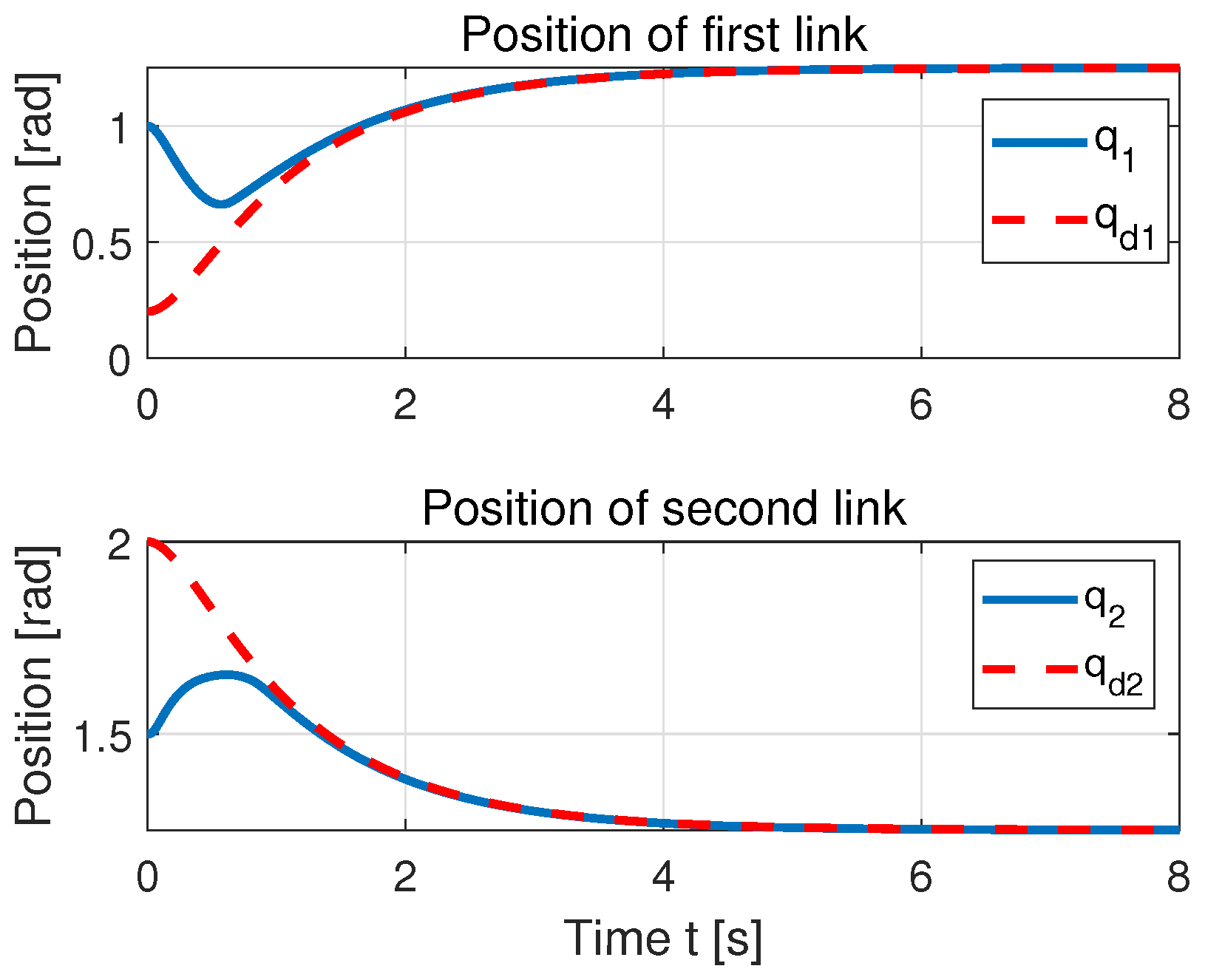
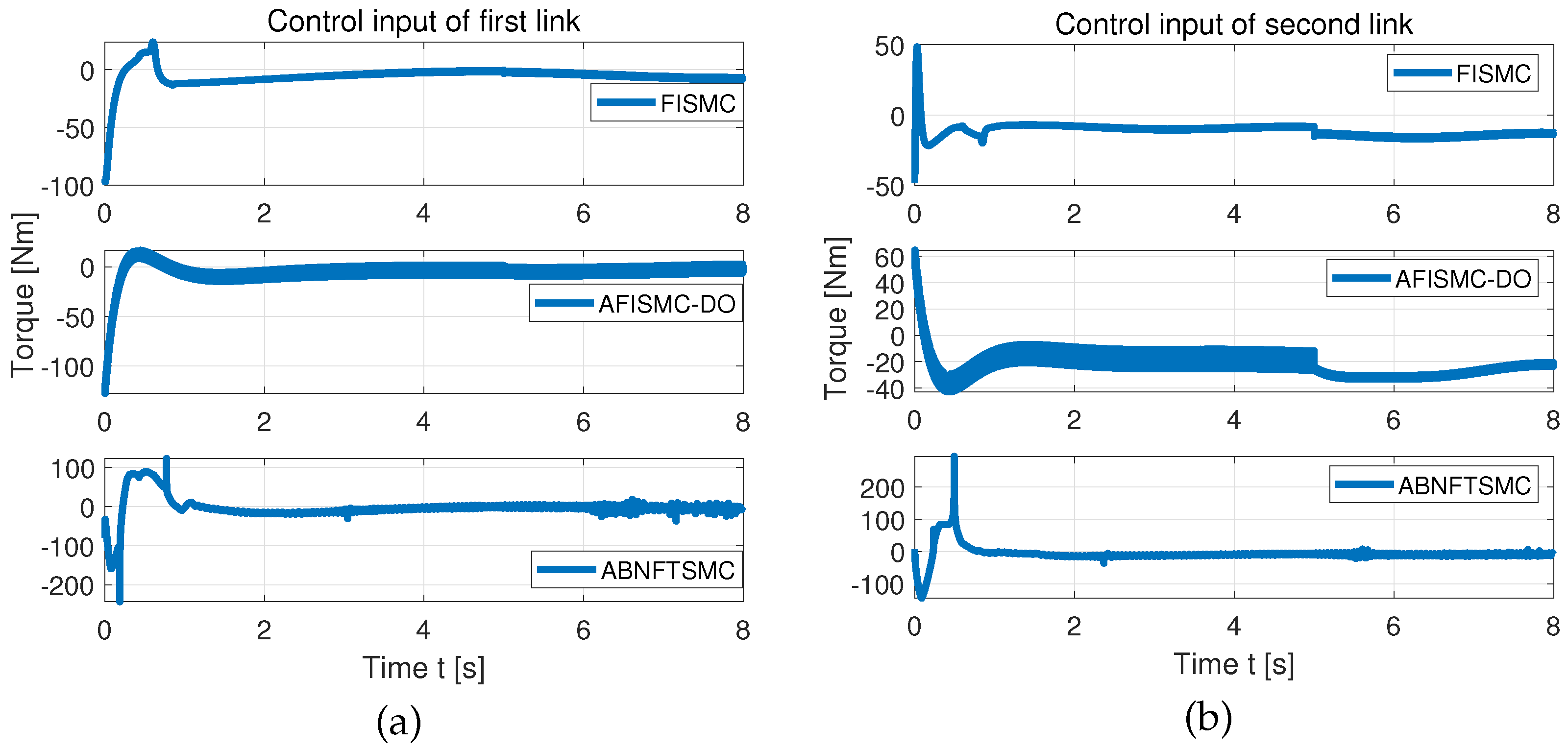
6. Simulation Results and Discussions

Consider the following robot manipulators

$$H\left(\xi \right)=\left[\begin{array}{cc}{F}_1+2F_{2}cos\left({\xi }_2\right)& F_3+F_{2}cos\left({\xi }_2\right)\\ F_3+F_{2}cos\left({\xi }_2\right)& F_4\end{array}\right]$$

(65)

$$K(\xi ,\dot{\xi })=\left[\begin{array}{cc}-F_{2}sin\left({\xi }_2\right){\dot{\xi }}_1& -2F_{2}sin\left({\xi }_2\right){\dot{\xi }}_1\\ 0& F_{2}sin\left({\xi }_2\right){\dot{\xi }}_2\end{array}\right]$$

(66)

$$G\left(\xi \right)=\left[\begin{array}{c}{F}_{5}cos\left({\xi }_1\right)+F_{6}cos({\xi }_1+{\xi }_2)\\ F_{6}cos({\xi }_1+{\xi }_2)\end{array}\right]$$

(67)

where

$$\begin{array}{c}{F}_1=\left(m_{s1}+m_{s2}\right)l_{s1}+m_{s2}{l}_{s2}^2+J_{s1},F_2=m_{s2}{l}_{s1}{l}_{s2},F_3=m_{s2}{l}_{s2}^2\\ F_4=F_3+J_{s2},F_5=\left(m_{s1}+m_{s2}\right)l_{s1}{g}_s,F_6=m_{s2}{l}_{s2}{g}_s\end{array}$$

(68)

The parameters of (66)–(69) are summarized as: $m_{s1}=0.5\mathrm{kg}$, $m_{s2}=1.5\mathrm{kg}$, $l_{s1}=1.0\mathrm{m}$, $l_{s2}=0.8\mathrm{m}$, $J_{s1}=J_{s2}=0.5\mathrm{kg}·\mathrm{m}$, and $g_s=9.8\mathrm{m}/\phantom{\mathrm{m}{\mathrm{s}}^2}{\mathrm{s}}^2$. The external disturbances $d={\left[d_1;d_2\right]}^T\in {\Re }^2$ are given as

$$d_1=2sin\left(t\right)+0.5sin\left(200\pi t\right);d_2=cos\left(2t\right)+0.5sin\left(200\pi t\right);$$

(69)

For the subsequent design, the initial conditions, such as the sampling period ($t_s$), the initial states ${\left[q{\left(0\right)}^T,\dot{q}{\left(0\right)}^T\right]}^T$, and the desired trajectories $q_d$, are as follows:

$$\begin{array}{c}{t}_s=1\mathrm{ms},{\left[\xi {\left(0\right)}^T,\dot{\xi }{\left(0\right)}^T\right]}^T={\left[1.0,1.0,0,0\right]}^T\\ {\xi }_d={\left[{\xi }_{d1},{\xi }_{d2}\right]}^T=\left[\begin{array}{c}1.25-1.4exp(-t)+0.35exp(-4t)\\ 1.25+exp(-t)-0.25exp(-4t)\end{array}\right]\end{array}$$

(70)

In the simulation comparisons, $\mathrm{{\rm Y}}$, as defined by (6), is

$$\mathrm{{\rm Y}}=\left\{\begin{array}{c}{I}_{2\times 2},t<8\mathrm{s}\hfill \\ \mathrm{diag}\left\{0.7+0.01sin\left(10t\right),0.65\right\}t\ge 8\mathrm{s}\hfill \end{array}\right.$$

(71)

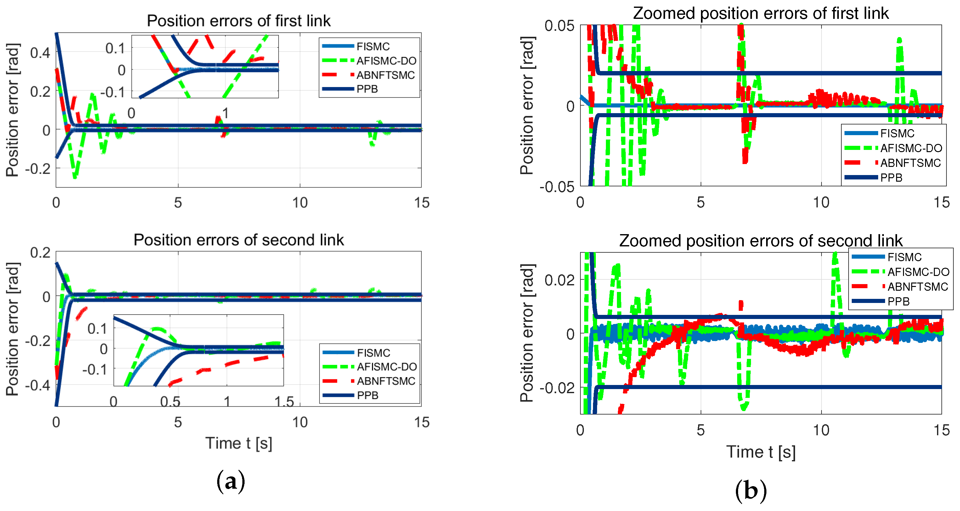
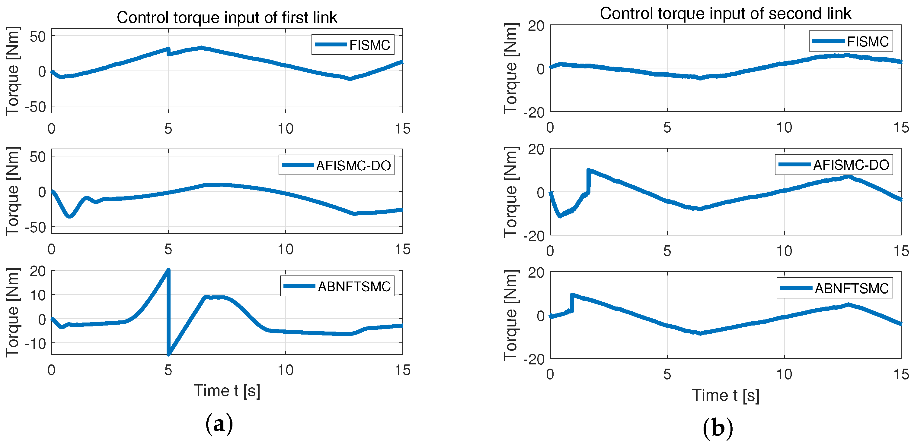
6.1. Tracking Performance Compared with AFISMC-DO and ABNFTSMC

The proposed FISMC can be compared with AFISMC-DO [45] and ABNFTSMC [48] for verifying the advanced tracking performance.

AFISMC-DO [48] is

$$u={\tau }_0+{\tau }_s$$

(72)

$${\tau }_0={\Lambda }^{-1}\left(-f(x_1,x_1)-{\widehat{W}}^T\Psi \left(Z\right)-\widehat{\Delta }+{\dot{\alpha }}_1-{\epsilon }_1-K_2{\epsilon }_2\right)$$

(73)

$${\tau }_s={\Lambda }^{-1}\left({\mu }_1{\left|\sigma \right|}^{1/\phantom{1/2}2}\mathrm{sign}\left(\sigma \right)+\xi \right)$$

(74)

$$x_1=\xi ,x_2=\dot{\xi },{\epsilon }_1=x_1-x_d$$

(75)

$${\epsilon }_2=x_2-{\alpha }_1,{\alpha }_1=-K_1{\epsilon }_1+{\dot{x}}_d$$

(76)

with $x_d={\xi }_d$ given by (9) and

$${\dot{\widehat{W}}}_i={\Gamma }_i\left[e_{2i}\Psi \left(Z\right)-2\gamma {\widehat{W}}_i\right]$$

(77)

$$\Lambda =H^{-1}\left(x_1\right),\dot{\xi }=k_s\left(t\right)\mathrm{sign}\left(\sigma \right)$$

(78)

$$\begin{array}{c}{\delta }_s\left(t\right)=k_s\left(t\right)-\frac{1}{{\nu }_1}\left|W_{eq}\left(t\right)\right|-{\nu }_0,{\nu }_0,{\nu }_1>0\\ {\dot{k}}_s\left(t\right)=-\left({\partial }_0+{\partial }_s\left(t\right)\right)\mathrm{sign}\left({\delta }_s\left(t\right)\right),{\partial }_0>0\\ {\dot{\partial }}_s\left(t\right)={\beta }_s\left|{\delta }_s\left(t\right)\right|,{\beta }_s>0\end{array}$$

(79)

and

$$\begin{array}{c}\sigma \left(t\right)=S\left(t\right)-S\left(0\right)-\int \left(\Lambda u_0+\prod \right)\mathrm{d}t\\ \prod =f\left(x_1,x_2\right)+{\widehat{W}}^T\Psi \left(Z\right)+\lambda \dot{e}-{\ddot{x}}_d+\widehat{\Delta }\\ f\left(x_1,x_2\right)=H^{-1}\left(x_1\right)(-K(x_1,x_2)x_2-G\left(x_1\right))\\ S=\dot{e}+\lambda e\\ \widehat{\Delta }\left(t\right)=p\left(t\right)+K_{o}S\\ \dot{p}\left(t\right)=-K_o\left(\widehat{\Gamma }\left(x_1,x_2,u,\dot{e},{\ddot{x}}_d\right)+\widehat{\Delta }\left(t\right)\right)\end{array}$$

(80)

where $\lambda >0$, ${\mu }_1>0$, ${\nu }_0>0$, ${\nu }_1>0$, ${\partial }_0>0$, and ${\beta }_s>0$, and $K_o,K_0,K_1\in {\Re }^{n\times n}$ are the constant matrices.

For ABNFTSMC [45], it follows that

$$u=\Xi \left(\dot{e}\right)H\left(x_1\right)\left(x_1\right)\left({\tau }_n\left(t\right)-{\tau }_{as}\left(t\right)\right)$$

(81)

with

$$\begin{array}{c}{u}_n\left(t\right)=-\Xi \left(\dot{e}\right)\left(f\left(x_1,x_2\right)-{\ddot{x}}_d\right)-\Psi (e,\dot{e})+{\alpha }_2-\int ({\xi }_2{\vartheta }_3+{\vartheta }_2)\\ {\dot{u}}_{as}\left(t\right)=\left(\widehat{\Lambda }+\zeta \right)\mathrm{sign}\left({\vartheta }_3\right)\end{array}$$

(82)

where

$$\begin{array}{c}\dot{\widehat{\Lambda }}=\left\{\begin{array}{c}0,\mathrm{if}\left|{\vartheta }_3\right|\le \epsilon \hfill \\ \frac{1}{\delta }\left|{\vartheta }_3\right|,\mathrm{if}\left|{\vartheta }_3\right|>\epsilon \hfill \end{array}\right.\\ {\vartheta }_1={\sigma }_1,{\vartheta }_2={\sigma }_2-{\alpha }_1,{\vartheta }_3={\sigma }_3-{\alpha }_2\end{array}$$

(83)

$$\begin{array}{c}{\sigma }_1=\int \left(\left(e+k_1\mathrm{Si}{\mathrm{g}}^{\lambda }\left(e\right)+k_1\mathrm{Si}{\mathrm{g}}^{p/\phantom{pq}q}\left(\dot{e}\right)\right)\right)\\ {\sigma }_2={\dot{\sigma }}_1,{\sigma }_3={\ddot{\sigma }}_1\end{array}$$

(84)

where $x_1=q$, e, and $\dot{e}$ are defined by (9), $f\left(x_1,x_2\right)$ is defined by (81), and $k_1$, $k_2$, $\lambda$, p, q, ${\xi }_1$, ${\xi }_2$, $\delta$, and $\epsilon$ stand for some positive constants.

Note that $H_0\left(\xi \right)$, $K_0(\xi ,\dot{\xi })$, and $G_0\left(\xi \right)$ replace $m_1$ and $m_2$ of (66)–(69) with $m_{s1}=0.4\mathrm{kg}$ and $m_{s1}=1.2\mathrm{kg}$. Further, $H_0$ of the proposed FISMC is defined by (24). The parameters of these controllers are given in

Table 1. Controller parameters selection.

Controllers	Parameters
FISMC	$\begin{array}{c}{\eta }_{01}=1.2,{\eta }_{02}=0.6,{\eta }_{\infty 1}={\eta }_{\infty 2}=0.002,l_1=2,l_2=2.2\\ r=0.5,\delta =0.1,{\lambda }_1=5,{\lambda }_2=7,{\gamma }_1=0.5,{\upsilon }_1=1.1,{\upsilon }_2=0.1\\ b=0.2,c_0=2.8,c_1=2.2,z_1=0.2,z_2=0.09,S_0=0.005\end{array}$
ABNFTSMC [45]	$\begin{array}{c}{k}_1=1,k_2=0.5,{\lambda }_1=1.4,p=9,q=7,{\xi }_1=1,{\xi }_2=0.5\\ {\xi }_3=0.1,\delta =0.5,\epsilon =0.01,m_1=m_2=m_3=20\end{array}$
AFISMC-DO [48]	$\begin{array}{c}\lambda =5,{\mu }_1=10,{\upsilon }_0=3,{\upsilon }_1=2,{\partial }_0=3,{\beta }_s=5\\ K_o=5I_n,K_1=K_2=K_o,\Gamma =2,\gamma =1\end{array}$

.

Figure 2 gives the position tracking of the proposed FISMC. Figure 3 and Figure 4 represent the position and velocity tracking errors with their plots of FISMC, ABNFTSMC, and AFISMC-DO, while Figure 5 depicts the control torque input of FISMC, ABNFTSMC, and AFISMC-DO. As seen in Figure 3b and Figure 4b, the proposed FISMC is still stable at the prescribed performance bound (PPB). By contrast, the other controllers cannot guarantee the prescribed tracking performance for all times. On the other hand, the proposed FISMC reveals a better steady-state tracking precision than AFISMC-DO and ABNFTSMC. In addition, the steady-state tracking errors always oscillate around zero in Figure 3 and Figure 4. The key point of such favorable results is that the proposed FISMC eliminates the reaching phase of the conventional sliding mode controls and combines the prescribed tracking technique in order to acquire the prescribed tracking performance. Moreover, such favorable tracking results do not utilize the excessive control efforts of the AFISMC-DO and ABNFTSMC.

To further give a quantitative comparison between the proposed FISMC and the other approaches, the following indicators have been compared: the position and velocity tracking precision, and the control efforts after $3s$ at the very beginning of the simulation comparison.

$$P_e=\sqrt{\frac{1}{N}\sum _{i=1}^n{∥\epsilon \left(n\right)∥}^2}$$

(85)

$$V_e=\sqrt{\frac{1}{N}\sum _{i=1}^n{∥\dot{\epsilon }\left(n\right)∥}^2}$$

(86)

$$u_e=\sqrt{\frac{1}{N}\sum _{i=1}^n{∥u\left(n\right)∥}^2}$$

(87)

where N is the total sampling number, and $u\left(n\right)$, $\epsilon \left(n\right)$, and $\dot{\epsilon }\left(n\right)$ are the sampling of the control input, position, and velocity tracking errors, respectively. These three indicators are illustrated in

Table 2. Comparison of control performance.

Controller	${\mathit{P}}_{\mathit{e}}$	${\mathit{V}}_{\mathit{e}}$	${\mathit{u}}_{\mathit{e}}$
FISMC	$2.5\times {10}^{-3}$	$3.7\times {10}^{-3}$	$13.17$
ABNFTSMC	$9.61\times {10}^{-2}$	$7.82\times {10}^{-2}$	$15.61$
AFISMC-DO	$1.59\times {10}^{-2}$	$1.17\times {10}^{-2}$	$14.02$

.

As seen in Table 2, the proposed FISMC has higher position and velocity tracking precision ($P_e$ and $V_e$) compared with ABNFTSMC and AFISMC-DO. Moreover, such favorable results can be acquired from a lower control torque input $u_e$. The reasons behind this can be summarized as follows: (i) the proposed approach removes the reaching phase of the sliding mode control; (ii) the prescribed tracking performance is guaranteed by the proposed FISMC; (iii) a simple control structure can be utilized to obtain advanced tracking performance.

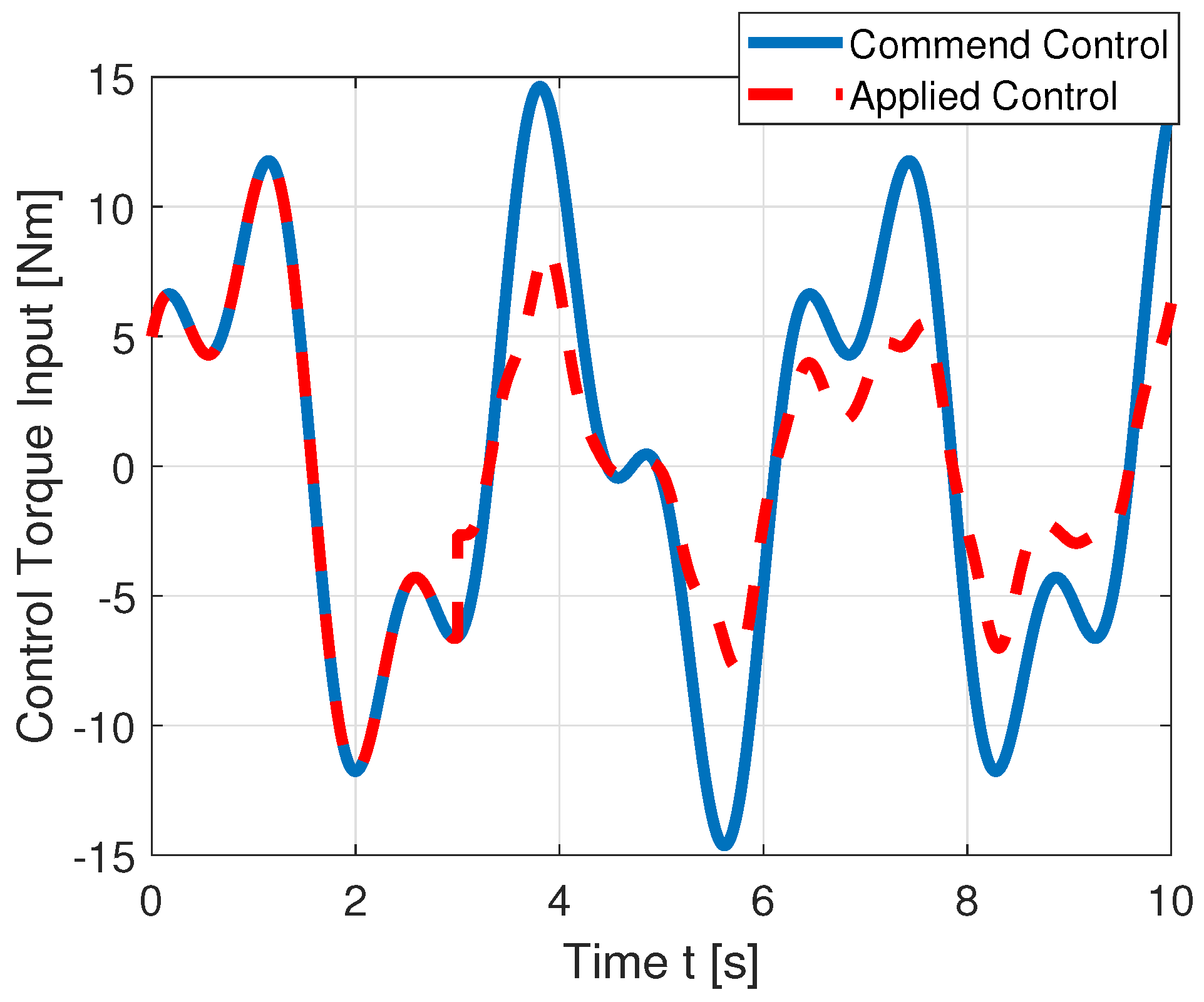
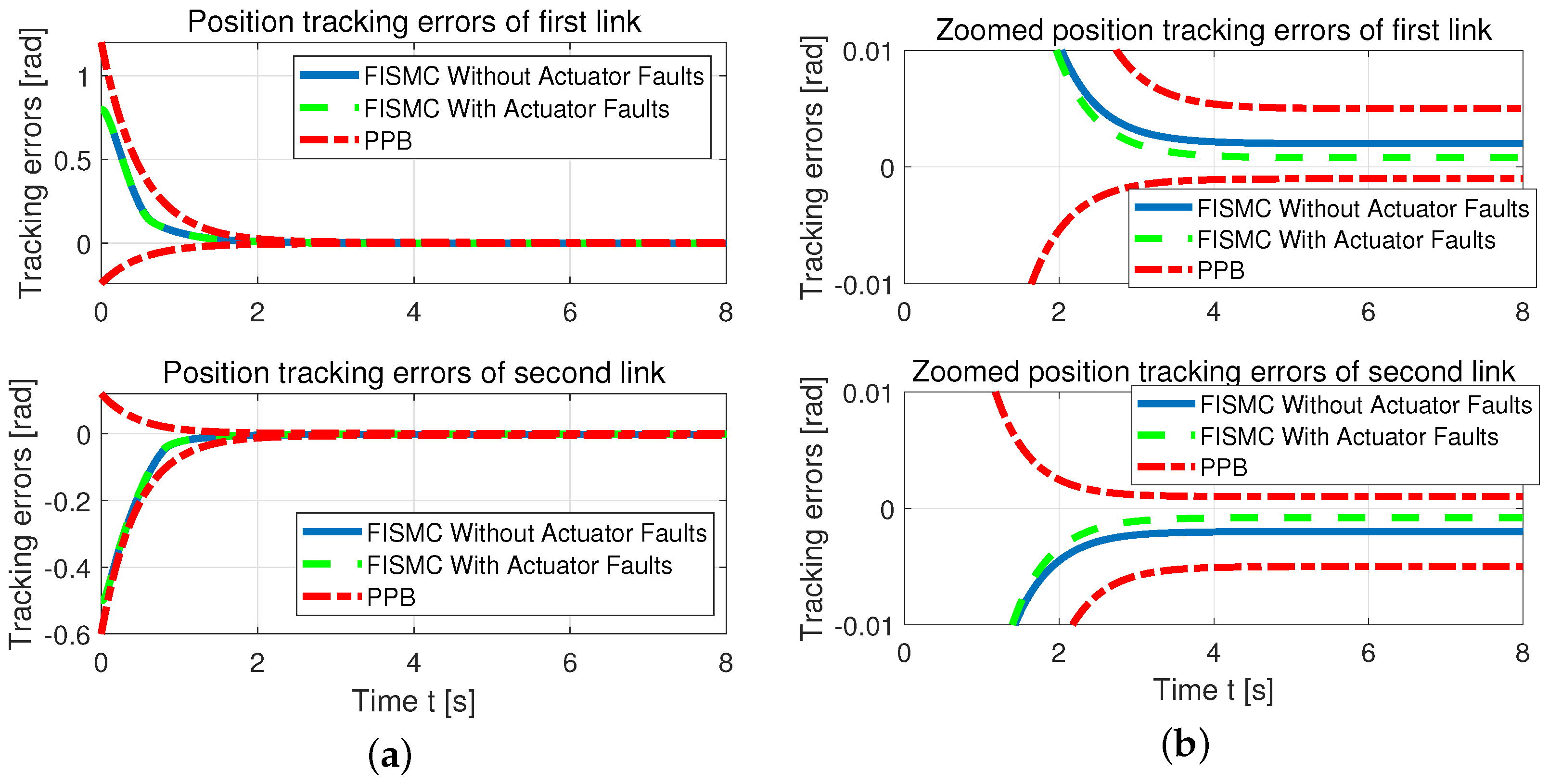
6.2. Tracking Performance with/without Actuator Faults

In order to show the effect of the actuator faults on the tracking performance, in this section we perform several simulations of the proposed FISMC with/without the actuator faults. In this simulation, the simulation conditions and parameters are same as in Section 6.1, given by Figure 3, Figure 4 and Figure 5.

Figure 6 depicts the position tracking performance of FISMC with/without actuator faults, while Figure 7 gives the control torque input of FISMC with/without actuator faults. In light of Figure 7b, the proposed approach reveals higher steady-state tracking precision for uncertain robot manipulators with actuator faults compared to those without actuator faults. In addition, the favorable results of the proposed approach do not utilize excessive control efforts for uncertain robot manipulators compared to those with actuator faults. As a result, the proposed approach demonstrates the actuator faults.

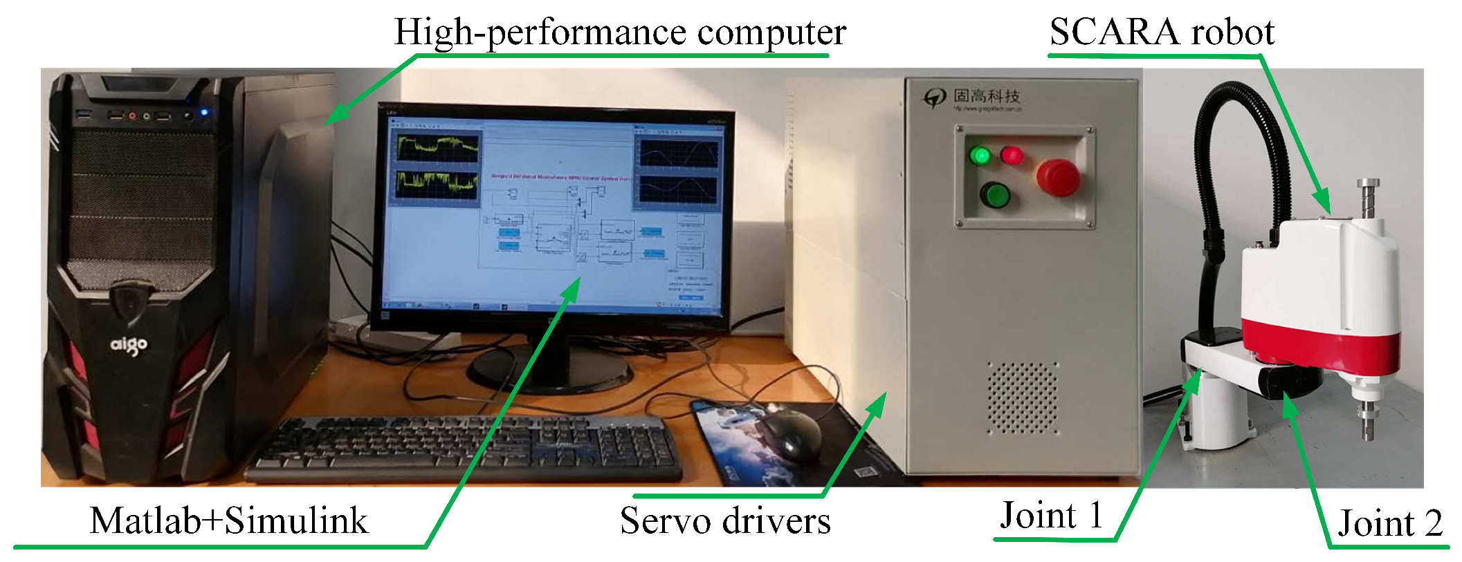
7. Experimental Comparison

In this section, the advanced tracking performance is accomplished by the SCARA robot platform, shown in Figure 8. In this experimental platform, the maximum control torques of two joints are given as ${\left[\pm 51.2\pm 16\right]}^T\left(\mathrm{Nm}\right)$, with the harmonic reduction ratios as 1:80 and 1:50, respectively. The torques can be acquired by the higher performance computer of the Simulink of Matlab 2012b. The parameters of FISMC, ABNFTSMC, AFISMC-DO are introduced in Table 2.

For the experimental comparisons, the sample period is selected as $t_s=2\mathrm{s}$. The initial states are $q=[0;0]\left(\mathrm{rad}\right)$, and the desired trajectories are

$$q_d={\left[-\frac{\pi }{10}sin\left(\frac{t}{2}+\frac{\pi }{2}\right),\frac{\pi }{10}sin\left(\frac{t}{2}+\frac{\pi }{2}\right)\right]}^T$$

(88)

To ensure fair conditions, the same health conditions (71) are used in the following experimental comparisons for robot manipulators.

Figure 9 gives the position tracking results of FISMC by utilizing the experimental platform. Figure 10 represents the position tracking errors of FISMC, AFISMC-DO, and ABNFTSMC with their zoomed plots, while Figure 11 denotes the control torque input. The joint position can tracks the desired trajectory correctly in Figure 9. As seen in Figure 10, the proposed FISMC shows higher steady-state tracking precision than ABNFTSMC and AFISMC-DO; meanwhile, the steady-state tracking errors of the proposed FISMC are still stable at the PPB. Moreover, the steady-state precision of ABNFTSMC and AFISMC-DO cannot be restrained by the PPB. In view of the above experimental results, the proposed FISMC has a fast transient rate and high steady-state tracking precision compared to ABNFTSMC and AFISMC-DO. Such favorable results of the proposed FISMC do not utilize an excessive control input.

8. Conclusions

In this paper, an FTC is developed for robot manipulators, which has several advantages such as strong robustness, chattering-restraining, a high steady-state tracking precision, prescribed performance, and a simple control structure. The simulation and experimental comparisons verify the advanced tracking performance with high steady-state tracking precision compared with other controllers in Figure 1, Figure 2, Figure 3, Figure 4, Figure 5 and Figure 6. Moreover, the tracking performance in transient and steady states has been guaranteed for acquiring the prescribed performance. Moreover, such favorable performance does not utilize an excessive control input torque. The reason behind this is that the proposed approach constructs an integral sliding manifold with prescribed performance, and then the fault-tolerant tracking control is developed for robot manipulators subject to uncertainties and actuator faults. So, the developed control strategy offers an alternative approach for the formulation of robot manipulators for the fault-tolerant tracking problem.

References

1. Yu, H.; Shen, J.H.; Joos, K.M.; Simaan, N. Calibration and integration of b-mode optical coherence tomography for assistive control in robotic microsurgery. IEEE/ASME Trans. Mechatron. 2016, 21, 2613–2623. [Google Scholar] [CrossRef]
2. Xiao, B.; Yin, S.; Kaynak, O. Tracking control of robotic manipulators with uncertain kinematics and dynamics. IEEE Trans. Ind. Electron. 2016, 63, 6439–6449. [Google Scholar] [CrossRef]
3. Lee, J.Y.; Jin, M.; Chang, P.H. Variable PID gain tuning method using backstepping control with time-delay estimation and nonlinear damping. IEEE Trans. Ind. Electron. 2014, 61, 6975–6985. [Google Scholar] [CrossRef]
4. Lee, J.; Chang, P.H.; Jamisola, R.S. Relative impedance control for dual-arm robots performing asymmetric bimanual tasks. IEEE Trans. Ind. Electron. 2013, 61, 3786–3796. [Google Scholar] [CrossRef]
5. Islam, S.; Liu, X.P. Robust sliding mode control for robot manipulators. IEEE Trans. Ind. Electron. 2010, 58, 2444–2453. [Google Scholar] [CrossRef]
6. Jie, W.; Yudong, Z.; Yulong, B.; Kim, H.H.; Lee, M.C. Trajectory tracking control using fractional-order terminal sliding mode control with sliding perturbation observer for a 7-DOF robot manipulator. IEEE/ASME Trans. Mechatron. 2020, 25, 1886–1893. [Google Scholar] [CrossRef]
7. Jin, M.; Kang, S.H.; Chang, P.H.; Lee, J. Robust control of robot manipulators using inclusive and enhanced time delay control. IEEE/ASME Trans. Mechatron. 2017, 22, 2141–2152. [Google Scholar] [CrossRef]
8. Van, M. An enhanced robust fault tolerant control based on an adaptive fuzzy PID-nonsingular fast terminal sliding mode control for uncertain nonlinear systems. IEEE/ASME Trans. Mechatron. 2018, 23, 1362–1371. [Google Scholar] [CrossRef]
9. Nguyen, N.P.; Mung, N.X.; Thanh Ha, L.N.N.; Huynh, T.T.; Hong, S.K. Finite-time attitude fault tolerant control of quadcopter system via neural networks. Mathematics 2020, 8, 1541. [Google Scholar] [CrossRef]
10. Li, Y.; Liang, H. Robust finite-time control algorithm based on dynamic sliding mode for satellite attitude maneuver. Mathematics 2022, 10, 111. [Google Scholar] [CrossRef]
11. Gang, C.; Wang, P.; Zhenyu, W.; Jiajun, T.; Huosheng, H.; Donghai, W.; Hao, C.; Lvyuan, Z. Modeling of swimming posture dynamics for a beaver-like robot. Ocean Eng. 2019, 29, 1396–1417. [Google Scholar]
12. Chen, G.; Zhao, Z.; Wang, Z.; Tu, J.; Hu, H. Swimming modeling and performance optimization of a fish-inspired underwater vehicle (FIUV). Ocean Eng. 2023, 271, 113748. [Google Scholar] [CrossRef]
13. Shen, G.; Xia, Y.; Ma, D.; Zhang, J. Adaptive sliding-mode control for Mars entry trajectory tracking with finite-time convergence. Int. J. Robust Nonlinear Control 2019, 29, 1249–1264. [Google Scholar] [CrossRef]
14. Ma, Z.; Huang, P. Adaptive neural-network controller for an uncertain rigid manipulator with input saturation and full-order state constraint. IEEE Trans. Cyber. 2020, 52, 2907–2915. [Google Scholar] [CrossRef] [PubMed]
15. Liu, L.; Zhang, L.; Hou, Y.; Tang, D.; Liu, H. Implementation of Adaptive Fault-Tolerant Tracking Control for Robot Manipulators with Integral Sliding Mode; Wiley Online Library: Hoboken, NJ, USA, 2023. [Google Scholar]
16. Ji, P.; Li, C.; Ma, F. Sliding Mode Control of Manipulator Based on Improved Reaching Law and Sliding Surface. Mathematics 2022, 10, 1935. [Google Scholar] [CrossRef]
17. Najafi, A.; Vu, M.T.; Mobayen, S.; Asad, J.H.; Fekih, A. Adaptive barrier fast terminal sliding mode actuator fault tolerant control approach for quadrotor UAVs. Mathematics 2022, 10, 3009. [Google Scholar] [CrossRef]
18. Slotine, J.J.E.; Li, W. Applied Nonlinear Control; Prentice Hall: Englewood Cliffs, NJ, USA, 1991; Volume 199. [Google Scholar]
19. Feng, Y.; Yu, X.; Man, Z. Non-singular terminal sliding mode control of rigid manipulators. Automatica 2002, 38, 2159–2167. [Google Scholar] [CrossRef]
20. Yu, S.; Yu, X.; Shirinzadeh, B.; Man, Z. Continuous finite-time control for robotic manipulators with terminal sliding mode. Automatica 2005, 41, 1957–1964. [Google Scholar] [CrossRef]
21. Alipour, M.; Malekzadeh, M.; Ariaei, A. Practical fractional-order nonsingular terminal sliding mode control of spacecraft. ISA Trans. 2022, 128, 162–173. [Google Scholar] [CrossRef]
22. Wang, Y.; Li, B.; Yan, F.; Chen, B. Practical adaptive fractional-order nonsingular terminal sliding mode control for a cable-driven manipulator. Int. J. Robust Nonlinear Control 2019, 29, 1396–1417. [Google Scholar] [CrossRef]
23. Polyakov, A. Nonlinear feedback design for fixed-time stabilization of linear control systems. IEEE Trans. Autom. Control 2011, 57, 2106–2110. [Google Scholar] [CrossRef]
24. Polyakov, A.; Efimov, D.; Perruquetti, W. Robust stabilization of MIMO systems in finite/fixed time. Int. J. Robust Nonlinear Control 2016, 26, 69–90. [Google Scholar] [CrossRef]
25. Cao, W.J.; Xu, J.X. Nonlinear integral-type sliding surface for both matched and unmatched uncertain systems. IEEE Trans. Autom. Control 2004, 49, 1355–1360. [Google Scholar] [CrossRef]
26. Wang, Y.; Xia, Y.; Li, H.; Zhou, P. A new integral sliding mode design method for nonlinear stochastic systems. Automatica 2018, 90, 304–309. [Google Scholar] [CrossRef]
27. Niu, Y.; Ho, D.W.; Lam, J. Robust integral sliding mode control for uncertain stochastic systems with time-varying delay. Automatica 2005, 41, 873–880. [Google Scholar] [CrossRef]
28. Jiang, B.; Karimi, H.R.; Kao, Y.; Gao, C. A novel robust fuzzy integral sliding mode control for nonlinear semi-Markovian jump T–S fuzzy systems. IEEE Trans. Fuzzy Syst. 2018, 26, 3594–3604. [Google Scholar] [CrossRef]
29. Shao, K. Nested adaptive integral terminal sliding mode control for high-order uncertain nonlinear systems. Int. J. Robust Nonlinear Control 2021, 31, 6668–6680. [Google Scholar] [CrossRef]
30. Li, J.; Zhai, D. A descriptor regular form-based approach to observer-based integral sliding mode controller design. Int. J. Robust Nonlinear Control 2021, 31, 5134–5148. [Google Scholar] [CrossRef]
31. Lee, J.; Chang, P.H.; Jin, M. Adaptive integral sliding mode control with time-delay estimation for robot manipulators. IEEE Trans. Ind. Electron. 2017, 64, 6796–6804. [Google Scholar] [CrossRef]
32. Ferrara, A.; Incremona, G.P. Design of an integral suboptimal second-order sliding mode controller for the robust motion control of robot manipulators. IEEE Trans. Control Syst. Technol. 2015, 23, 2316–2325. [Google Scholar] [CrossRef]
33. Qin, J.; Ma, Q.; Gao, H.; Zheng, W.X. Fault-tolerant cooperative tracking control via integral sliding mode control technique. IEEE/ASME Trans. Mechatron. 2017, 23, 342–351. [Google Scholar] [CrossRef]
34. Van, M.; Ge, S.S.; Ren, H. Robust fault-tolerant control for a class of second-order nonlinear systems using an adaptive third-order sliding mode control. IEEE Trans. Syst. Man Cyber. Syst. 2016, 47, 221–228. [Google Scholar] [CrossRef]
35. Huang, H.; He, W.; Li, J.; Xu, B.; Yang, C.; Zhang, W. Disturbance observer-based fault-tolerant control for robotic systems with guaranteed prescribed performance. IEEE Trans. Cyber. 2020, 52, 772–783. [Google Scholar] [CrossRef] [PubMed]
36. Van, M.; Kang, H.J.; Suh, Y.S.; Shin, K.S. A robust fault diagnosis and accommodation scheme for robot manipulators. Int. J. Control Autom. Syst. 2013, 11, 377–388. [Google Scholar] [CrossRef]
37. He, X.; Wang, Z.; Qin, L.; Zhou, D. Active fault-tolerant control for an internet-based networked three-tank system. IEEE Trans. Control Syst. Tech. 2016, 24, 2150–2157. [Google Scholar] [CrossRef]
38. Zhang, L.; Liu, H.; Tang, D.; Hou, Y.; Wang, Y. Adaptive fixed-time fault-tolerant tracking control and its application for robot manipulators. IEEE Trans. Ind. Electron. 2021, 69, 2956–2966. [Google Scholar] [CrossRef]
39. Karayiannidis, Y.; Doulgeri, Z. Model-free robot joint position regulation and tracking with prescribed performance guarantees. Robo. Autonom. Syst. 2012, 60, 214–226. [Google Scholar] [CrossRef]
40. Bechlioulis, C.P.; Rovithakis, G.A. Robust adaptive control of feedback linearizable MIMO nonlinear systems with prescribed performance. IEEE Trans. Autom. Control 2008, 53, 2090–2099. [Google Scholar] [CrossRef]
41. Bechlioulis, C.P.; Rovithakis, G.A. Prescribed performance adaptive control for multi-input multi-output affine in the control nonlinear systems. IEEE Trans. Autom. Control 2010, 55, 1220–1226. [Google Scholar] [CrossRef]
42. Jing, Y.; Liu, Y.; Zhou, S. Prescribed performance finite-time tracking control for uncertain nonlinear systems. J. Syst. Sci. Complex. 2019, 32, 803–817. [Google Scholar] [CrossRef]
43. Yang, P.; Su, Y. Proximate fixed-time prescribed performance tracking control of uncertain robot manipulators. IEEE/ASME Trans. Mechatron. 2021, 27, 3275–3285. [Google Scholar] [CrossRef]
44. Hao, L.Y.; Park, J.H.; Ye, D. Integral sliding mode fault-tolerant control for uncertain linear systems over networks with signals quantization. IEEE Trans. Neural Netw. Learn. Syst. 2016, 28, 2088–2100. [Google Scholar] [CrossRef] [PubMed]
45. Van, M.; Ge, S.S. Adaptive fuzzy integral sliding-mode control for robust fault-tolerant control of robot manipulators with disturbance observer. IEEE Trans. Fuzzy Syst. 2020, 29, 1284–1296. [Google Scholar] [CrossRef]
46. Zhang, L.; Liu, L.; Wang, Z.; Xia, Y. Continuous finite-time control for uncertain robot manipulators with integral sliding mode. IET Control Theory Appl. 2018, 12, 1621–1627. [Google Scholar] [CrossRef]
47. Zhu, W.H. Comments on “Robust tracking control for rigid robotic manipulators”. IEEE Trans. Autom. Control 2000, 45, 1577–1580. [Google Scholar] [CrossRef]
48. Van, M.; Mavrovouniotis, M.; Ge, S.S. An adaptive backstepping nonsingular fast terminal sliding mode control for robust fault tolerant control of robot manipulators. IEEE Trans. Syst. Man. Cybern. Syst. 2018, 49, 1448–1458. [Google Scholar] [CrossRef]
49. Sciavicco, L.; Siciliano, B. Modelling and Control of Robot Manipulators; Springer Science & Business Media: Berlin/Heidelberg, Germany, 2001. [Google Scholar]
Figure 1. Control torque input with actuator health condition.
Mathematics 11 02430 g001
Figure 2. Position tracking of FISMC.
Mathematics 11 02430 g002
Figure 3. (a) Position tracking errors of FISMC, AFISMC-DO, and ABNFTSMC; (b) zoomed position tracking errors of FISMC, AFISMC-DO, and ABNFTSMC.
Mathematics 11 02430 g003
Figure 4. (a) Velocity tracking errors of FISMC, AFISMC-DO, and ABNFTSMC; (b) zoomed velocity tracking errors of FISMC, AFISMC-DO, and ABNFTSMC.
Mathematics 11 02430 g004
Figure 5. (a) Control torque input of first link; (b) control torque input of second link.
Mathematics 11 02430 g005
Figure 6. (a) Position tracking errors of FISMC with/without actuator faults; (b) zoomed position tracking errors of FISMC with/without actuator faults.
Mathematics 11 02430 g006
Figure 7. (a) Control torque input of first link for FISMC with/without actuator faults; (b) control torque input of second link for FISMC with/without actuator faults.
Mathematics 11 02430 g007
Figure 8. The experimental robot setup.
Mathematics 11 02430 g008
Figure 9. The position tracking of FISMC.
Mathematics 11 02430 g009
Figure 10. (a) Position tracking errors of FISMC, AFISMC-DO, and ABNFTSMC; (b) zoomed position tracking errors of FISMC, AFISMC-DO, and ABNFTSMC.
Mathematics 11 02430 g010
Figure 11. (a) Control torque input of first link; (b) control torque input of second link.
Mathematics 11 02430 g011