TRX Cryptocurrency Profit and Transaction Success Rate Prediction Using Whale Optimization-Based Ensemble Learning Framework

Abstract

TRON is a decentralized digital platform that provides a reliable way to transact in cryptocurrencies within a decentralized ecosystem. Thanks to its success, TRON’s native token, TRX, has been widely adopted by a large audience. To facilitate easy management of digital assets with TRON Wallet, users can securely store and manage their digital assets with ease. Our goal is first to develop a methodology to predict the future price using regression and then move on to build an effective classifier to predict whether a profit or loss is made the next day and then make a prediction of the transaction success rate. Our framework is capable of predicting whether there will be a profit in the future based on price prediction and forecasting results using regressors such as XGBoost, LightGBM, and CatBoost with $R^2$ values of 0.9820, 0.9825 and 0.9858, respectively. In this work, an ensemble-based stacking classifier with the Whale optimization approach has been proposed which achieves the highest accuracy of 89.05 percent to predict if there will be a profit or loss the next day and an accuracy of 98.88 percent of TRX transaction success rate prediction which is higher than accuracies obtained by standard machine learning models. An effective framework will be useful for better decision-making and management of risks in a cryptocurrency.

1. Introduction

Blockchain technology has emerged as a game-changer in the wake of the success of Bitcoin and other cryptocurrencies. Decentralized application developers tend to instead focus on finding a solution that best meets their needs and the needs of their decentralized applications market rather than developing a new blockchain platform from scratch as the number of existing ones grows. Decentralization-based technologies guarantees the ownership and transferability of digital financial assets to a certain extent. The upsurge in market value and popularity of cryptocurrencies raises several global issues and concerns for business and industrial economics. Distributed ledger has gained traction over the years and refers to the technological infrastructure and protocols to meet the very objectives of transparency and traceability. For each secure transaction, a separate secure location has to be maintained over the internet by the participants, who are essentially the users of the distributed ledger technology. Blockchain makes it possible to maintain a widely dispersed network through cooperative efforts to establish mechanisms for coordination, communication, and motivation [1]. The term “blockchain finance” refers to how this technology has been implemented. This has given rise to several digital platforms, such as TRON, which has its own digital coin, called the TRX coin. The usage of blockchain technology in the finance sector reduces costs and improves service quality in a safe and flexible manner [2]. The Blockchain distributed database is nearly impossible to alter, whereas traditional credit models rely on third parties to process payment information. As a result of peer-to-peer innovation and decentralization in the financial sector, there has been rapid global expansion and a trustworthy database.

The basis of a blockchain is an immutable, tamper-proof chain of linked blocks. Sets are recorded in each block, and the metadata are associated with a transaction. It was launched as a peer-to-peer currency exchange system. Blockchain topologies act as a critical parameter in developing a blockchain application by classifying the nodes that will be a part of it. Permissioned, private, and hybrid blockchain systems are the most recent subdivisions of blockchain technology [3,4]. Transactions on the Blockchain have the same effect on both parties; each node has its ledger [5]. The role of digital currency tokens, often referred to as crypto-tokens, have a unique role in transforming the way people make transactions over the web. This has become more useful since the introduction of the first crypto-currencies such as Bitcoin [6] and Ethereum [7] that have nodes that can generate the next valid block without consensus [8]. TRX serves a similar function fundamentally, to make safe and secure transactions digitally. The TRON Protocol, one of the biggest operating systems based on blockchain, provides scalability, availability, and high throughput for the Decentralized Applications (Daps) in the TRON environment [9,10]. TRON Protobuf is a serialization mechanism for structured data, similar to JSON or XML but significantly faster and smaller [11]. A custom-built blockchain network, such as TRON, may be more efficient, convenient, secure, and stable for millions of global developers [12]. For now, it is impossible to predict how high TRON (TRX Token) will rise. The primary goal of the TRON network is to decentralize the distribution and content creation industry, which has been criticized for censorship and revenue distribution unfairly. Without a doubt, as individuals, it is our own responsibility to act ethically when it comes to digital media and always take responsibility for the content we post online or on any digital media platform. Additionally, TRON provides a few other tools to help ensure more democratic content creation. TRON was reasonably conceived as an innovative solution to address robust scalability issues and appears to be like its competitors on the surface. All of them could just as easily create Daps that further motivate the increase in the adoption of TRON. Quite a few of them already have. That being said, TRON still has the potential to succeed better in this market if its adoption increases over time. It is possible that the growing importance of interoperability in the blockchain industry will help TRON maintain its position as one of the leading networks for the distribution of original digital content. TRON’s unique selling point is that anyone, anywhere, with an internet connection, can access data on the network. Several researchers have made useful attempts in the blockchain and cryptocurrency sphere leading up to the present, where these works validate the usefulness of various Artificial Intelligence techniques in the technology. Very few attempts, if any, have been made to study TRON as a cryptocurrency by applying Artificial Intelligence to predict profit the next day, prices in the future, and address transaction success and failure rates. The scope and flexibility of the research and a framework that can be applied when analyzing digital tokens, as well as other cryptocurrencies having a relatively good standing in the market.

The followings are highlights of the contributions of the paper:

• We checked the potential capabilities of regression models such as Catboost, Xgboost and Light GBM for predicting the future price of cryptocurrencies.
• We have proposed classification models for TRX transaction success rate powered by machine learning techniques.
• Finally, we have estimated the earnings from the profit made by the TRX tokens.

The rest of this paper is organized as follows: Section 2 is about the literature review pertaining to blockchain technology and cryptocurrency price prediction. Section 3 is about the dataset, visualizations and discussion about the detailed methodology involved in this research. Section 4 exhibits the experimental results obtained by individual classifiers as well as ensemble methods along with its analysis. The paper is concluded in Section 5.

2. Literature Survey

The market value of the TRX coin is closely tied to the broader applications of blockchain technology, and to make accurate price predictions for specific coins, it is crucial to study related research findings and recent approaches. Factors such as market sentiment, regulatory changes, and technological advancements can greatly affect the value of TRX. It is also well argued that the price of a particular decentralized currency, just like TRX, follow other similar cryptocurrency on market trends. The reasons may be that it is seen as an asset, just like equity in the public market shareholdings (stock market), and is heavily dependent on market sentiments and the technology behind it. Therefore, we discuss these separately along with the literature on cryptocurrency price predictions.

2.1. Literature on the Scope of Cryptocurrencies and the Blockchain Technology

In this section, we survey several papers related to our work and group them accordingly. The key findings, mechanisms, and objectives are discussed. Vergne et al. [13], provide insights on Blockchain, machine learning (ML), and the future of digital platforms: centralized vs. distributed organizations. Sabry et al. [14] provide an overview of how artificial intelligence (AI) is being used to to find solutions for problems associated with cryptocurrency, including the inability of humans to keep up with the sheer volume of daily transactions, trades, and news. Recent studies in this field are discussed, with comparisons between them regarding methodology and data sets. It also calls attention to several improvement opportunities and research gaps. On the same lines, Bhutta et al. [15] explored the history, design, and safety of blockchain technology. Tanwar et al. [16] reviewed interdependent price prediction schemes for cryptocurrencies using deep learning techniques and predicted the value of cryptocurrencies using deep learning and their dependent relationships. They propose a hybrid model based on a deep learning approach to estimate the price of Litecoin and Zcash and the suggested model has been successfully trained and tested on industry-standard data sets, allowing immediate use in real-world settings. These cryptocurrencies are similar to TRX in the context of their relative market sizes. Šťastný et al. [17], looked at dynamic time warping and machine learning, they create a model and cluster the top 30 cryptocurrency prices. Their elaboration on how AI is influencing cryptocurrency is useful to understand the essentials of price predictions. Godsiff et al. [18], in their work, ‘Bitcoin: Bubble or Blockchain’, where agent and multi-agent systems are discussed; applications and new technologies and provided a brief, comprehensive overview of the cryptocurrency that is managed by a distributed multi-agent system (DAS). Along with this, Bachani et al. [19] discuss different blockchain platforms that use the Delegated proof of stake (DPoS) consensus algorithm, including Tron, and explain the specific features and properties of each platform, such as the number of validators (or delegates), block creation time, block reward, and how validators are chosen. It is, therefore, safe to say that, given the traction, the cryptocurrencies have gained, Blockchain will see increased adoption as a technology and have a very strong technological background. TRON, therefore, relies on some of the most innovative technologies ever developed and the TRX token has great potential in this regard.

2.2. Literature on Related Applications of Blockchain Technology

Alrowaily et al. [20] presented a study on a Peer-to-Peer Electronic cash systems for cryptocurrencies, including TRON. This study essentially suggests that it is overall easier to send electronic cash from one person to another without the involvement of a bank or other financial institutions using digital tokens. Yli-Huumo et al. [21] surveyed relevant scientific literature on Blockchain technology, and performed thorough mapping. They discuss the present research topics, future directions and challenges in Blockchain technology from a technological perspective. They, therefore, research the technology as a whole, which suggests TRON environment ensures better transaction security with the consensus mechanism and its adoption will lead to a better ecosystem with the adoption of TRON wallet by its users. Mayer et al. [22] researched practical and interdisciplinary perspectives on distributed ledger technology. Mengelkamp E et al. [23] studied blockchain based smart grids. The increasing use of renewable energy necessitates a new pricing and distribution model for a volatile and decentralized generation. It is interesting how well these digital platforms are helping the physical environment which makes a safe and secure digital environment. Xu et al. [24] discussed blockchain immunity to some malicious attacks. The distributed consensus made it near-impossible to alter or compromise the public ledger, which records cryptographic transactions. Bengtsson et al. [25] investigated the issue and empirically quantified its effects. For each of these protocols, the potential stake distribution lag is several days, which they discovered after surveying existing secure PoS proposals. Yang et al. [26] examine the diffusion of risk in the cryptocurrency market from 2018 to 2021 and compare it to the stock and foreign exchange markets, finding that the risk diffuses more easily in the cryptocurrency market and is most affected by cryptocurrency with large market capitalizations or low-turnover. George et al. [27] performed a study on the distributed operating system (DOS) for permissioned blockchains. The first truly extensible blockchain system, Fabric, is used to run distributed applications. All of these papers discuss how effective blockchain has a future scope of adoption by the masses. Sayeed et al. [28] stated that Smart contracts were programmed and stored on decentralized blockchains and are activated when triggered. Earlier, Macrinici et al. [29] studied the applications of smart contracts within blockchain technology. It is an overview of current research trends in the field and a study of 64 papers organized according to the most important publication sources, channels, approaches, and methods discovered through their systematic mapping of research.

This literature on applications tends to focus on the future of these cryptocurrencies and thus the TRON as a platform, with its cryptocurrency, relies on how well structured the entire backbone of the blockchain technology is. A way to test this in practice is by increased adoption and utility of the Tron platform, which can, in turn, drive up demand for TRX as more users will need to interact with smart contracts and other services on the platform. Additionally, smart contracts can enable new use cases for TRX, such as decentralized exchanges and prediction markets, which contributes to increased demand and value. The efficiency and security of the consensus mechanism of a cryptocurrency can impact its adoption and attractiveness to users, which can in turn affect its value.

2.3. Literature on Cryptocurrency Price Prediction and Its Relevance with the TRX Token

Wu et al. [12] presented an overarching look into the network analysis of bitcoin transactions. They discuss the history of bitcoin transaction network analysis and a review of previous work in these areas, as well as in the related ones of network modeling, network profiling, and network-based detection, to give a unified framework for future study. Earlier a study by Valdivia et al. [30] focused on cryptocurrencies and the fallacy of decentralization. For two key reasons—privacy and independence from a central authority, cryptocurrencies have the potential to alter the financial services industry radically. This should be evident with network analysis of platforms such as TRON. Motamed et al. [31] studied the cryptocurrency transaction graphs quantitatively. They focused on the fact that there has not been a thorough comparison of other cryptocurrencies until then; instead, there have only been a few restricted statistical analyses of cryptocurrency transactions, most of which focused on Bitcoin. Later on, Crowcroft et al. [32] provided analysis of bitcoin price using user network data and verified transactions and in addition to standard features, they take into account the innovative concept of Trustful Transaction Graph, which was found to be useful for all the relavent parties and users in the blockchain networks. Gerritsen et al. [33] raised that bitcoin investors may make money off of the forecasts of cryptocurrency experts. They demonstrate that neutral and bearish forecasts for bitcoin published by crypto experts are followed by negative abnormal returns. However, using a dataset they manually gathered, bullish expectations were not connected with any nonzero abnormal returns. Prediction updates are calculated using all active forecasts and comparing them to (i) the most recent forecast and (ii) the active consensus forecast. The transactions are sent to the servers by the users of the blockchain system. This suggests that bullish expectations do not have a significant impact on TRON’s abnormal returns but a study on the transaction success and failure rates and the next day’s profits, and a model to predict them, may solve the problem of manually analysing a large amount of data on these currencies and indirectly gives the user a way to judge how effective the transaction may be based on historical data [34]. Sebastião et al. [35] presented research focusing on using machine learning for cryptocurrency price prediction and trading in volatile markets. Characteristics from trading and network activity from 15 August 2015, to 3 March 2019, with the test sample starting on 13 April 2018, were used in the classification and regression procedures. Five of the eighteen individual models had success rates lower than 50% over the testing period. This is an important insight for developing accurate binary classification models for price prediction.

2.4. Key Research Findings and Recent Approaches for Cryptocurrency Price Analysis

Optimization is the process of finding the best solution or set of solutions to a problem, often by minimizing or maximizing a function or objective. Many optimization techniques have been developed to solve complex problems, including gradient-based methods [36], evolutionary algorithms [37], and swarm intelligence techniques [38]. Each of these methods has its strengths and weaknesses, making them more or less suitable for different types of problems [39]. The advantages of using whale optimization based ensemble learning are improved search capabilities, Enhanced diversity and Better performance [40] while drawbacks of previous optimization techniques might include Susceptibility to local optima [41], Convergence speed [42], Complexity and Parameter tuning [43] among others. We found two distinct approaches for price prediction that have recently been used widely and how these approaches are used for different use cases. These are (i) Attention-based ANNs where time series data are used for price prediction and various time series features are used to find correlation in the given context [44] and (ii) where previous market analysis is made, and the region of uncertainty is found, followed by prediction of profit. It is important to discuss both approaches to understand the two use cases. They both may use an open, high, low, and close price (OHLC) based data and correlate different features to make a statement on their predictions and analysis. Like in the case of price prediction by Song et al. in [44], a hybrid model utilizes a mechanism such as self-attention to extract the sequences in time series sequence links. The decoder then extracts the association between the values of the expected remaining time until a certain price level is reached. The input is a vector data $X=x_1,x_2,x_3,\dots x_n$ and returns a q vector with indices Z = 1, 2, … N. The d-dimensional input is used with value arrays given by $(k_1,v_1),(k_2,v_2),(k_3,v_3)\dots (k_n,v_n)$. The mechanism is shown in Equation (1).

$$attn((K,V),q)=\sum _{i=1}^{N}softmax\left(\frac{k^T{}_i·q}{\sqrt{d}}\right)·v_i$$

(1)

We use this kind of approach to use more relevant data in order to obtain different accuracy scores in a specific range. The function $f_w:X\leftarrow Y$ is used as a self-stepping function for prediction with $\Phi (v_i,\lambda )$, where the age is given by $\lambda$ [45]. With hyperparameter tuning, as the number of estimators is increased, the model reaches a better accuracy score, as shown in the training of their metrics.

$$min\sum _{i=1}^N\left\{v_i.{Loss}_{\mathrm{Train}}\left(f_w\left(x_i\right),y_i\right)+\phi \left(v_i,\lambda \right)\right\}$$

(2)

$$Y_n=Periodi{c}_n+Tren{d}_n+Residua{l}_n$$

(3)

Equation (3) shows the components of time-series decomposition. The study is widely used in time series price prediction, however, due to the nature of our dataset and the need for a different type of framework to be adapted, we focus on the approach (ii) and predict the future prices using regression and classification-based approaches.

3. Materials and Methods

A lot of money goes into it from people investing on their own, from large institutions, and corporations. However, in contrast to more established commodities exchanges, the cryptocurrency market is more volatile. It is unstable and gains are uncertain, and unexpected because of the various technological, emotional, and legal aspects that might affect it. Therefore, the quantities in the columns have shown to increase in the long term, but have shown ups and downs at short intervals of time, often unrelated, due to external market circumstances and/or market sentiments over the years. 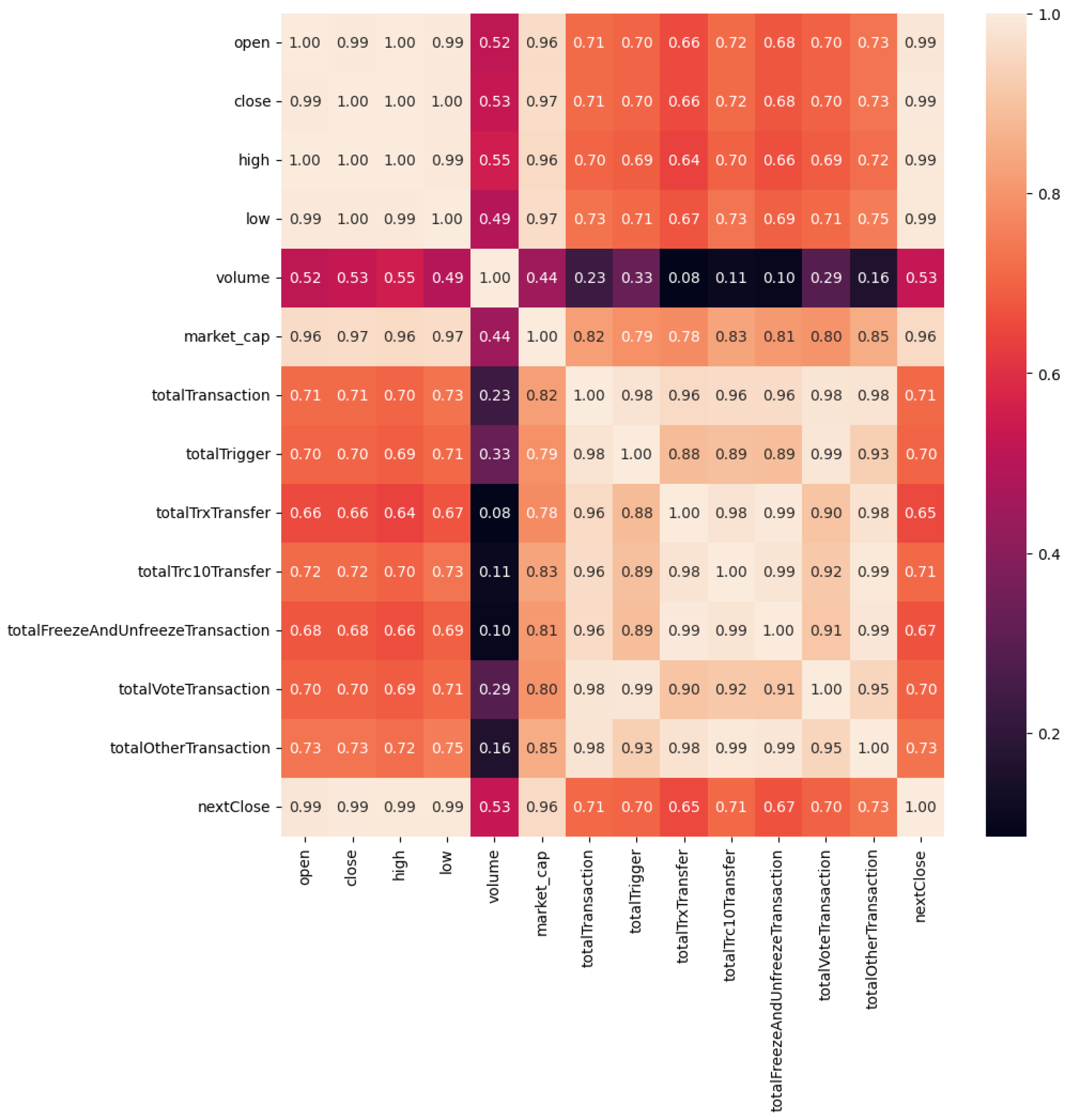The dataset is prepared from the data provided by Tronscan [46] website which manages the entire data of Tron cryptocurrency and ecosystem. We use the daily price which has high, low, and, day prices and the data containing the volumes of trades. We scale all our data to make the data of the same order (say between 1 to 10) using the standard scaler standardization technique. We use python to merge the uniform data for the same days for transaction success prediction. We chose the data carefully to obtain a better correlation and use relevant features that are useful in a market-based analysis. Features relevant to regression are concatenated, and a new dataset is created, merging the price dataset and the related dataset.

Figure 1 shows the heatmap showing the feature correlation. Some of the features show significant growth of the cryptocurrency and directly relate to strengthening the feature mentioned above and the scope of TRON. The daily price provides insights to the TRX coin market trends in short-term and prevailing market sentiments. The features such as ‘totalTrxTransfer’ and ‘totalTransactions’ refer to the transactions within the TRON environment, similar to the other features in Figure 1. In regression analysis, these features are useful in establishing correlation between different variables.

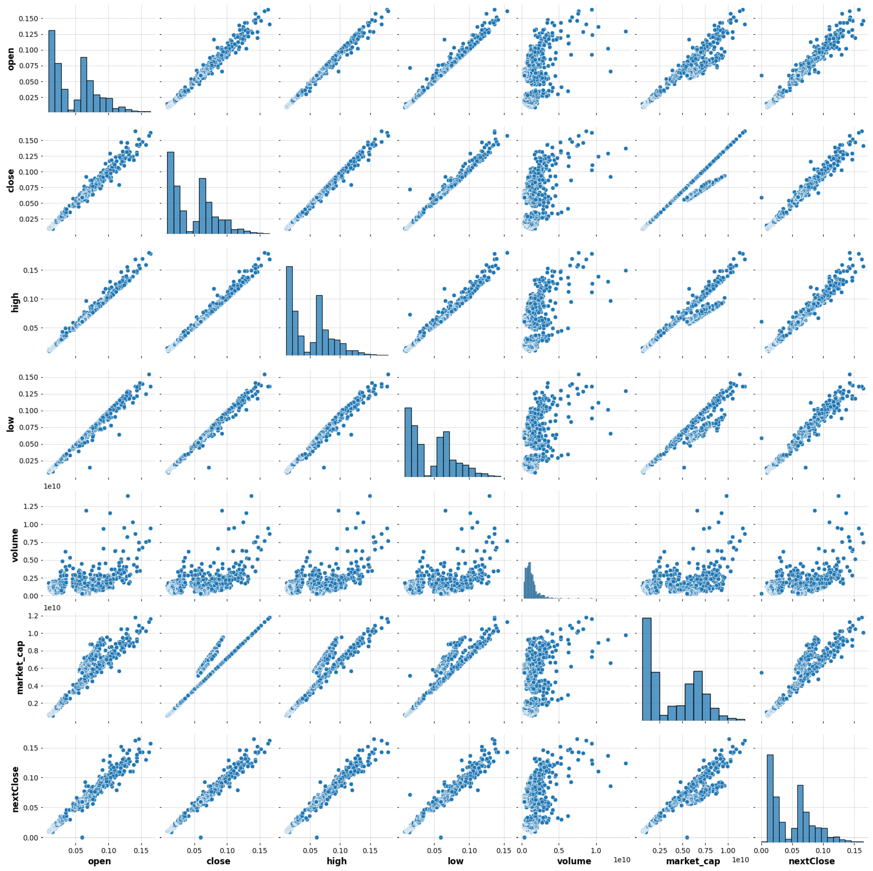
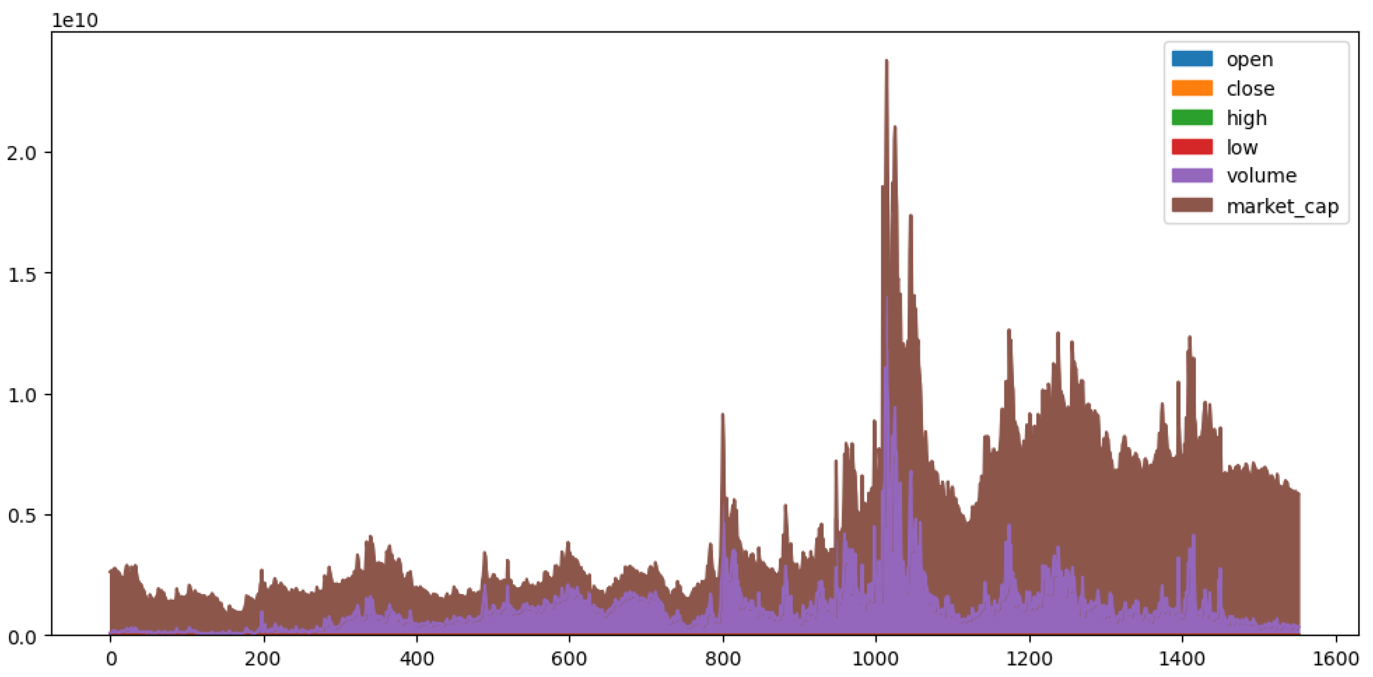
The relation between the values are plotted for the different features relating to the amount of Tron transferred from mid-2018 to mid-2022 and it is represented in Figure 2 and Figure 3. In Figure 2 the x-axis represents number of days and y-axis represents the numerical values of these features. This shows that market cap and volume have really high values compared to the rest of the features. Though there is a wealth of literature on cryptocurrency price prediction, only some methods are practical for use in real-time. Independent validation is therefore seen at a time of unexpected upheaval, but little difference in prices occurs during a period of bearish markets; this allows us to evaluate the accuracy of the predictions regardless of whether or not the market trend reverses between the two periods.

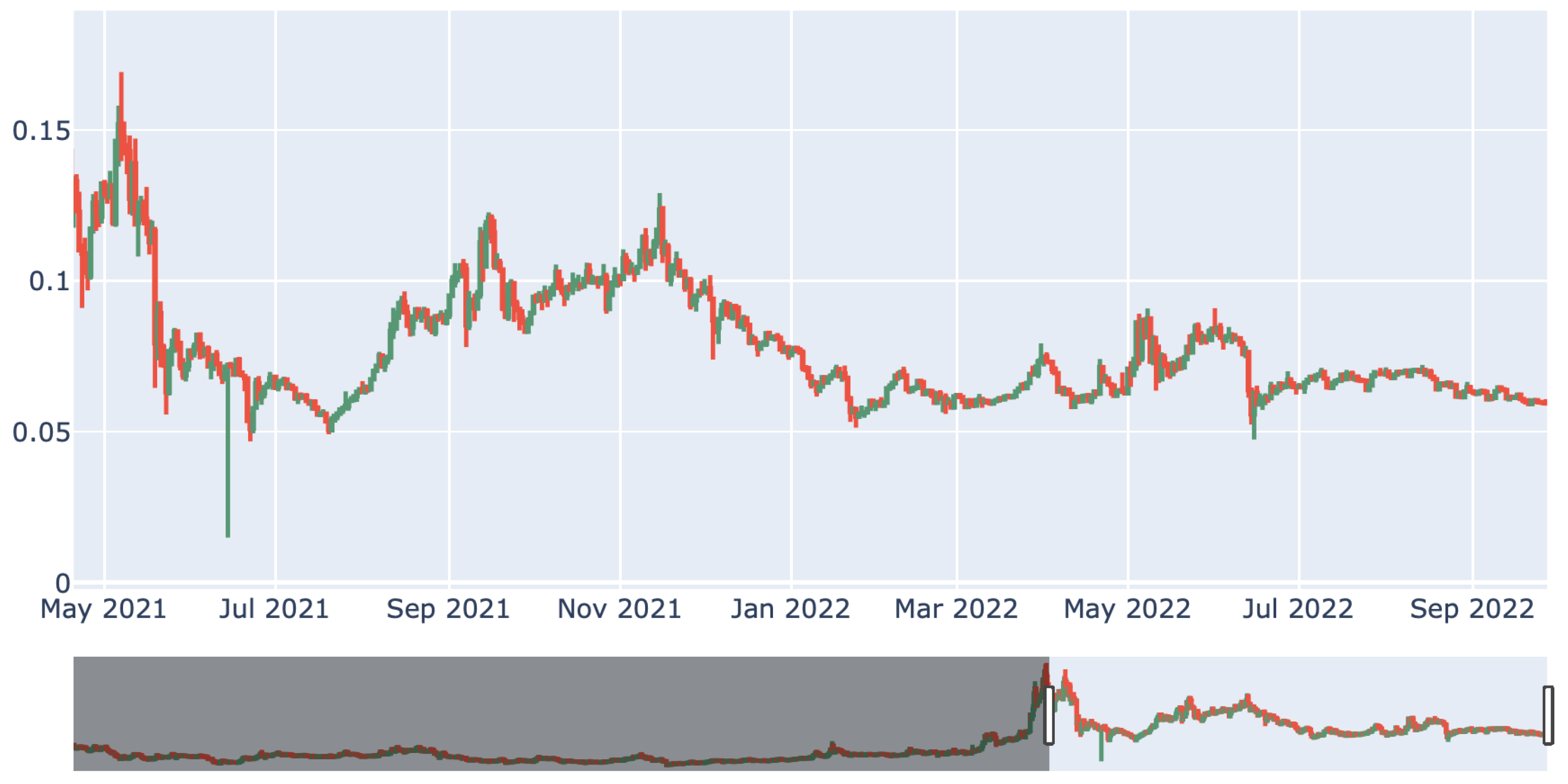
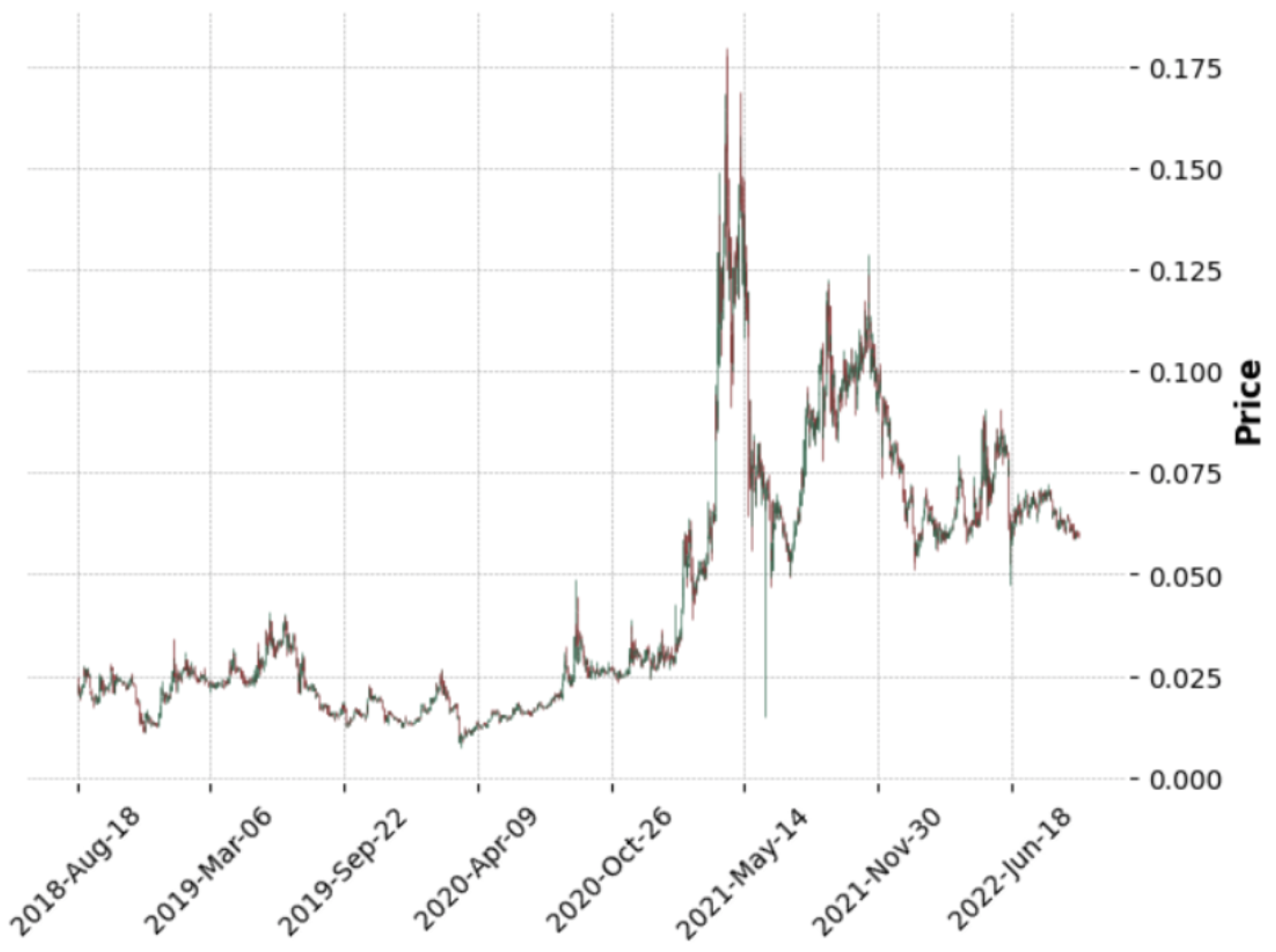
The use of cryptocurrencies as a novel medium for executing secure monetary transactions and storing value has grown in prominence in recent years. Due to the transparency of cryptocurrency transactions, quantitative analyses of many characteristics of virtual currencies are feasible. A candlestick chart condenses data from many time frames into a uniform price bar. They are, therefore, more beneficial than conventional open, high, low, and close (OHLC) bars or straight lines that connect closing price dots. The red candles represent fall in price and green candles represent the rise in prices. The candlestick chart for TRON is shown in Figure 4.

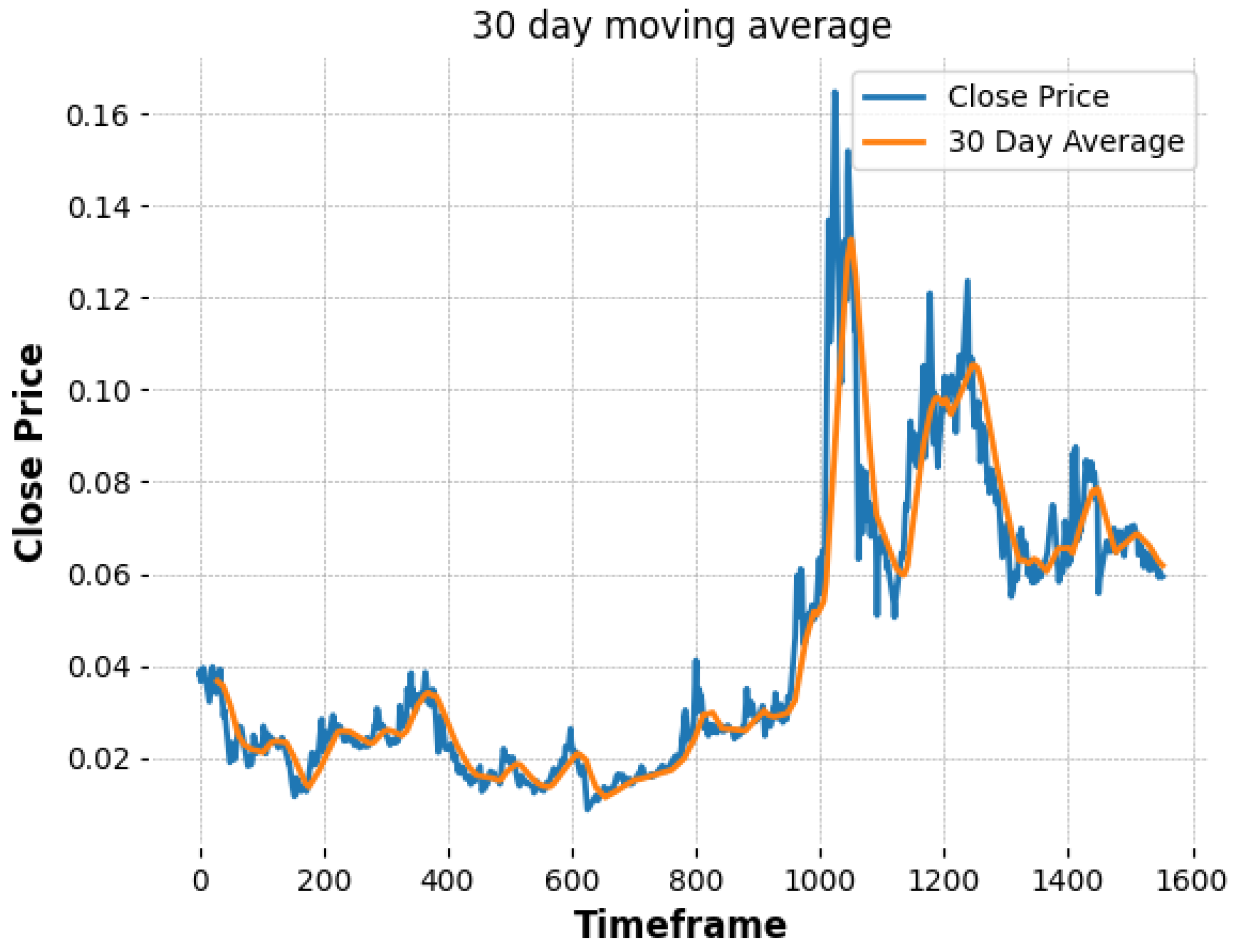
Figure 5 shows a 30-day moving average, which represents the closing price and the 30-day average price for four years. It is very clear from the plot that cryptocurrency, and in our case TRON has shown significant volatility over the 30 day average in the past, therefore we wish to help users make informed decisions for the long term but analysis would be beneficial to make these decisions (Figure 6 and Figure 7).

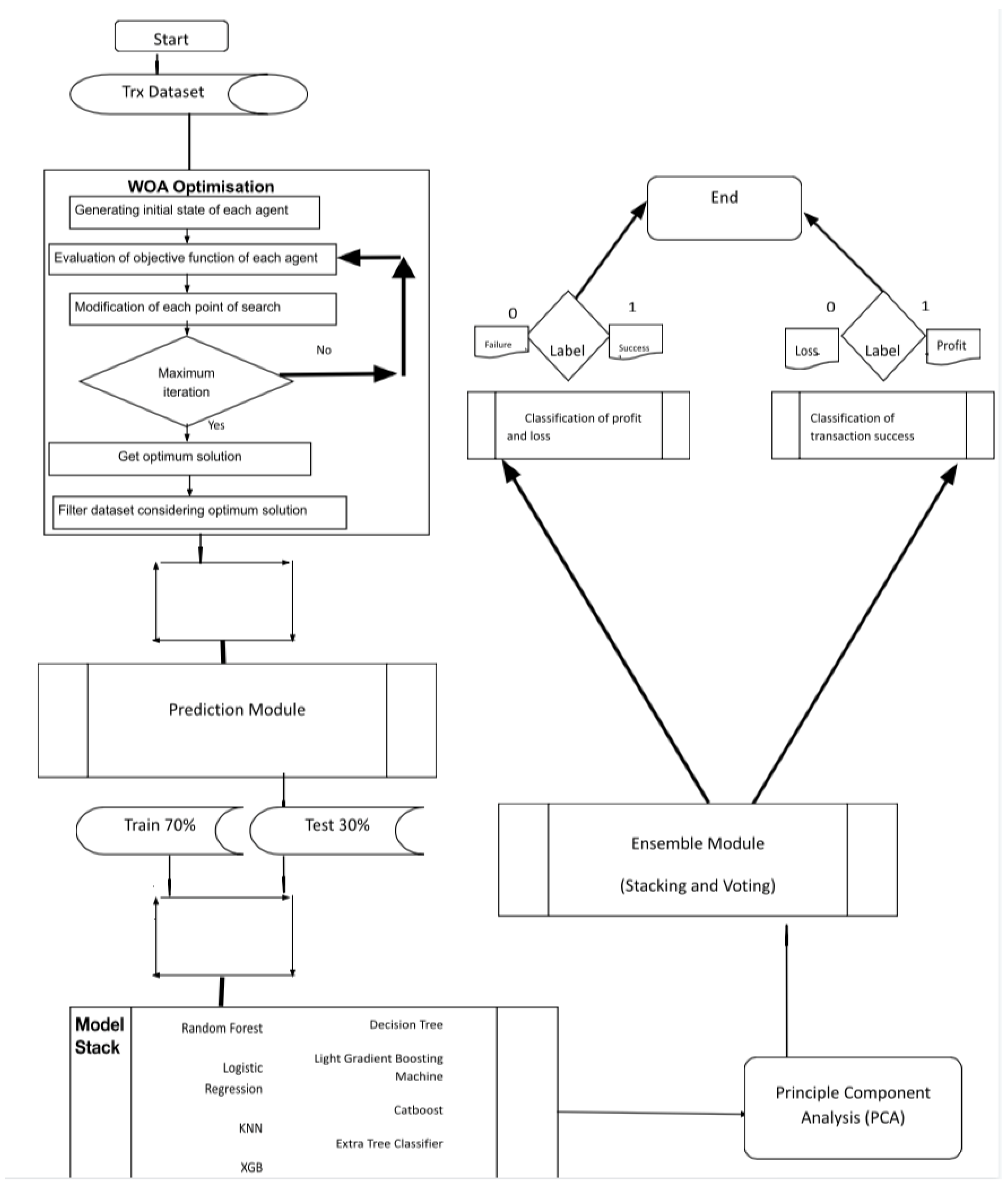
We propose an effective framework for potentially predicting future prices given the wide scope of TRON cryptocurrency and discuss aspects that have been neglected before. The aim a of studies such as this is to adapt to changing circumstances of the volatile nature of cryptocurrencies and the financial risks involved. The whale-optimized algorithm (WOA) is introduced along with ensemble classifiers, which can be called to train the models and more often results in improved accuracy and performance. The WOA algorithm is applied to obtain the optimized value and make a prediction on the transaction values. The Whale optimization algorithm is used for selecting the most optimal features for both of the predictions along with principal component analysis to potentially reduce the dimensionality of the data if applicable for the given scenario. The Returns (4) column indicates the percentage increase in the invested capital.

$$Returns\left[i\right]=Close\left[i\right]-Open\left[i\right]/Open\left[i\right]$$

(4)

A crucial parameter is the dayChange, which represents the fluctuations in the market on a day-to-day basis. Essentially, it is the difference between the closing prices of two consecutive days. Under certain circumstances, it may be given approximately by the modulus of difference of closing and opening prices. This is relevant for the closing price of the next day, calculating which is essential for price prediction.

$$dayChange\left[i\right]=Close\left[i\right]-Close[i-1]$$

(5)

OR

$$dayChange\left[i\right]=Close\left[i\right]-Open\left[i\right]$$

(6)

Changes in the daily prices can be expressed as shown in Equation (6). A binary variable CallOrder represents if trading on a specific day would result in a gain or loss, which can be derived by applying the unit step function to the DayChange.

$$callOrder\left[i\right]=Heaviside\left(dayChange\right[i\left]\right)$$

(7)

Likewise, the Equation (8) gives closing price of a cryptocurrency for a complex OHLC dataset.

$$Close\left[i\right]=f_{Simple}\left(Close[i-1]\right)$$

(8)

Now coming to the WOA optimization, we assume the actual best solution to be near the target fish (the solution) in an ocean and the other objects update their positions across the most optimal agent,

$$\overrightarrow{D}=\left|\overrightarrow{C}·{\overrightarrow{P}}_{\mathrm{best}}\left(t\right)-\overrightarrow{P}\left(t\right)\right|$$

(9)

In this context, “t” represents the current cycle, and the position vector of the humpback whale during its hunting strategy is denoted by $\overrightarrow{P}$. The best solution is represented by $X_{\ast }$, while coefficient vectors are denoted by $\overrightarrow{A}$ and $\overrightarrow{C}$. Essentially, $\overrightarrow{P}$ refers to the location of the humpback whale. This phase is often called encircling the fish. $\overrightarrow{a}$ represents the coefficient vector, which is used to control the exploration and exploitation rates of the algorithm, and $\overrightarrow{A}$ is the updated coefficient vector.

$$\overrightarrow{P}(t+1)={\overrightarrow{P}}_{\mathrm{best}}\left(t\right)-\overrightarrow{A}·\overrightarrow{D}$$

(10)

$$\overrightarrow{A}=2\overrightarrow{a}\ast \overrightarrow{k_1}-\overrightarrow{a}$$

(11)

Regarding the bubble-net attack stage, which is sometimes referred to as the exploitation stage, we utilize the process of shrinking to demonstrate how humpback whales surround their prey. As the iterations progress, the value of a certain variable, denoted as $\overrightarrow{C}$, is gradually reduced from 2 down to 0.

$$\overrightarrow{C}=2\overrightarrow{k_2}$$

(12)

Here, $\overrightarrow{k_1}$ and $\overrightarrow{k{2}_2}$ are random vectors in the range of [0, 1]. Variable m is used in the cosine function. Its value affects the direction and magniture of the steps taken towards the best solution. For the spiral updating position, the following functions are incorporated,

$${\overrightarrow{D}}^{\prime }=\left|{\overrightarrow{P}}_{\mathrm{best}}\left(t\right)-\overrightarrow{P}\left(t\right)\right|$$

(13)

$$\overrightarrow{P}(t+1)={\overrightarrow{D}}^{\prime }·cos\left(2\pi m\right)+{\overrightarrow{P}}_{best}\left(t\right)$$

(14)

In order for the humpbacks to update their position, the whales randomly search with respect to the position of their counterparts.

$$\overrightarrow{D}=\left|\overrightarrow{C}\ast {\overrightarrow{P}}_{rand}\left(t\right)-\overrightarrow{P}\left(t\right)\right|$$

(15)

$$\overrightarrow{P}(t+1)={\overrightarrow{P}}_{rand}\left(t\right)-\overrightarrow{A}·\overrightarrow{D}$$

(16)

Equation (17) calculates the coefficient $\mathbf{a}$ as iteration $\mathbf{t}$ progresses from 1 to $\mathbf{T}$.

$$a=2-t\times \frac{2}{T}$$

(17)

Equation (18) computes the center of the search space $\mathbf{C}$ by averaging positions of agents ${\mathbf{X}}_{\mathbf{i}}$.

$$C=\frac{1}{N}\sum _{i=1}^N{X}_i$$

(18)

Equation (19) calculates the distance $D_i$ between the current position $X_i$ of agent i and the best position A found so far, scaled by the coefficient a.

$$D_i=|C-a\times |A-X_i\left|\right|$$

(19)

Equation (20) computes the parameter $\mathbf{b}$ used for updating the position of agents based on the random values ${\mathbf{r}}_{\mathbf{1}}$ and ${\mathbf{r}}_{\mathbf{2}}$.

$$b=\frac{-1}{log(r_2\times \frac{A-X_i}{D_i})}$$

(20)

Equation (21) updates the position of agent i by moving it towards the best position A using a spiral-shaped movement when $r_1<0.5$.

$$X_i\leftarrow A-D_i\times e^{-b\times r_2}\times cos(2\times \pi \times r_2)$$

(21)

Equation (22) updates the position of agent $\mathbf{i}$ by moving it away from the best position A using a spiral-shaped movement when ${\mathbf{r}}_{\mathbf{1}}\ge \mathbf{0}.\mathbf{5}$.

$$X_i\leftarrow A+D_i\times e^{-b\times r_2}\times cos(2\times \pi \times r_2)$$

(22)

Equation (23) calculates the R-squared score ${\mathbf{r}}_{\mathbf{best}}$ as the final performance metric for the optimized regression model. ${\mathcal{D}}_{test}$ refers to the test data.

$$r_{best}\leftarrow r_{score}^2({\mathcal{D}}_{test}.target,\widehat{y})$$

(23)

Equation (24) calculates the distance between each agent and the best solution found so far.

$$D\leftarrow \mid C\times A-X\times a\mid$$

(24)

Equation (25) updates the position of each agent according to the Whale Optimization Algorithm.

$$X^{\prime }\leftarrow A-p\times D$$

(25)

Equation (26) predicts the class labels ${\displaystyle y_{pred}}$ for the test data ${\displaystyle x_{test}}$ using the optimized classifier ${\displaystyle clf}$.

$$y_{pred}=clf.predict\left(x_{test}\right)$$

(26)

The Equation (27) calculates the accuracy of the classifier by dividing the number of correct predictions by the total number of predictions made.

$$\mathrm{Accuracy}=\frac{\mathrm{Number}\mathrm{of}\mathrm{correct}\mathrm{predictions}}{\mathrm{Total}\mathrm{number}\mathrm{of}\mathrm{predictions}}$$

(27)

Equation (28) calculates the precision of the classifier, which is the proportion of true positive predictions out of all positive predictions made.

$$\mathrm{Precision}=\frac{\mathrm{True}\mathrm{Positives}}{\mathrm{True}\mathrm{Positives}+\mathrm{False}\mathrm{Positives}}$$

(28)

Equation (29) calculates the recall of the classifier, which is the proportion of true positive predictions out of all actual positive instances in the dataset.

$$\mathrm{Recall}=\frac{\mathrm{True}\mathrm{Positives}}{\mathrm{True}\mathrm{Positives}+\mathrm{False}\mathrm{Negatives}}$$

(29)

Equation (30) computes the F1 score, which is the harmonic mean of precision and recall. The F1 score is a popular metric used to evaluate classifiers when dealing with imbalanced datasets.

$$\mathrm{F}1\_\mathrm{Score}=2·\frac{\mathrm{Precision}·\mathrm{Recall}}{\mathrm{Precision}+\mathrm{Recall}}$$

(30)

In Equation (31) C is the confusion matrix, $y_{test}$ are the true class labels, and $y_{pred}$ are the predicted class labels. The confusion matrix C is a square matrix of size $k\times k$, where k is the number of classes. Each element $C_{ij}$ represents the number of instances of class i that were classified as class j.

$$C=\mathrm{confusion}\_\mathrm{matrix}(y_{test},y_{pred})$$

(31)

In Algorithm 1, first, the population of profit classifications, denoted as $\mathbf{P}\_\mathbf{i}$, is initialized. The training sets are split into n folds using Repeated Stratified K-fold cross-validation. The first n-1 folds are used as the base model, and the predictions are made for the n-th fold. The predictions from steps 1, 2, and 3 are concatenated into the x1_train list. The list is the converted to its binary representation and the fitness of each solution in the population is computed followed by initialisation of best solution as ${\mathbf{P}}^{\ast }$. After processing each solution, the algorithm checks if any search agent has moved beyond the search space and corrects the position if necessary. The list is again converted to its binary representation and the fitness of each search agent is computed. The iteration counter t is incremented. Finally, the algorithm returns the best solution ${\mathbf{P}}^{\ast }$. All the relevant equations are explained in Equations (9)–(16) related to this algorithm. This is the general algorithm for implementation of Whale optimization algorithm and is applicable for similar cryptocurrency datasets (or a retrieved OHLC data). It is worth noting that using A = 1 can lead to slower convergence to the global optimum, as it does not allow for larger jumps in the search space. It may be beneficial to use larger values of A to allow for more exploration of the search space. At each iteration of the algorithm, a new set of candidate parameter values is generated using a combination of random mutation and cross-over (i.e., taking the best parts of two or more candidate solutions and combining them). These new solutions are then evaluated using the objective function, and the best ones are kept as the basis for the next iteration. This gives us the best value of the hyper-parameters to then train our model. The algorithm converges on a set of parameter values that produce a high-performing classification model, as measured by the objective function. The algorithm may need to be run several times with different starting parameters in order to find the best possible solution. A good number of iterations is 100 in general, though the algorithm in itself is very complex, and more almost always lead to having a higher probability of finding a better solution.

Algorithm 1 Optimal Global Position Vector

1: procedure OptimalGlobalPosition($I,P$)   2:    Initialize the population $P_i$$(i=1,2,3,\dots ,N)$ of profit classification.   3:    Split the training sets into n folds using Repeated Stratified K-fold.   4:    Take the first fold of the base model as $n-1$, n-th folds are to be predicted.   5:    The predictions using steps 1, 2, and 3 are concatenated to the $x1\_train$ list.   6:    Convert the list to binary representation.   7:    Compute the fitness of each solution.   8:    Set the best solution as $P^{\ast }$.   9:    while $(t<I)$ do 10:     for each solution do 11:      if $(p<\frac{1}{2})$ then 12:        if $\left(\right|A|<1)$ then 13:          The particle position is updated by $\overrightarrow{D}=\left|\overrightarrow{C}\odot {\overrightarrow{P}}_{\mathrm{rand}}\left(t\right)-\overrightarrow{P}\left(t\right)\right|$ 14:        else 15:          if $\left(\right|A|>1)$ then 16:          Select a random particle $P_{\mathrm{rand}}$. 17:          Update the particle position by $\overrightarrow{P}(t+1)={\overrightarrow{P}}_{\mathrm{rand}}\left(t\right)-\overrightarrow{A}\odot \overrightarrow{D}$. 18:          end if 19:        end if 20:      end if 21:     end for 22:     Investigate whether any search agent moves beyond space and correct the sample. 23:     Convert the list to binary representation. 24:     Compute the fitness of every search agent. 25:     Update $P^{\ast }$ if there is a better solution. 26:     $t=t+1$. 27:    end while 28:    return $P^{\ast }$. 29: end procedure

Algorithm 2, titled “Whale Optimization Algorithm for Regression”, aims to optimize the regression models (e.g., LightGBM, XGBoost, CatBoost) for achieving the best R-squared score using the Whale Optimization Algorithm. The algorithm takes as input the training data $\mathcal{D}\mathbf{train}$, testing data $\mathcal{D}\mathbf{test}$, a set of regression models $\mathbf{M}$, a search space $\mathbf{S}$, the number of agents $\mathbf{N}$, and the number of iterations $\mathbf{T}$. The main objective of the algorithm is to find the best combination of hyperparameters for the chosen regression model.

The FitnessFunction is defined to measure the performance of a solution by fitting the model to the training data and predicting the target variable on the test data. The fitness function returns the negative R-squared score to guide the optimization process. All the equations related to Algorithm 2 are explained in Equations (17)–(23) and (32)–(34).

Algorithm 2 Whale Optimization Algorithm for Regression

Require:  Training data ${\mathcal{D}}_{train}$, testing data ${\mathcal{D}}_{test}$, regression models M (e.g., LightGBM, XGBoost, CatBoost), search space S, number of agents N, number of iterations T Ensure:  Best R-squared score $r_{best}$ found   1: function FitnessFunction($X,M,{\mathcal{D}}_{train},{\mathcal{D}}_{test}$)   2:    $x_{train}\leftarrow$ DataFrame(X, columns = ${\mathcal{D}}_{train}$.columns)   3:    M.fit($x_{train}$, ${\mathcal{D}}_{train}$.target)   4:    $\widehat{y}\leftarrow M$.predict(${\mathcal{D}}_{test}$)   5:    return $-r_{score}^2({\mathcal{D}}_{test}$.target, $\widehat{y})$   6: end function   7: $X\leftarrow$ RandomUniform($low=S_{low},high=S_{high},size=(N,S_{dim})$)   8: $A\leftarrow$ None   9: $r_{best}\leftarrow -\infty$ 10: for $t=1$ to T do 11:    $a\leftarrow 2-t\times \frac{2}{T}$ 12:    $C\leftarrow \frac{1}{N}{\sum }_{i=1}^N{X}_i$ 13:    for $i=1$ to N do 14:     Clip $X_i$ to S 15:     $f_i\leftarrow$FitnessFunction($X_i,M,{\mathcal{D}}_{train},{\mathcal{D}}_{test}$) 16:     if $f_i>r_{best}$ then 17:      $r_{best}\leftarrow f_i$ 18:      $A\leftarrow X_i$ 19:     end if 20:     $D_i\leftarrow |C-a\times |A-X_i\left|\right|$ 21:     $r_1,r_2\leftarrow$ RandomUniform(0, 1) 22:     $b\leftarrow \frac{-1}{log(r_2\times \frac{A-X_i}{D_i})}$ 23:     if $r_1<0.5$ then 24:      $X_i\leftarrow A-D_i\times e^{-b\times r_2}\times cos(2\times \pi \times r_2)$ 25:     else 26:      $X_i\leftarrow A+D_i\times e^{-b\times r_2}\times cos(2\times \pi \times r_2)$ 27:     end if 28:    end for 29: end for 30: $x_{train\_best}\leftarrow$ DataFrame(A, columns = ${\mathcal{D}}_{train}$.columns) 31: M.fit($x_{train\_best}$, ${\mathcal{D}}_{train}$.target) 32: $\widehat{y}\leftarrow M$.predict(${\mathcal{D}}_{test}$) 33: $r_{best}\leftarrow r_{score}^2({\mathcal{D}}_{test}$.target, $\widehat{y})$ 34: return $rbest$

The algorithm initializes the positions of $\mathbf{N}$ agents in the search space and iterates for a given number of iterations $\mathbf{T}$. In each iteration, the algorithm updates the agents’ positions according to the Whale Optimization Algorithm equations, which involve calculating the distance between each agent and the best solution found so far. The agents’ positions are updated based on random variables and the distances calculated. The agents’ positions are clipped to the search space to ensure they remain within the search space boundaries. The fitness of each agent is evaluated, and the best solution is updated if a better one is found. The R-squared score is calculated for the best solution at the end of the algorithm, and the best R-squared score is returned.

The Algorithm 3 uses various variables, including $\mathcal{D}\mathbf{train}$ and $\mathcal{D}\mathbf{test}$, which represent the training and testing data, respectively. The variable $\mathbf{M}$ represents a set of classification models, such as Logistic Regression and Random Forest. The search space for the optimization process is denoted by $\mathbf{S}$, while the number of agents in the search space is represented by $\mathbf{N}$. The algorithm runs for a specified number of iterations, indicated by T. The positions of agents within the search space are stored in $\mathbf{X}$. The position of the best solution found so far is represented by $\mathbf{A}$, and the best accuracy score achieved is denoted by ${\mathbf{a}}_{\mathbf{best}}$. The equations used in Algorithm 3 are explained in Equations (17), (18), (24), (25) and (32)–(34). ${\mathbf{S}}_{\mathbf{dim}}$ refers to the dimensions of the desired output shape for the array generated by the ‘RandomUniform’ function, containing uniformly distributed numbers between 0 and 1. The notation “:-1” is a slicing notation which means “all elements from the start to one before the end”.

Algorithm 3 Whale Optimization Algorithm for Classification using Stacking and Voting Classifiers

Require:  Training data $\mathcal{D}train$, testing data $\mathcal{D}test$, classification models M (e.g., Logistic Regression, Random Forest, K-Nearest Neighbors, Gaussian Naive Bayes, Stochastic Gradient Descent, Decision Tree, Extra Trees), search space S, number of agents N, number of iterations T Ensure:  Best accuracy score $a_{best}$ found for the classifiers   1: function FitnessFunction($X,M,\mathcal{D}train,\mathcal{D}test$)   2:    $x_{train}\leftarrow$ DataFrame($\mathcal{D}train$.iloc[:, :-1], columns = $\mathcal{D}train$.columns[:-1])   3:    $x_{test}\leftarrow$ DataFrame($\mathcal{D}test$.iloc[:, :-1], columns = $\mathcal{D}test$.columns[:-1])   4:    $y_{train}\leftarrow$$\mathcal{D}train$.target   5:    $estimators\leftarrow$ []   6:    for $m\in M$ do   7:     $pipe\leftarrow$ Pipeline([(m, $m\left(\right)$)])   8:     $estimators$.append((m$.class.name$, $pipe$))   9:    end for 10:    $voting\leftarrow$ VotingClassifier(estimators = estimators, voting = ‘soft’) 11:    $stacking\leftarrow$ StackingClassifier(estimators = estimators, final_estimator = voting) 12:    $stacking.fit(xtrain,y_{train})$ 13:    $score\leftarrow$ stacking.score($x_{test}$, $\mathcal{D}test$.target) 14:    return $score$ 15: end function 16: $X\leftarrow$ RandomUniform($low=Slow,high=S_{high},size=(N,S_{dim})$) 17: $A\leftarrow$ None 18: $a_{best}\leftarrow 0$ 19: for $t=1$ to T do 20:    $a\leftarrow 2-t\times \frac{2}{T}$ 21:    $C\leftarrow \frac{1}{N}{\sum }_{i=1}^N{X}_i$ 22:    for $i=1$ to N do 23:     Clip $X_i$ to S 24:     $f_i\leftarrow$FitnessFunction($X_i,M,\mathcal{D}train,\mathcal{D}test$) 25:     if $f_i>a_{best}$ then 26:      $A\leftarrow X_i$ 27:      $a_{best}\leftarrow f_i$ 28:     end if 29:    end for 30:    $p\leftarrow$ RandomUniform($size=S_{dim}$) 31:    $D\leftarrow \mid C\times A-X\times a\mid$ 32:    $X^{\prime }\leftarrow A-p\times D$ 33: end for 34: $x_{trai{n}_{b}est}\leftarrow$ DataFrame(A, columns = $\mathcal{D}train$.columns[:-1]) 35: $stacking$.fit($x_{trai{n}_{b}est}$, $\mathcal{D}train$.target) 36: $abest\leftarrow stacking.score(x_{test},\mathcal{D}test$.target) 37: return $abest$

The methodology of applying the algorithm consists of three steps:

• Applying the Regression Techniques; Gradient boosting regressors have been very successful in price prediction-based regression. XGBoost, CATBoost, and LGBM regressors are used for dynamic pricing estimation and we compare the efficiency of these regressors for our prepared TRX dataset. The tree-based regressors such as XGBoost, CatBoost, and LightGBM are useful in regressors have feature selection capabilities built-in that help identify the most important features for the regression task. The libraries are useful regularization techniques to prevent overfitting. XGBoost, CatBoost, and LightGBM can still be significantly faster than other algorithms when used along with a meta-heuristic.
• Classification using standard classifiers; After the regression, we move on to the classification of profit and loss using different classifiers. We divide the data into training and testing sets and the training data are used to train each model simultaneously.
• Classification using an ensemble of classifiers; The next stage is to analyze the forecasts of the models. Accuracy may be improved by ensemble techniques with XGBoost when dealing with asymmetric data. We first focus on classifying profits and losses to check if there is a profit, followed by an inspection of the accuracy of transaction success & failure considering TRX transactions over Blockchain. Equations (27)–(31) give more explanation about the evaluation metrics used.

XGBoost, CATBoost, and LGBM regressors are used for the regression.

Table 1. Analysis of Regression algorithms with R squared, RSME, MAE and EV as metrics.

Regressor Model	R Squared	RMSE	MAE	Explained Variance
XGBoost Regressor	0.982032	0.004142	0.002027	0.982040
CATBoost Regressor	0.985809	0.003775	0.002028	0.984824
LGBM Regressor	0.982514	0.004003	0.001916	0.982536

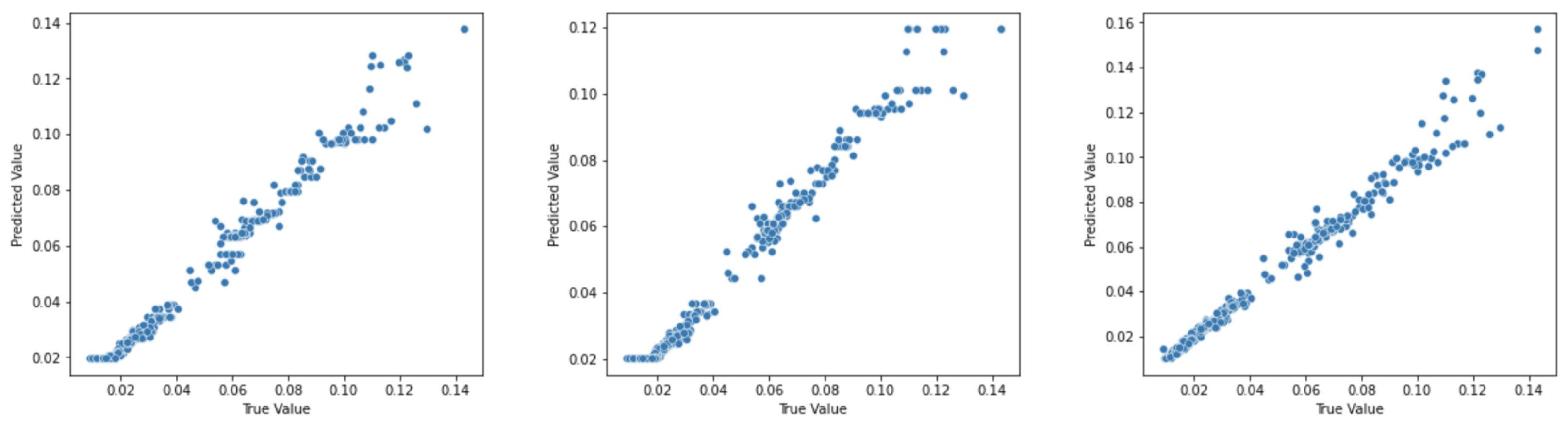
shows the different metrics for regressions performed by the models. Figure 8 shows the scatter plots for corresponsing (a). XGBoost regressor, (b). LGBM regressor and (c). CATBoost Regressor. A higher R2 score generally indicates that the model is a better fit to the data. It is given by $R^2=1-(SSres/SStot)$ where SSres is the squared residuals (the difference between the predicted and actual values) and SStot is the total sum of squares (i.e., the differences between the actual values and the mean of the target variable).

4. Results and Discussion

The x-axis of each scatterplot shows the true values of the next day’s closing price, while the y-axis shows the predicted values of the next day’s closing price. The scatterplots are useful for visualizing how well the models perform in predicting the next day’s closing price of Tron. The closer the scatterplot points are to the line of perfect predictions (y = x), the better the model is at predicting the next day’s closing price of Tron.

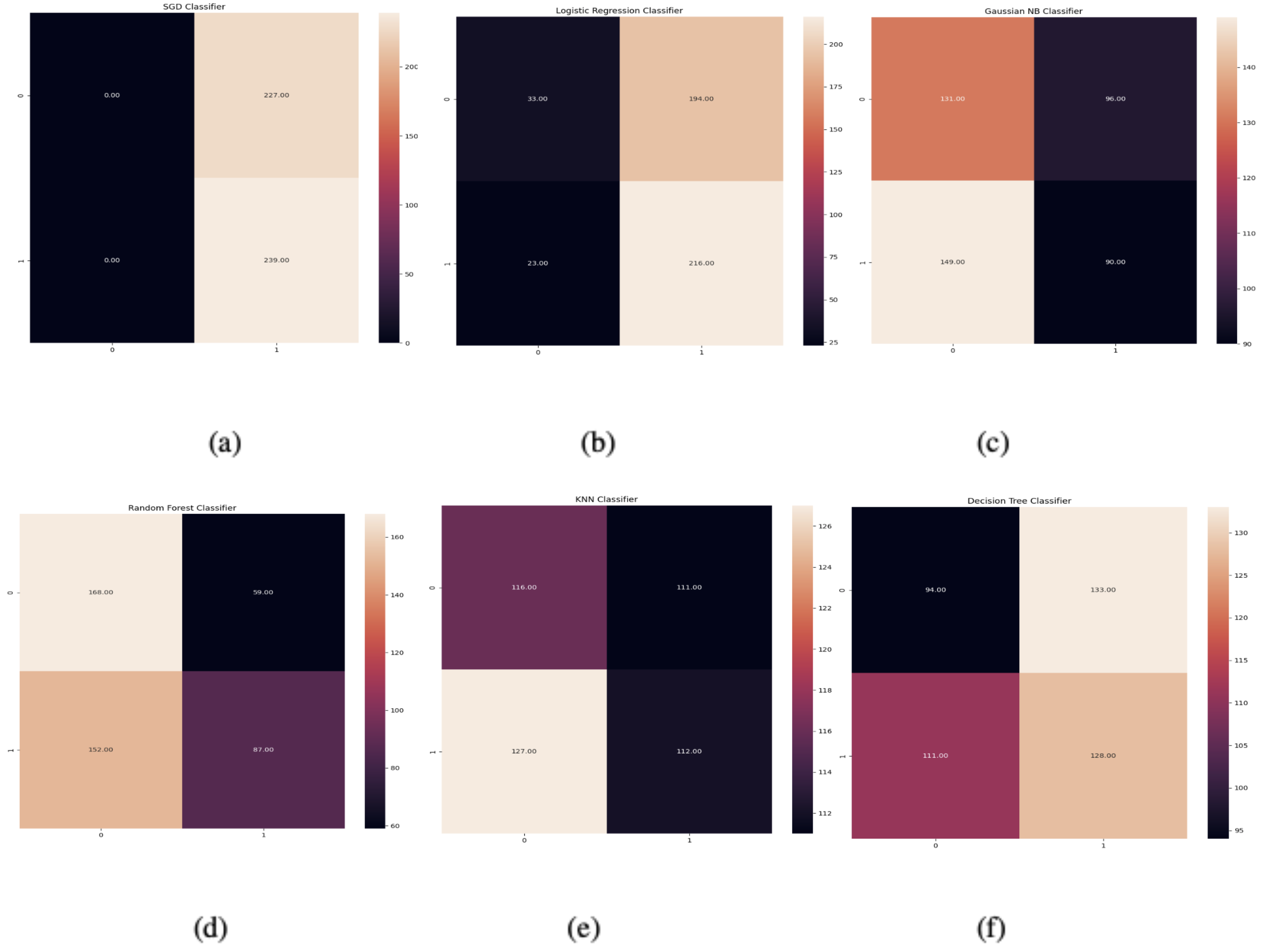
We then move to the classification problem, which helps with determining whether the cryptocurrency is going to make a profit or loss the next day based on the historical performance of the TRX coin. It is essential to consider that the price of any cryptocurrency, as noted in the literature review, can fluctuate significantly depending on factors that impact the market and factors inherent to the nature of the blockchain technology. For our classification problems, we analysed the performance of several models and observed that tree based models perform the best when it comes to smaller datasets. It is reflected in our analytics by the XGBoost classifier, which uses a tree-based gradient boosting algorithm. It is important to reduce its complexity to minimize any overfitting, which is effectively performed using L2 regularization and manual tuning while not including these hyper-parameters when defining the search space. The voting classifier takes several tree-based classifiers as inputs along with the other models, similar to stacking the classifier but in a more effective way.

We found that the accuracy of the models such as Random Forest, Decision Tree, Gaussian Naive Baise, Logistic Regression, K-Nearest Neighbors, Scholastic Gradient Descent is on the lower end when compared to these ensemble techniques. The stacking classifier uses all these models plus the gradient boosters as pipelines with the final estimator being the voting classifier. Hyperparameter optimization then sets the ideal settings for learning rate, booster type, maximum depth, number of estimators, and other factors classifiers in our tabular dataset. From the standard techniques, XGBoost provides the best accuracy because of its superior performance in tabular datasets and tree-based structures. The corresponding confusion matrix before applying WOA is shown in Figure 9. The use of a meta-heuristic whale optimization algorithm with staking classifier tends to bypass local optima.

In Algorithm 1, Equation (32) initializes the positions of the agents in the search space $\mathbf{X}$ with random values uniformly distributed between the lower and upper limits of the search space $({\mathbf{S}}_{\mathbf{low}}$ and ${\mathbf{S}}_{\mathbf{high}})$, and with a size of $(\mathbf{N},{\mathbf{S}}_{\mathbf{dim}})$.

$$X\leftarrow RandomUniform(low=S_{low},high=S_{high},size=(N,S_{dim})$$

(32)

Similarly, Equation (33) gives random numbers in the range [0, 1] used for updating the positions of agents.

$$r_1,r_2\leftarrow RandomUniform(0,1)$$

(33)

Equation (34) creates a new DataFrame named ${\mathbf{x}}_{\mathbf{train}\_\mathbf{best}}$ using the best agent’s position $\mathbf{A}$. The DataFrame is created with the same column names as the training data ${\mathcal{D}}_{\mathbf{train}}$. This is performed to ensure that the data structure is consistent with the input format required by the regression models.

$$x_{train\_best}\leftarrow pd.DataFrame(A,columns={\mathcal{D}}_{train}.columns)$$

(34)

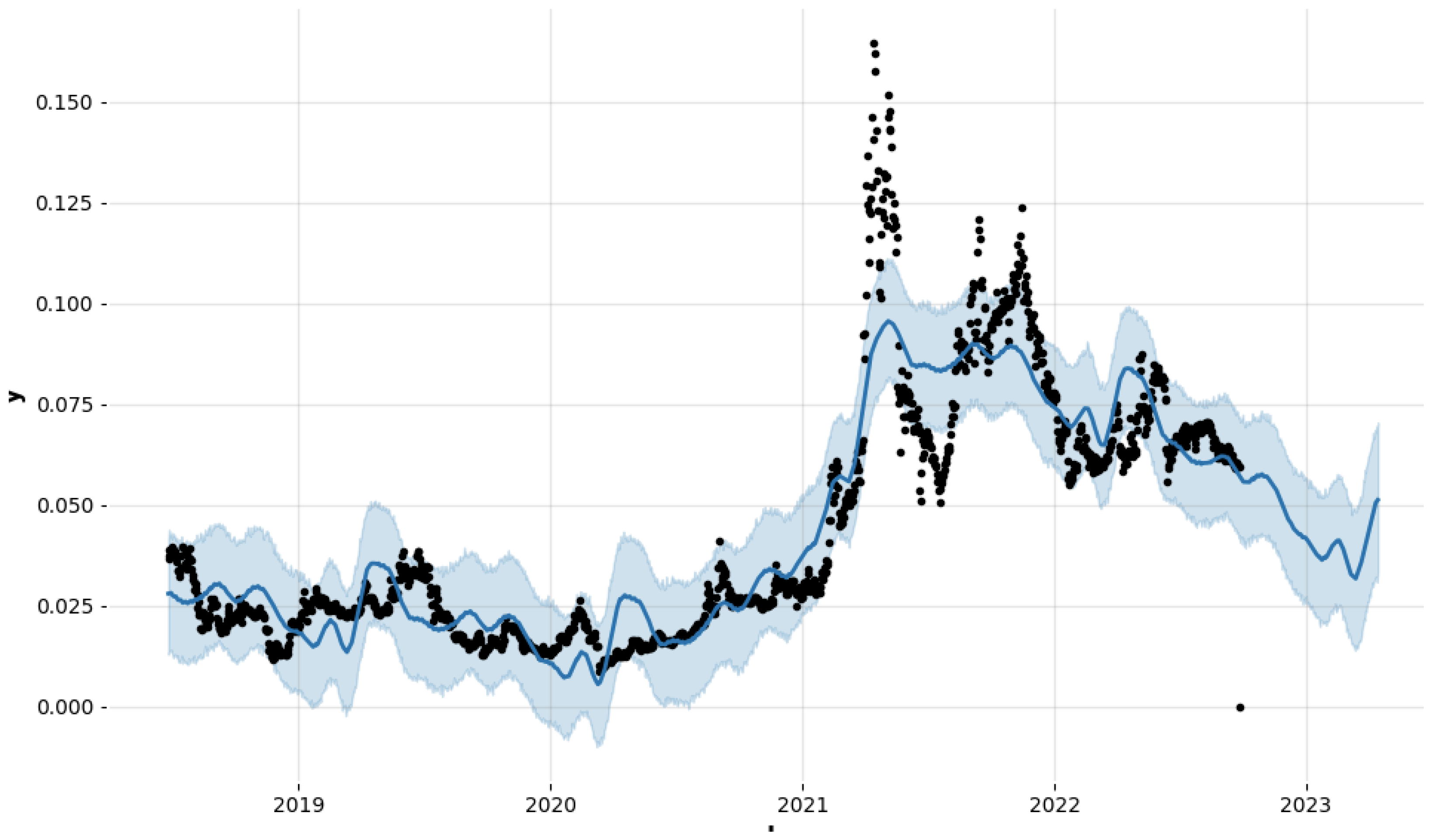
Comparing the models, CatBoost seems to perform slightly better than the other two models, with the highest R-squared value, lowest MSE and RMSE, and a slightly higher median absolute error (MedAE) than LGBM. However, the differences in performance are relatively small, and all of the models perform quite well. Techniques such as regularization or early stopping are useful and help prevent overfitting to a certain extent. The optimization algorithm does a good job in training the model in a more efficient and effective manner, which could indirectly help in reducing overfitting. However, reducing the complexity of the model by not considering the parameters which lead to a more complex model is a good approach to tackle the problem of overfitting along with regularization and cross-validation. Although the SGD classifier gets no true positive or false negative. This situation often arises when the model predicts only one class for all instances. The WOA addressed this by correct hyperparameters, with the results as shown in graphs and tables. Now, the prophet forecaster shows the prediction for future dates based on the current dates in the dataset. It is depicted in Figure 10.

Table 2. Most important Hyper parameters considered for the training purpose, only relevant hyper parameters are searched using WOA.

Regressor Model	Hyper Parameters Used
XGBoost Regressor	subsample, eta, booster, min_child_weight, learning_rate colsample_bytree, validate_parameters, and nthread
CATBoost Regressor	subsample, random_strength, learning_rate, l2_leaf_reg, colsample_bylevel, bagging_temperature, and boosting_type
LGBM Regressor	subsample, learning_rate, colsample_bytree, max_bin, objective, min_data_in_leaf, and feature_fraction

shows some of the hyper-parameters that are included in the search to be tuned during the training of these models. It is important to note that n_estimators, reg_alpha or reg_lambda, min_data_in_leaf, min_gain_to_split should be preferred to be manually tuned to avoid overfitting, and any other hyperparameter should be accessed for overfitting on a case by case basis. Cross-validation (5, 8 or 10 folds) must be performed for accessing if there is overfitting and lower performance on testing data with respect to the corresponding training data.

We then move to the classification problem, which helps with determining whether the cryptocurrency is going to make a profit or loss the next day based on the historical performance of the TRX coin. It is essential to consider that the price of any cryptocurrency, as noted in the literature review, can fluctuate significantly depending on factors that impact the market and factors inherent to the nature of the blockchain technology.

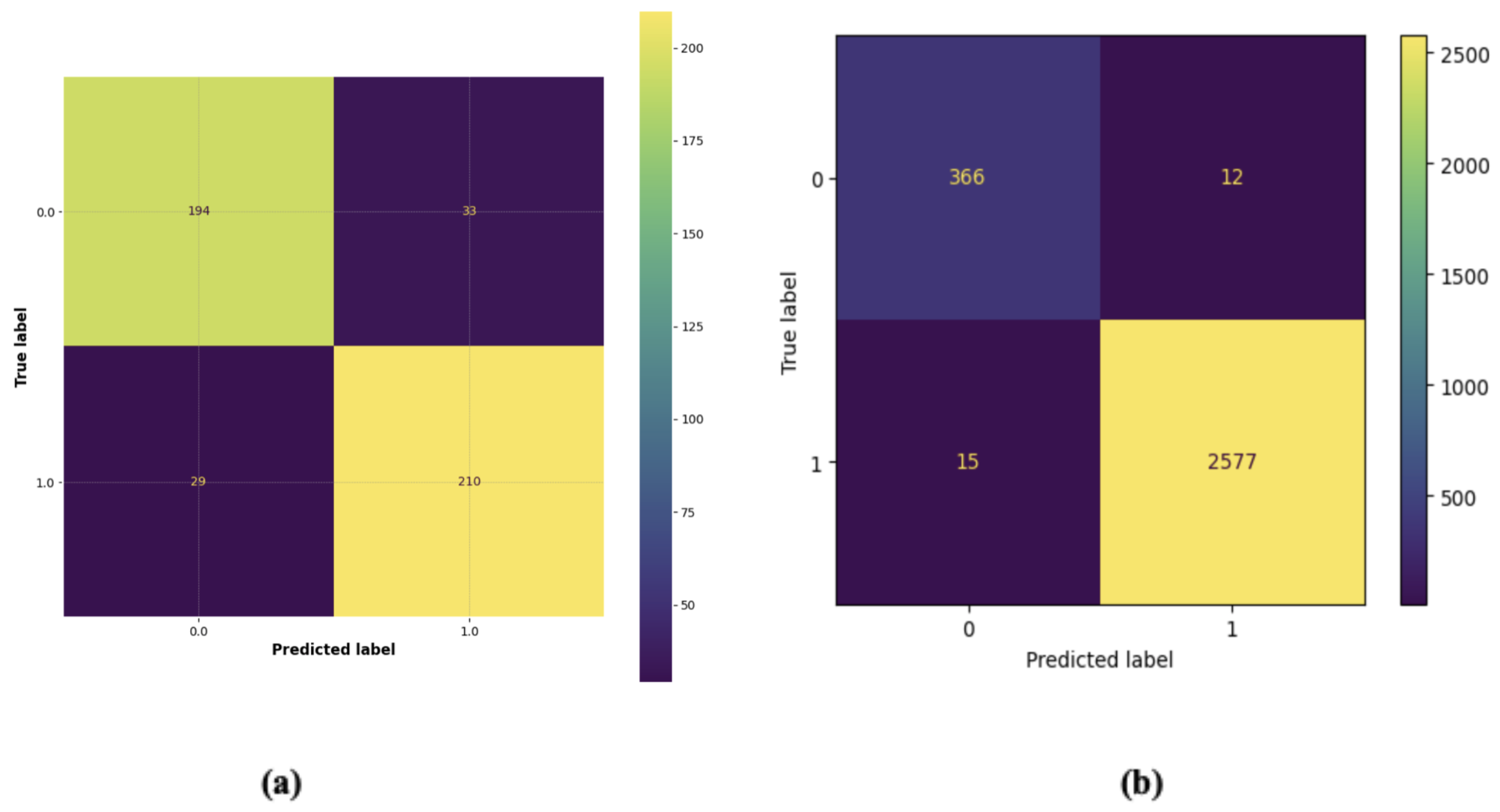
For our classification problems, we analysed the performance of several models and observed that tree based models perform the best when it comes to smaller datasets. It is reflected in our analytics by the XGBoost classifier, which uses a tree-based gradient boosting algorithm. It is important to reduce its complexity to minimize any overfitting, which is effectively performed using L2 regularization and manual tuning while not including these hyper-parameters when defining the search space. The voting classifier takes several tree-based classifiers as inputs along with the other models, similar to stacking the classifier but in a more effective way. We found that the accuracy of the models such as Random Forest, Decision Tree, Gaussian Naive Baise, Logistic Regression, K-Nearest Neighbors, Scholastic Gradient Descent is on the lower end when compared to these ensemble techniques. The stacking classifier uses all these models plus the gradient boosters as pipelines with the final estimator being the voting classifier. Hyperparameter optimization then sets the ideal settings for learning rate, booster type, maximum depth, number of estimators, and other factors classifiers in our tabular dataset. From the standard techniques, XGBoost provides the best accuracy because of its superior performance in tabular datasets and tree-based structures. The corresponding confusion matrix of the model is shown in Figure 11. The use of a meta-heuristic whale optimization algorithm with staking classifier tends to bypass local optima.

This is evident from the results that the base model has distinct performance over the dataset for the next day prediction. The dataset is relatively small, so the accuracy of these base models is found to be quite close to each other. The dataset for price prediction is quite balanced; however, the test set does not have many values to make accurate predictions. This is not much of a problem since tree-based models perform well even on this small dataset and perform exceedingly well when used in stacking and voting modules. The training and testing are first carried out using different machine learning classifiers with a test-train split of 30–70; next, we use it with the proposed stacking and the voting-based ensemble models. Random Forest, Support Vector Classifier, Decision Tree Classifier, ExtraTrees Classifier, Light Gradient Boosting Classifier, XGBoost, and Logistic Regression Classifier are some of the classifiers used by the stacking model. Each of these models provided appreciable accuracy when used alone, but the number of false negatives and false positives varied greatly. This is subsequently reflected in the recall graph.

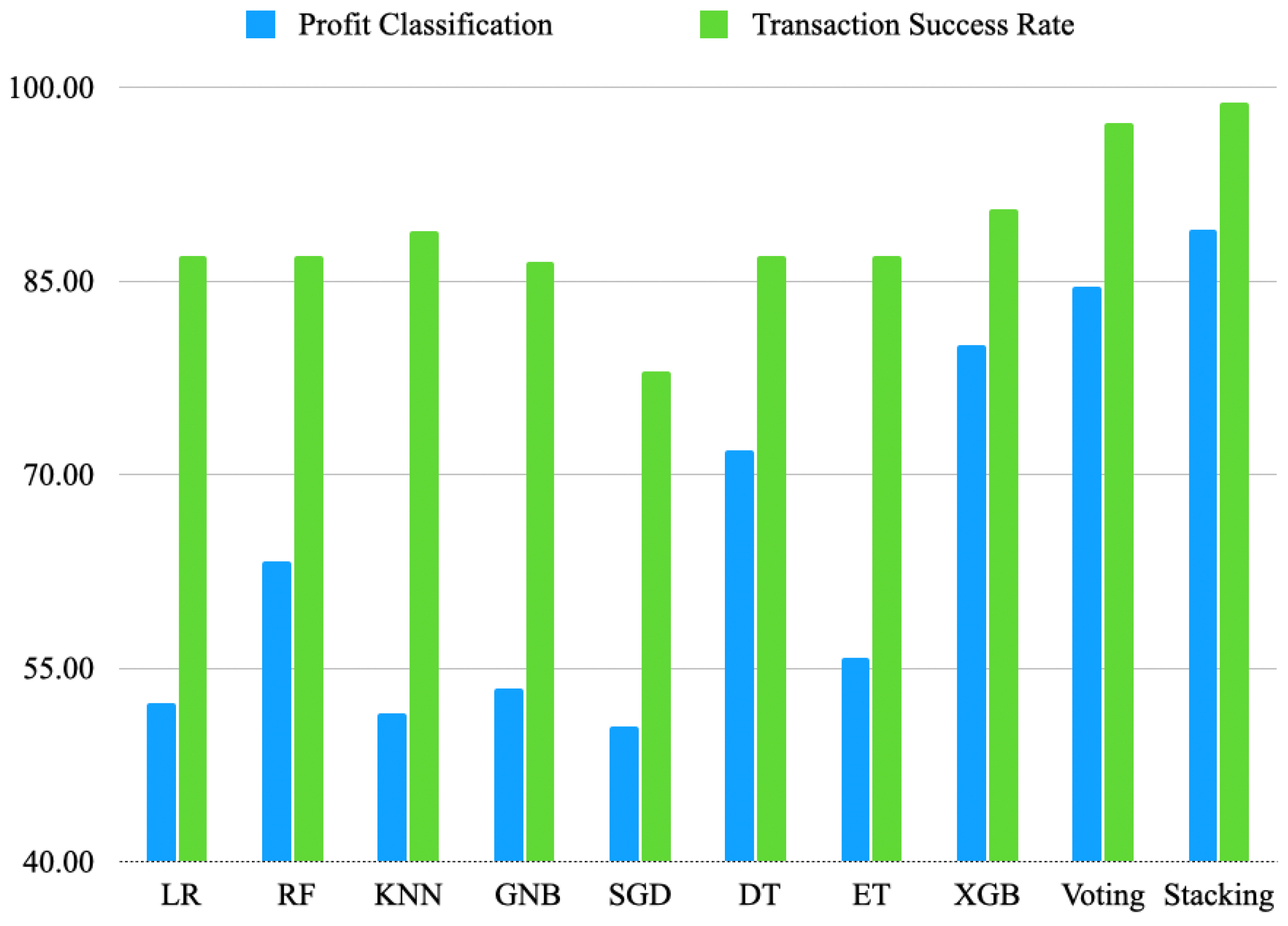
Each of these individual classifiers may have a unique approach or strategy for analyzing the dataset, which can be seen from from the results. However, simply taking the majority decision may not always be the best approach, because some classifiers may give more false-positives or true-negatives in classification c others. In such cases, it might be better to consider all the factors related to a classifier and the algorithm behind it before using it for predictions In a general sense, the WOA algorithm found a set of hyperparameters that increase the number of trees in the ensemble model, (n_estimators) and limit the depth of each tree (max_depth) to avoid overfitting. It also adjusts the learning rate (learning_rate) to optimize the trade-off between the speed of convergence and the accuracy of the model. Figure 12 shows the accuracies obtained by the models for both of our classification problems where we use whale optimization algorithms. The confusion matrices for the stacking classifier are shown in Figure 11 for both the tasks i.e., profit and success rate prediction.

The other classification system is used to determine if machine learning can predict success and failure rates along with the profits to cover another aspect of the real-world scenario for the cryptocurrency with good accuracy. In this case, we consider data such as sender, receiver, transaction type, status, amount and token type. The Status could be confirmed and unconfirmed in this case to address records as SUCCESS or FAILED (

Table 3. The average accuracy of the models over several runs for profit classification and transaction success rates.

Machine Learning Model	Profit Classification Accuracy (%)	Transaction Success Rate Classification Accuracy (%)
Logistic Regression (LR)	52.278	86.94
Random Forest (RF)	63.3	87
K-Nearest Neighbour (KNN)	51.502	87
Gaussian Naive Bayes (GNB)	53.433	86.5
Stochastic Gradient Descent	50.54	78.04
Decision Tree (DT)	71.89	86.93
Extra Tree (ET)	55.79	86.97
XGBoost (XGB)	80.042	90.54
Voting Classifier	84.55	97.21
Stacking Classifier	89.05	98.88

).

The proposed work focuses on enhancement in deployment mechanisms and superior optimization techniques to predict the success and failure of transactions in a TRON environment. All the reported values are mean values for 5 runs, and this is performed to ensure reduced bias of the models towards optimized solutions. One thing to note, however, is that it’s best to reset the environment after each run in order to reduce re-fitting towards optimal values in a particular run.

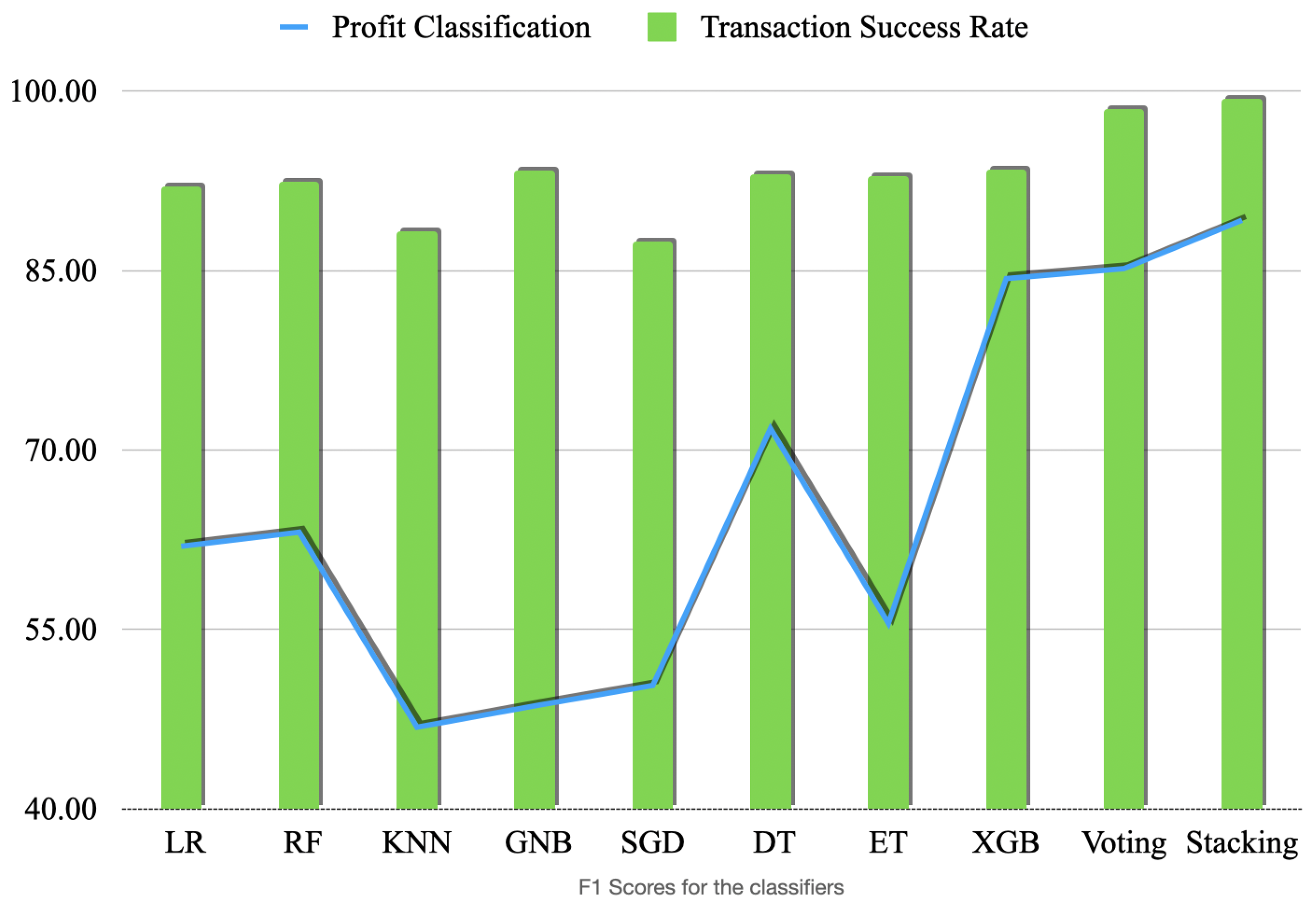
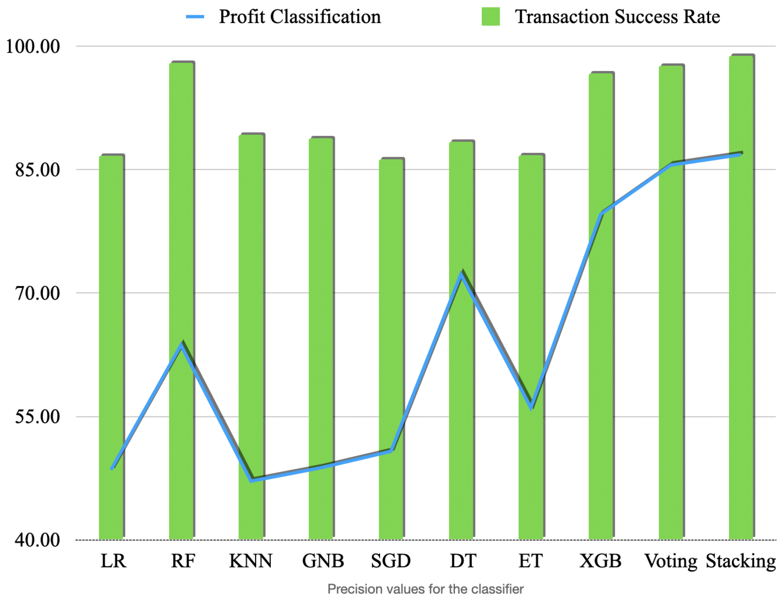
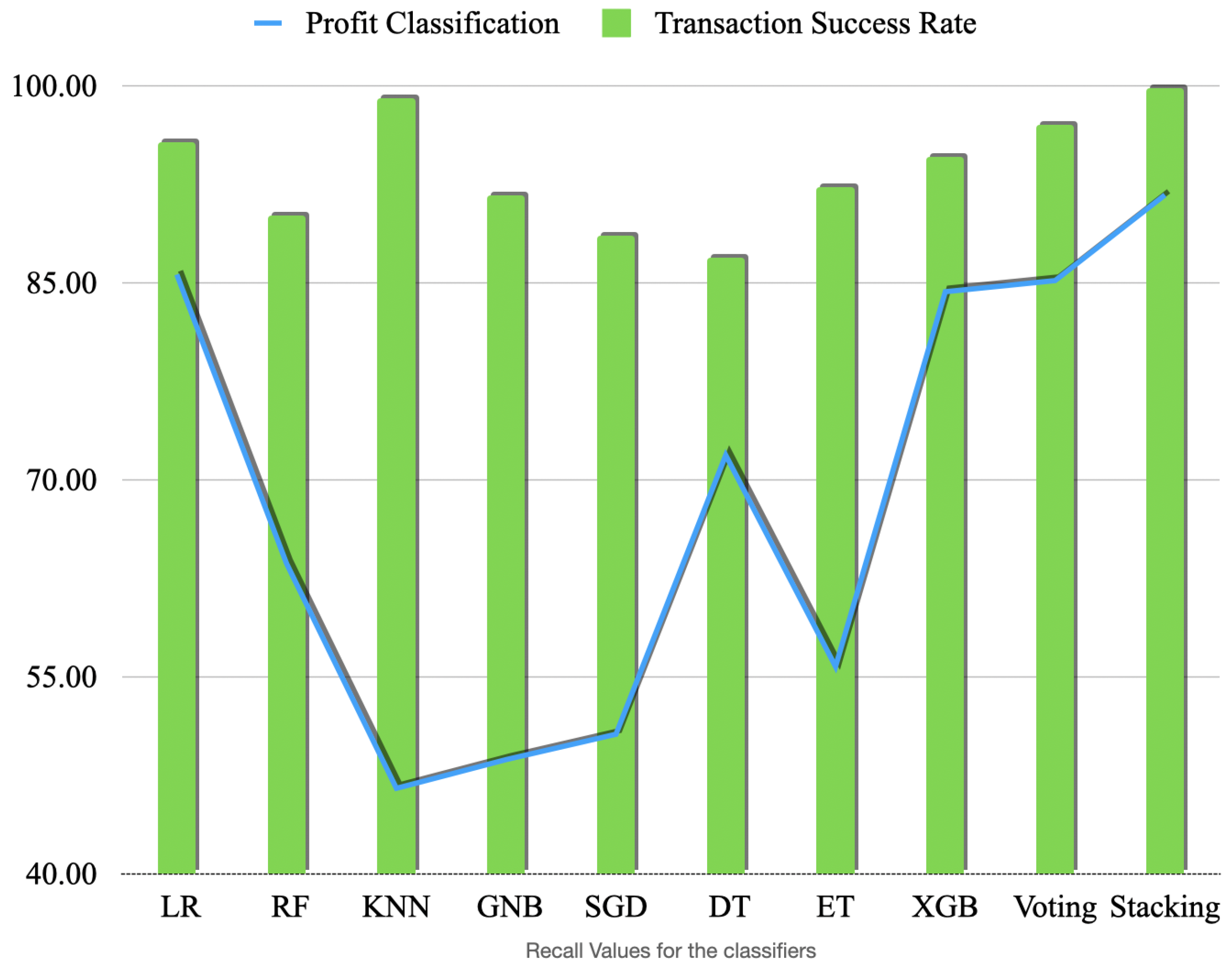
Figure 13, Figure 14 and Figure 15 show the F1, scores (the harmonic mean of precision and recall), precision and recall values, respectively. These scores show that some models consistently better than the others and have higher scores than the others for all the metrics. Stacking classifier has the best overall performance across all the metrics. Ensemble models should always be assessed for any overfitting at all times when used for unbalanced and smaller dataset and regularisation techniques that we applied are useful of avoiding overfitting to a certain extent.

There is very limited research on TRON to compare our results and specifically on the dataset that we use. It is concluded in the research work by Yadav et al. [47] in 2021 that TRON performs the best out of five cryptocurrencies in their analysis. Similarly, research by Malsa et al. [48] shows that theTRX coin has a promising future based on their qualitative and quantitative analysis of the parameters of the coin. From recent research performed for 10 different cryptocurrencies on a time-series dataset [49], TRON shows promising results compared to similar tokens, obtaining an MSE value ranging from 0.0007 to 0.0009, RMSE ranging from 0.0081 to 0.0094 and MAE value ranging from 0.0052 to 0.0061.

Our models perform better for most of the values, potentially due to a robust hyperparameter tuning methodology combined with using tree-based regressors which perform significantly better on smaller datasets [50]. It is important to note that even time series data may contain similar OHLC data that have significant overlap with our dataset. One important analysis from the literature on crypto price prediction is that the newer cryptocurrencies tend to show better performance when compared to their established counterparts in terms of MAE, R squared, and RSME values. Our findings show similar results and they reflect in other research works as well.

The models with the highest precision values for this binary classification problem are Stacking and Voting, with precision values ranging from 85.19% to 99.84%. Logistic Regression (LR) and XGBoost (XGB) also performed consistently well, achieving high precision values in addition to high overall accuracy.

Interestingly, LR and KNN show abnormally high values of recall for transaction success rate classification. Another possibility is that it is due to the imbalanced dataset itself, meaning that there are more negative cases than positive cases. One possibility is that the model is able to learn relevant patterns in the data that distinguish positive cases from negative cases. For example, in a binary classification problem, the model may learn to recognize specific features or combinations of features that are more likely to be present in positive cases. If these patterns are strong and consistent across the dataset, the model may be able to correctly identify a high proportion of the actual positive cases, leading to a high recall value.

For all the algorithms executed, a pipeline is created using StandardScaler(), PCA(), and the corresponding classifier. The StandardScaler is used to normalize the input data, and PCA is used for dimensionality reduction. The Stacking classifier takes the pipelines as input, and the final estimator is a Voting Classifier that takes the classifiers as input. In this case, the regression models are trying to predict the next closing price of TRON based on historical data. The input data includes various features (such as the opening price, high price, low price, and volume) from past trading periods, and the output is the next closing price of TRON.

Since we want to optimize the hyperparameters of the voting and stacking classifiers, we treat this as a continuous optimization problem. In the algorithm for optimal global position vector, the position of each agent represents a solution in the search space. The algorithm starts by initializing the population of agents randomly in the search space. Then, for each agent in the population, the position is updated based on the agent’s current position and the position of the best agent found so far. The updated equations for the position depends on the current iteration, which determines the type of search being performed (exploration or exploitation). The fitness of each agent is evaluated using the fitness function. If the fitness of an agent is better than the fitness of the best agent found so far, the best agent is updated. The step size is also updated in each iteration. The algorithm stops after a maximum number of iterations is reached, and the position of the best agent found is returned as the optimal solution.

For the regression, The XGBRegressor and LightGBM models use similar boosting algorithms but differ in their implementation. The XGBRegressor uses a pre-sorted algorithm to build trees, while the LightGBM uses a histogram-based algorithm. The CatBoostRegressor is another gradient-boosting model that uses ordered boosting and a random permutation to train the decision trees. Once trained, the models can be used to make predictions on new data (in this case, the test data) by taking in the input features and outputting a predicted closing price. The accuracy of the model is typically measured using a performance metric such as mean squared error or R-squared, which is best to use in our case. The hyperparameters that tuned for the XGBoost, LightGBM, and CatBoost regressors include but are not limited to the learning rate, number of estimators, maximum depth, gamma, subsample ratio, and regularization parameters. The search space for the WOA can be defined by setting the bounds for each hyperparameter to be tuned. The fitness function for the WOA is set to evaluate the performance of the model with the given hyperparameters. This is performed by training the model with the given hyperparameters and evaluating its performance on a validation set. The validation set can be used to prevent overfitting during hyperparameter tuning.

The voting classifier uses these XGB, LGBM, and CatBoost models for voting, with 6 other models as estimators. These models are: XGBClassifier with n_estimators = X[0] and max_depth = int(X[1]), CatBoostClassifier with learning_rate = X[2], and LGBMClassifier with learning_rate = X[3]. The three models are combined in an ensemble model using a VotingClassifier with a ‘soft’ voting strategy. The accuracy of the model is computed as the mean of the accuracy scores across all folds. The search space is defined as a NumPy array that contains four rows, each corresponding to one of the four hyper-parameters to optimize. A similar approach is used for the stacking classifier, while the final estimator used for the stacking classifier is the voting classifier. It is to be noted that for the problem of classification, the XGBoost model performs or another set of models does not influence the accuracy to a great length, however, to obtain the best possible accuracies, it is best to use the voting classifier as the final estimator. The first column of each row specifies the minimum value for the hyperparameter, and the second column specifies the maximum value. The WOA algorithm is run with the fitness_function and search_space defined above, as well as the number of agents and iterations specified. We used the Nvidia K80 GPU based on cloud for our evaluations on google cloud with 32 GB of usable ram. Three different models are created using the hyperparameters specified in the input parameter X. Limitations of our work include working on an unbalanced and small dataset. Future research should focus on improving the overall effectiveness and security of the framework

5. Conclusions

TRX is rapidly expanding and has a sizable pool of financial resources. For now, it is not possible to exactly predict how high TRON (TRX) will rise. Based on the price predictions, one can form an opinion about TRON’s future. The volatility of cryptocurrencies makes it difficult to predict significant price variations in the future. However, prediction models have been and will always be useful to predict prices to some extent. It is important to thoroughly examine the ’market microstructure’ of crypto exchanges. In the past few months, cryptocurrency exchanges have been the focus of some research and have several pressing issues that require further investigation. These approaches may not mean a better assessment of the market directly but may be useful in researching such cryptocurrencies. It is concluded that tree-based regressors combined with staking and voting ensembles techniques using tree-based models in their structure are a good combination for predicting the price and forming an opinion about the future performance of the cryptocurrency based on the historical performance of the tokens. This research is applicable in real-life scenarios and has a wide scope and possesses flexibility in predicting prices in the future as well where the data are limited to make accurate predictions using conventional models.