Proximal Point Algorithm with Euclidean Distance on the Stiefel Manifold

Abstract

In this paper, we consider the problem of minimizing a continuously differentiable function on the Stiefel manifold. To solve this problem, we develop a geodesic-free proximal point algorithm equipped with Euclidean distance that does not require use of the Riemannian metric. The proposed method can be regarded as an iterative fixed-point method that repeatedly applies a proximal operator to an initial point. In addition, we establish the global convergence of the new approach without any restrictive assumption. Numerical experiments on linear eigenvalue problems and the minimization of sums of heterogeneous quadratic functions show that the developed algorithm is competitive with some procedures existing in the literature.

1. Introduction

In this paper, we are interested in designing a proximal point procedure to solve the following optimization problem

$$\underset{X\in {\mathbb{R}}^{n \times p}}{min}\mathcal{F}\left(X\right),\mathrm{s}.\mathrm{t}.X^{\top }X=I_p,$$

(1)

where $\mathcal{F}:{\mathbb{R}}^{n \times p}\to \mathbb{R}$ is a continuously differentiable matrix function and $I_p\in {\mathbb{R}}^{p \times p}$ denotes the identity matrix. The feasible set of Problem (1), denoted by $St(n,p)=\{X\in {\mathbb{R}}^{n \times p}:X^{\top }X=I_p\}$, is known as the Stiefel manifold [1]. Actually, this set constitutes an embedded Riemannian sub-manifold of the Euclidean space ${\mathbb{R}}^{n \times p}$ with dimensions equal to $np-\frac{1}{2}p(p+1)$ (see [1]). Notice that (1) is a well-defined optimization problem because $St(n,p)$ is a compact set and $\mathcal{F}$ is a continuous function; therefore, the Weierstrass theorem ensures the existence of at least one global minimizer (and even a global maximizer) for $\mathcal{F}$ on the Stiefel manifold.

The orthogonality-constrained minimization problem (1) is widely applicable in many fields, such as the nearest low-rank correlation matrix problem [2,3], the linear eigenvalue problem [4,5,6], sparse principal component analysis [5,7], Kohn–Sham total energy minimization [4,6,8,9], low-rank matrix completion [10], the orthogonal Procrustes problem [8,11], maximization of sums of heterogeneous quadratic functions from statistics [4,12,13], the joint diagonalization problem [13], dimension reduction techniques in pattern recognition [14], and deep neural networks [15,16], among others.

In the Euclidean setting, given $f:{\mathbb{R}}^n\to \mathbb{R}\cup \{\infty \}$, a closed proper convex function, the proximal operator ${\mathtt{p}\mathtt{r}\mathtt{o}\mathtt{x}}_f:{\mathbb{R}}^n\to {\mathbb{R}}^n$ is defined by

$${\mathtt{p}\mathtt{r}\mathtt{o}\mathtt{x}}_f\left(x\right)=\arg \underset{y\in {\mathbb{R}}^n}{min}f\left(y\right)+\frac{1}{2\alpha }{\parallel y-x\parallel }_2^2,$$

(2)

where ${\parallel ·\parallel }_2$ is the standard norm of ${\mathbb{R}}^n$ and $\alpha >0$ is the proximal parameter [17].

The scalar $\alpha$ plays an important role controlling the magnitude by which the proximal operator sends the points towards the optimum values of f. In particular, larger values of $\alpha$ are related to mapped points near the optimum, while smaller values of this parameter promote a smaller movement to the minimum. It can design iterative optimization procedures that use the proximal operator to define the recursive update scheme. For example, the proximal minimization algorithm [17], minimizes the cost function f by consecutively applying the proximal operator ${\mathtt{p}\mathtt{r}\mathtt{o}\mathtt{x}}_f(·)$, similar to fixed-point methods, to some given initial vector $x_0\in {\mathbb{R}}^n$.

Several researchers have proposed generalizations of the proximal minimization algorithm in the Riemannian context. This kind of method was first considered in the Riemannian context by Ferreira and Oliveira [18] in the particular case of Hadamard manifolds. Papa Quiroz and Oliveira [19] adapted the proximal point method for quasiconvex functions and proved full convergence of the sequence $\left\{x_k\right\}$ to a minimizer over Hadamard manifolds. In addition, Souza and Oliveira [20] introduced a proximal point algorithm to minimize DC functions on Hadamard manifolds. Wang et. al. [21] established linear convergence and finite termination of this type of algorithm on Hadamard manifolds. For this same type of manifold, in [22], the authors proved global convergence of inexact proximal point methods. Recently, Almeida et. al. [23] developed a modified version of the proximal point procedure for minimization over Hadamard manifolds. For the specific case of optimization on the Stiefel manifold, in [7], the authors proposed a proximal gradient method to minimize the sum of two function $f\left(X\right)+g\left(X\right)$ over $St(n,p)$, where f is smooth and its gradient is Lipschitz continuous, and g is convex and Lipschitz continuous. Another proximal-type algorithm is proposed in [24], where the authors developed a proximal linearized augmented Lagrangian algorithm (PLAM) to solve (1). However, the PLAM algorithm does not build a feasible sequence of iterates, which differs from the rest of the Riemannian proposals.

To minimize a function $\mathcal{F}:\mathcal{M}\to \mathbb{R}$ defined on a Riemannian manifold $\mathcal{M}$, all the approaches presented in [18,19,20,21,23,25] consider the following generalization of (2)

$${\mathtt{p}\mathtt{r}\mathtt{o}\mathtt{x}}_{\mathcal{F}}\left(X\right)=\arg \underset{Y\in \mathcal{M}}{min}\mathcal{F}\left(Y\right)+\frac{1}{2\alpha }{\mathrm{dist}}^2(X,Y),$$

(3)

where $\mathrm{dist}(X,Y)$ is the Riemannian distance [1]. The main disadvantage of all these works is that the authors proposed methods and theoretical analyses based on the exponential mapping, which requires the construction of geodesics on $\mathcal{M}$. However, it is not always possible to find closed expressions for geodesics over a given Riemannian manifold, since geodesics are defined through a differential equation, [1,26]. Even in the case when we have available a closed formula for the corresponding geodesics on $\mathcal{M}$, the computational cost of calculating the exponential mapping over a matrix space is too high, which is an obstacle to solving large-scale problems.

In this paper, we introduce a very simple proximal point algorithm to tackle Stiefel-manifold-constrained optimization problems. The proposed approach replaces the term $\mathrm{dist}(X,Y)$ in (3) with the usual matrix distance ${\parallel X-Y\parallel }_F$ in order to avoid purely Riemannian concepts and techniques such as Riemannian distance and geodesics. The proposed iterative method tries to solve the optimization problem (1) by repeatedly applying our modified proximal operator to a given starting point. We prove (without imposing the Lipschitz continuity hypothesis) that our method converges to critical points of the restriction of the cost function to the Stiefel manifold. Our preliminary computational results suggest that our proposal presents competitive numerical performance against several feasible methods existing in the literature.

The rest of this manuscript is organized as follows. Section 2 summarizes a few well-known notations and concepts of linear algebra and Riemannian geometry that will be exploited in this paper. Afterwards, Section 3 introduces a new proximal point algorithm to deal with optimization problems with orthogonality constraints. Section 4 provides a concise convergence analysis for the proposed algorithm. Section 5 presents some illustrative numerical results, where we compare our approach with several state-of-the-art methods for the solution of linear eigenvalue problems and the minimization of sums of heterogeneous quadratic functions. Finally, the paper ends with a conclusion in Section 6.

2. Preliminaries

Throughout this paper, we say that $W\in {\mathbb{R}}^{n \times n}$ is skew-symmetric if $W=-W^{\top }$. Given a square matrix $A\in {\mathbb{R}}^{m \times m}$, $\mathrm{skew}\left(A\right)$ denotes the skew-symmetric part of A; that is, $\mathrm{skew}\left(A\right)=0.5(A-A^{\top })$. The trace of X is defined as the sum of the diagonal elements, which we denote as $Tr\left[X\right]$. The standard inner product between two matrices $A,B\in {\mathbb{R}}^{m \times n}$ is given by $\langle A,B\rangle \equiv {\sum }_{i,j}{a}_{ij}{b}_{ij}=Tr\left[A^{\top }B\right]$. The Frobenius norm is defined by ${\parallel A\parallel }_F=\sqrt{\langle A,A\rangle }$. Let $X\in St(n,p)$ be an arbitrary matrix in the Stiefel manifold; the tangent space of the Stiefel manifold at X is given by [1]

$$T_{X}St(n,p)=\{Z\in {\mathbb{R}}^{n \times p}:Z^{\top }X+X^{\top }Z=0\}.$$

Let $X\in St(n,p)$; the canonical metric [6] associated with the tangent space of the Stiefel manifold is defined by

$${\langle {\xi }_X,{\eta }_X\rangle }_c\equiv Tr\left[{\xi }_X^{\top }\left(I-\frac{1}{2}X{X}^{\top }\right){\eta }_X\right],\forall {\xi }_X,{\eta }_X\in T_{X}St(n,p).$$

Let $\mathcal{F}:{\mathbb{R}}^{n \times p}\to \mathbb{R}$ be a differentiable function; we denote as $\mathcal{DF}\left(X\right)\equiv \left(\frac{\partial \mathcal{F}\left(X\right)}{\partial X_{ij}}\right)$ the matrix of partial derivatives of $\mathcal{F}$ (the Euclidean gradient of $\mathcal{F}$). Let $\Phi :St(n,p)\to \mathbb{R}$ be a smooth function defined on the Stiefel manifold; then the Riemannian gradient of $\Phi$ at $X\in St(n,p)$, denoted as $\nabla \Phi \left(X\right)$, is the unique vector in $T_{X}St(n,p)$ satisfying

$$\mathcal{D}\Phi \left(X\right)\left[{\xi }_X\right]:=\underset{\tau \to 0}{lim}\frac{\Phi \left(\gamma \right(\tau \left)\right)-\Phi \left(\gamma \right(0\left)\right)}{\tau }=\langle \nabla \Phi \left(X\right),{\xi }_X\rangle ,\forall {\xi }_X\in T_{X}St(n,p),$$

(4)

where $\gamma :[0,{\tau }_{max}]\to St(n,p)$ is any curve that verifies $\gamma \left(0\right)=X$ and $\dot{\gamma }\left(0\right)={\xi }_X$.

The Riemannian gradient of $\Phi :St(n,p)\to \mathbb{R}$ under the canonical metric has the following closed expression [4,6]

$$\nabla \Phi \left(X\right)=\mathcal{D}\Phi \left(X\right)-X\mathcal{D}\Phi {\left(X\right)}^{\top }X,\forall X\in St(n,p).$$

(5)

In addition, based on Formula (5), we can define the following projection operator over $T_{X}St(n,p)$

$$P_X^c\left[Z\right]=Z-X{Z}^{\top }X,\mathrm{with}Z\in {\mathbb{R}}^{n \times p}.$$

(6)

It can be easily shown that the operator (6) effectively projects matrices from ${\mathbb{R}}^{n \times p}$ to the tangent space $T_{X}St(n,p)$. This projection operator was also considered in [27].

Similar to the case of smooth unconstrained optimization, $X\in St(n,p)$ is a critical point of $\Phi :St(n,p)\to \mathbb{R}$ if it satisfies [1,28]

$$\nabla \Phi \left(X\right)=0.$$

Therefore, the critical points of the restriction of the cost function $\mathcal{F}$ to the Stiefel manifold are candidates to be local minimizers of Problem (1). Here, we clarify that the objective function $\mathcal{F}$ that appears in (1) has both a Euclidean gradient and a Riemannian gradient. In the rest of this paper, we will denote by $\nabla \mathcal{F}(·)$ the Riemannian gradient of the restriction of $\mathcal{F}$ to the set $St(n,p)$ under the canonical metric.

3. Proximal Point Algorithm on $\mathit{St}(\mathit{n},\mathit{p})$

In this section, we propose an implicitly defined curve on the Stiefel manifold. We also validate that the proposed curve verifies analogous properties that Riemannian gradient methods have. Using this curve, we further present in detail the proposed proximal point algorithm.

As we mentioned in the introduction, we consider an adaptation of the exact proximal point method to the framework of minimization over the Stiefel manifold: given a feasible point $X\in St(n,p)$, we compute the new iterate $X\left(\overline{\alpha }\right)$ as a point on the curve $X(·):[0,{\alpha }_{max}]\to St(n,p)$ defined by

$$X\left(\alpha \right)\equiv \arg \underset{Y\in {\mathbb{R}}^{n \times p}}{min}\alpha \mathcal{F}\left(Y\right)+\frac{1}{2}{\parallel Y-X\parallel }_F^2,\mathrm{s}.\mathrm{t}.Y^{\top }Y=I_p.$$

(7)

Observe that the argmin set in (7) is never empty since $\alpha \mathcal{F}\left(Y\right)+\frac{1}{2}{\parallel Y-X\parallel }_F^2$ is a continuous function on a compact domain. In addition, note that this proximal optimization problem is obtained from (3) by substituting the Riemannian distance with the standard metric associated with the matrix space ${\mathbb{R}}^{n \times p}$. Additionally, $X\left(\alpha \right)$ satisfies that $X\left(0\right)=X$. Thus, $X\left(\alpha \right)$ is a curve on $St(n,p)$ that connects the consecutive iterates X and $X\left(\overline{\alpha }\right)$. This is an analogous property to that which the retraction-based line-search curves verify (see [1,29]). Here it is important to remark that (7) can have multiple global solutions; in this situation, $X\left(\alpha \right)$ would not be a curve since it would not be a well-defined function.

The lemma below establishes that $X\left(\alpha \right)$ is a descent iterative process.

Lemma 1.

Given $X\in St(n,p)$, consider the curve (7). Then,

$$\mathcal{F}\left(X\left(\alpha \right)\right)\le \mathcal{F}\left(X\right)-\frac{1}{2\alpha }{\parallel X\left(\alpha \right)-X\parallel }_F^2,\forall \alpha \in (0,\infty ).$$

(8)

Proof of Lemma 1.

Let $\alpha$ be a positive real number. In view of the optimality of $X\left(\alpha \right)$ in (7), we have

$$\alpha \mathcal{F}\left(X\left(\alpha \right)\right)+\frac{1}{2}{\parallel X\left(\alpha \right)-X\parallel }_F^2\le \alpha \mathcal{F}\left(X\right).$$

(9)

Post-multiplying both sides of (9) by ${\alpha }^{-1}$ and rearranging, we obtain

$$\mathcal{F}\left(X\left(\alpha \right)\right)\le \mathcal{F}\left(X\right)-\frac{1}{2\alpha }{\parallel X\left(\alpha \right)-X\parallel }_F^2,$$

completing the poof.    □

Lemma 1 guarantees that the proposed approach is a descent iterative process. Therefore, by executing an iterative process based on the proximal curve (7), we can minimize the objective function and at the same time move towards stationarity. Taking into account this fact, we propose our proximal point algorithm on $St(n,p)$, the steps for which are described in Algorithm 1 (PPA-St).

Algorithm 1 PPA-St

1: $X_0\in St(n,p)$, $0<{\alpha }_{min}\le {\alpha }_{max}<\infty$, $\left\{{\alpha }_k\right\}$ is a sequence such that ${\alpha }_k\in [{\alpha }_{min},{\alpha }_{max}]$ for all $k\in \mathbb{N}$, $k\leftarrow 0$. 2: while $\parallel \nabla \mathcal{F}\left(X_k\right){\parallel }_F\ne 0$ do 3: $$X_{k+1}=\arg \underset{Y\in St(n,p)}{min}{\alpha }_k\mathcal{F}\left(Y\right)+\frac{1}{2}{\parallel Y-X_k\parallel }_F^2.$$ (10) 4:    If $\parallel X_{k+1}-X_k{\parallel }_F =0$ then stop the algorithm. 5:    $k\leftarrow k+1$, 6: end while

Notice that the proposed PPA-St algorithm can be interpreted as a Euclidean proximal point algorithm with respect to the cost function

$$f\left(X\right)=F\left(X\right)+{\delta }_{St(n,p)}\left(X\right),$$

where ${\delta }_{St(n,p)}$ is the indicator function given by

$${\delta }_{St(n,p)}\left(X\right)=\left\{\begin{array}{cc}0\hfill & \mathrm{if} X\in \mathrm{St}(n,p)\hfill \\ +\infty \hfill & \mathrm{otherwise},\hfill \end{array}\right.$$

and $F:{\mathbb{R}}^{n \times p}\to (-\infty ,+\infty ]$ is defined by

$$F\left(X\right)=\left\{\begin{array}{cc}\mathcal{F}\left(X\right)\hfill & \mathrm{if} X\in \mathrm{St}(n,p)\hfill \\ +\infty \hfill & \mathrm{otherwise}.\hfill \end{array}\right.$$

Thus the PPA-St process can be seen as a special case of the proximal alternating linearized descent (PALM) algorithm developed in [30] by selecting the functions $H(x,y)=0$ and $g\left(y\right)=0$ (in the notation of [30]). Particularly, PALM has a rich convergence analysis and was already applied to the Stiefel manifold in [31,32]. Nonetheless, the main differences between PALM and PPA-St are that our proposal does not require linearizing the function $F(·)$ to solve the problem, and PPA-St does not involve inertial steps.

On the other hand, there are some cost functions for which the proxy (7) can be solved analytically. For example, if ${\mathcal{F}}_1\left(Y\right)=Tr\left[Y^{\top }M\right]$, where $M\in {\mathbb{R}}^{n \times p}$ is a data matrix, then the proximity operators are

$$X\left(\alpha \right)\equiv \arg \underset{Y\in {\mathbb{R}}^{n \times p}}{min}\alpha Tr\left[Y^{\top }M\right]+\frac{1}{2}{\parallel Y-X\parallel }_F^2,\mathrm{s}.\mathrm{t}.Y^{\top }Y=I_p.$$

(11)

with $X\in St(n,p)$ constant. Since $X,Y\in St(n,p)$, the optimization problem above is equivalent to

$$X\left(\alpha \right)\equiv \arg \underset{Y\in {\mathbb{R}}^{n \times p}}{min}\frac{1}{2}{\parallel Y-(X-\alpha M)\parallel }_F^2,\mathrm{s}.\mathrm{t}.Y^{\top }Y=I_p,$$

(12)

which has a closed-form solution (see Proposition 2.3 in [8]). Additionally, let $A,B\in {\mathbb{R}}^{n \times n}$ be two constant matrices and $X\in St(n,n)$. Let us consider the objective function ${\mathcal{F}}_2:{\mathbb{R}}^{n \times n}\to \mathbb{R}$ given by ${\mathcal{F}}_2\left(Y\right)=\frac{1}{2}{\parallel AY-B\parallel }_F^2$. In this special case, the proximal operator is reduced to

$$X\left(\alpha \right)\equiv \arg \underset{Y\in {\mathbb{R}}^{n \times n}}{min}\frac{\alpha }{2}{\parallel AY-B\parallel }_F^2+\frac{1}{2}{\parallel Y-X\parallel }_F^2,\mathrm{s}.\mathrm{t}.Y^{\top }Y=I_n.$$

(13)

The above constrained optimization problem can be reformulated as

$$X\left(\alpha \right)=\arg \underset{Y\in {\mathbb{R}}^{n \times n}}{min}\frac{1}{2}\parallel \left[\genfrac{}{}{0pt}{}{A}{(1/\sqrt{\alpha })I}\right]Y-\left[\genfrac{}{}{0pt}{}{B}{(1/\sqrt{\alpha })X}\right]{\parallel }_F^2\mathrm{s}.\mathrm{t}.Y^{\top }Y=I_n,$$

(14)

which is an orthogonal Procrustes problem with an analytical solution (see [33]). However, in general the proximal operator (7) does not have a closed-form expression for its solutions. Therefore, in the implementation of PPA-St, we will use an efficient Riemannian gradient method based on the QR-retraction mapping (see Example 4.1.3 in [1]) in order to solve the optimization subproblem (10).

By introducing the notation ${\varphi }_k\left(Y\right)\equiv {\alpha }_k\mathcal{F}\left(Y\right)+\frac{1}{2}{\parallel Y-X_k\parallel }_F^2$, we propose to use the following feasible line-search method, starting at $Y_0^k=X_k$ and ${\tau }_0={\alpha }_k$,

$$Y_{i+1}^k=(Y_i^k-{\tau }_i\nabla {\varphi }_k\left(Y_i^k\right))\mathtt{c}\mathtt{h}\mathtt{o}\mathtt{l}{(I_p+{\tau }_i^2\nabla {\varphi }_k{\left(Y_i^k\right)}^{\top }\nabla {\varphi }_k\left(Y_i^k\right))}^{-1},$$

(15)

where $\nabla {\varphi }_k\left(Y\right)$ is the Riemannian gradient under the canonical metric of ${\varphi }_k$ evaluated at Y; that is, $\nabla {\varphi }_k\left(Y\right)=P_Y^c\left[\mathcal{D}{\varphi }_k\left(Y\right)\right]$, where $\mathcal{D}{\varphi }_k\left(Y\right)$ is the Euclidean gradient of ${\varphi }_k$, i.e., $\mathcal{D}{\varphi }_k\left(Y\right)={\alpha }_k\mathcal{DF}\left(Y\right)+Y-X_k$. In addition, $\mathtt{c}\mathtt{h}\mathtt{o}\mathtt{l}\left(A\right)$ denotes the Cholesky factor obtained from the Cholesky factorization of $A\in {\mathbb{R}}^{p \times p}$, i.e., let $A\in {\mathbb{R}}^{p \times p}$ be a symmetric and positive definite matrix (PSD) and suppose that $A=L_A^{\top }{L}_A$ is its Cholesky decomposition; then $\mathtt{c}\mathtt{h}\mathtt{o}\mathtt{l}\left(A\right)\equiv L_A$. Observe that this function is well-defined due to the uniqueness of Cholesky factorization for PSD matrices. Additionally, notice that in the recursive scheme (15), we are projecting $Y_i^k-{\tau }_i\nabla {\varphi }_k\left(Y_i^k\right)$ over the Stiefel manifold using its QR factorization obtained from the Cholesky decomposition (see Equation (1.3) in [34]). We now present the inexact version of our Algorithm 1 based on the Riemannian gradient scheme (15).

It is well-known that if we endow the iterative method (15) with a globalization strategy to determine the step-size ${\tau }_i>0$, such as the Armijo’s rule [1,35] or a non-monotone Zhang–Hager type condition [36,37], then the Riemannian line-search method (15) is globally convergent (please see [1,36]). This means that the while loop between Steps 3 and 6 of Algorithm 2 does not take infinite time, i.e., there must exist an index ${\mathcal{I}}_k\in \mathbb{N}$ such that $\parallel \nabla {\varphi }_k\left(Y_i^k\right){\parallel }_F\le {\epsilon }_k$ for all $i\ge {\mathcal{I}}_k$. In addition, it is always possible to determine a step-size ${\tau }_i>0$ such that Armijo’s rule (16) holds. For practical purposes, we implement our Algorithm 2 using the well-known backtracking strategy to find such a step-size (see [35]). Furthermore, to reduce the number of line searches performed in each inner iteration (the iterations in terms of the index i), we incorporate the Barzilai–Borwein step-size, which typically improves the performance of gradient-type methods (see [38]).

Algorithm 2 Inexact PPA-St

1: $X_0\in St(n,p)$, $0<{\alpha }_{min}\le {\alpha }_{max}<\infty$, $c_1\in (0,1)$, $\left\{{\alpha }_k\right\}$ is a sequence such that ${\alpha }_k\in [{\alpha }_{min},{\alpha }_{max}]$ for all $k\in \mathbb{N}$, $\left\{{\epsilon }_k\right\}$ is a sequence of positive real numbers such that ${\epsilon }_k\to 0$, $k\leftarrow 0$. 2: while $\parallel \nabla \mathcal{F}\left(X_k\right){\parallel }_F\ne 0$ do 3:    Set $Y_0^k=X_0$ and $i=0$. 4:    while $\parallel \nabla {\varphi }_k\left(Y_i^k\right){\parallel }_F>{\epsilon }_k$ do 5:      $Y_{i+1}^k=(Y_i^k-{\tau }_i\nabla {\varphi }_k\left(Y_i^k\right))\mathtt{c}\mathtt{h}\mathtt{o}\mathtt{l}{(I_p+{\tau }_i^2\nabla {\varphi }_k{\left(Y_i^k\right)}^{\top }\nabla {\varphi }_k\left(Y_i^k\right))}^{-1}$,      where ${\tau }_i>0$ is selected in such a way that the Armijo condition is satisfied, i.e., $${\varphi }_k\left(Y_{i+1}^k\right)\le {\varphi }_k\left(Y_i^k\right)-c_1{\tau }_i{\parallel \nabla {\varphi }_k\left(Y_i^k\right)\parallel }_F^2,$$ (16) 6:      $i\leftarrow i+1$, 7:    end while 8:    $X_{k+1}=Y_i^k$, 9:    $k\leftarrow k+1$, 10: end while

4. Convergence Results

In this section, we establish the global convergence of Algorithms 1 and 2. Here, we say that an algorithm is globally convergent if, for any initial point $X_0\in St(n,p)$, the generated sequence $\left\{X_k\right\}$ satisfies that $\nabla \mathcal{F}\left(X_k\right)\to 0$. Thus, global convergence does not refer to convergence towards global optima. Firstly, we analyze the convergence properties of Algorithm 1 by revealing the relationships between the residuals $\parallel \nabla \mathcal{F}\left(X_k\right){\parallel }_F$, $\mid \mathcal{F}\left(X_{k+1}\right)-\mathcal{F}\left(X_k\right)\mid$ and $\parallel X_{k+1}-X_k{\parallel }_F$.

Since $\mathcal{F}$ is continuously differentiable over ${\mathbb{R}}^{n \times p}$, then its derivative $\mathcal{DF}\left(X\right)$ is continuous. Hence, $\mathcal{DF}\left(X\right)$ is bounded on $St(n,p)$ due to the compactness of the Stiefel manifold. Then, there exists a constant $\kappa >0$ such that

$${\parallel \mathcal{DF}\left(X\right)\parallel }_F\le \kappa ,\forall X\in St(n,p).$$

(17)

Consequently, the Riemannian gradient of $\mathcal{F}$ satisfies

$${\parallel \nabla \mathcal{F}\left(X\right)\parallel }_F={\parallel \mathcal{DF}\left(X\right)-X\mathcal{DF}{\left(X\right)}^{\top }X\parallel }_F\le 2\kappa ,$$

(18)

for all $X\in St(n,p)$.

The following proposition states that Algorithm 1 stops at Riemannian critical points of $\mathcal{F}$.

Proposition 1.

Let $\left\{X_k\right\}$ be a sequence generated by Algorithm 1. Suppose that Algorithm terminates at iteration $k\in \mathbb{N}$; then $\nabla \mathcal{F}\left(X_k\right)=0$.

Proof of Proposition 1.

The first-order necessary optimality condition associated with Subproblem (10) leads to

$${\alpha }_k\nabla \mathcal{F}\left(X_{k+1}\right)+P_{X_{k+1}}^c[X_{k+1}-X_k]=0,$$

(19)

but since Algorithm 1 terminates at the k-th iteration, we have that $X_{k+1}=X_k$, which directly implies that $P_{X_{k+1}}^c[X_{k+1}-X_k]=P_{X_{k+1}}^c\left[0\right]=0$. By substituting this fact in (19), we obtain the desired result. □

The rest of this section is devoted to study the asymptotic behavior of Algorithm 1 for infinite sequences $\left\{X_k\right\}$ generated by our approach, since otherwise, Proposition 1 says that Algorithm 1 returns a stationary point for Problem (1). The lemma below provides us two key theoretical results.

Lemma 2.

Let $\left\{X_k\right\}$ be an infinite sequence generated by Algorithm 1. Then, we have

1.

$\left\{\mathcal{F}\left(X_k\right)\right\}$ is a convergent sequence.

2.

The residual sequence $\{\parallel X_{k+1}-X_k{\parallel }_F\}$ converges to zero.

Proof of Lemma 2.

It follows from Lemma 1 that

$$\mathcal{F}\left(X_k\right)\le \mathcal{F}\left(X_{k-1}\right)-\frac{1}{2{\alpha }_{k-1}}{\parallel X_k-X_{k-1}\parallel }_F^2.$$

(20)

Therefore, $\left\{\mathcal{F}\left(X_k\right)\right\}$ is a monotonically decreasing sequence. Now, since the Stiefel manifold is a compact set and $\mathcal{F}$ is a continuous function, we obtain that $\mathcal{F}$ has a maximum and minimum on $St(n,p)$. Therefore, $\left\{\mathcal{F}\left(X_k\right)\right\}$ is bounded, and then $\left\{\mathcal{F}\left(X_k\right)\right\}$ is a convergent sequence, which proves the first part of the lemma.

On the other hand, by rearranging Inequality (20), we arrive at

$$\begin{array}{ccc}\hfill \parallel X_k-X_{k-1}{\parallel }_F^2& \le & 2{\alpha }_{k-1}\left(\mathcal{F}\left(X_{k-1}\right)-\mathcal{F}\left(X_k\right)\right)\hfill \\ & \le & 2{\alpha }_{max}\left(\mathcal{F}\left(X_{k-1}\right)-\mathcal{F}\left(X_k\right)\right).\hfill \end{array}$$

(21)

Applying limits in (21) and using the first part of this lemma, we obtain

$$\underset{k\to \infty }{lim}{\parallel X_{k+1}-X_k\parallel }_F=0.$$

□

Now we are ready to prove the global convergence of Algorithm 1, which is established in the theorem below.

Theorem 1.

Let $\left\{X_k\right\}$ be an infinite sequence generated by Algorithm 1. Then

$$\underset{k\to \infty }{lim}{\parallel \nabla \mathcal{F}\left(X_{k+1}\right)\parallel }_F=0.$$

Proof of Theorem 1.

Firstly, let us denote by $P_k:=X_{k+1}{(X_{k+1}-X_k)}^{\top }{X}_{k+1}$. Now, notice that

$$\parallel P_k{\parallel }_F=\parallel X_{k+1}{(X_{k+1}-X_k)}^{\top }{X}_{k+1}{\parallel }_F\le {\parallel X_{k+1}-X_k\parallel }_F.$$

(22)

By applying Lemma 2 in (22), we obtain

$$\underset{k\to \infty }{lim}{\parallel P_k\parallel }_F=0.$$

(23)

From Lemma 1, we have

$$\mathcal{F}\left(X_{k+1}\right)\le \mathcal{F}\left(X_k\right)-\frac{1}{2{\alpha }_k}{\parallel X_{k+1}-X_k\parallel }_F^2.$$

(24)

It follows from (24), (7), the Cauchy–Schwarz inequality, and (18) that

$$\begin{array}{ccc}\hfill \mathcal{F}\left(X_{k+1}\right)& \le & \mathcal{F}\left(X_k\right)-\frac{1}{2{\alpha }_k}{\parallel X_{k+1}-X_k\parallel }_F^2\hfill \\ & =& \mathcal{F}\left(X_k\right)-\frac{1}{2{\alpha }_k}{\parallel P_k-{\alpha }_k\nabla \mathcal{F}\left(X_{k+1}\right)\parallel }_F^2\hfill \\ & =& \mathcal{F}\left(X_k\right)-\frac{1}{2{\alpha }_k}\parallel P_k{\parallel }_F^2+Tr[P_k^{\top }\nabla \mathcal{F}\left(X_{k+1}\right)]-\frac{{\alpha }_k}{2}{\parallel \nabla \mathcal{F}\left(X_{k+1}\right)\parallel }_F^2\hfill \\ & <& \mathcal{F}\left(X_k\right)+Tr[P_k^{\top }\nabla \mathcal{F}\left(X_{k+1}\right)]-\frac{{\alpha }_k}{2}{\parallel \nabla \mathcal{F}\left(X_{k+1}\right)\parallel }_F^2\hfill \\ & \le & \mathcal{F}\left(X_k\right)+Tr[P_k^{\top }\nabla \mathcal{F}\left(X_{k+1}\right)]-\frac{{\alpha }_{min}}{2}{\parallel \nabla \mathcal{F}\left(X_{k+1}\right)\parallel }_F^2\hfill \\ & \le & \mathcal{F}\left(X_k\right)+2\kappa \parallel P_k{\parallel }_F-\frac{{\alpha }_{min}}{2}{\parallel \nabla \mathcal{F}\left(X_{k+1}\right)\parallel }_F^2,\hfill \end{array}$$

(25)

which implies that

$$\parallel \nabla \mathcal{F}\left(X_{k+1}\right){\parallel }_F^2\le \frac{2}{{\alpha }_{min}}\left(\mathcal{F}\left(X_k\right)-\mathcal{F}\left(X_{k+1}\right)\right)+\frac{4\kappa }{{\alpha }_{min}}{\parallel P_k\parallel }_F.$$

(26)

Finally, taking limits in (26) and considering (23) and Lemma 2, we obtain

$$\underset{k\to \infty }{lim}{\parallel \nabla \mathcal{F}\left(X_{k+1}\right)\parallel }_F=0,$$

which completes the proof. □

We now turn to proving the convergence to stationary points of the inexact version of the PPA-St approach.

Theorem 2.

Let $\left\{X_k\right\}$ be an infinite sequence generated by Algorithm 2. Then

$$\underset{k\to \infty }{lim}{\parallel \nabla \mathcal{F}\left(X_{k+1}\right)\parallel }_F=0.$$

Proof of Theorem 2.

From the Armijo condition (16), Step 7, and the definition of ${\varphi }_k\left(Y\right)$, we have

$${\alpha }_k\mathcal{F}\left(X_{k+1}\right)+\frac{1}{2}\parallel X_{k+1}-X_k{\parallel }_F^2\le {\varphi }_k\left(Y_{i-1}^k\right)-c_1{\tau }_{i-1}{\parallel \nabla {\varphi }_k\left(Y_{i-1}^k\right)\parallel }_F^2.$$

(27)

Additionally, the Armijo condition (16) clearly implies that, for fixed k, $\left\{{\varphi }_k\left(Y_i^k\right)\right\}$ is a non-increasing sequence. Combining this result with inequality (27) and Step 2, we arrive at

$$\begin{array}{ccc}\hfill {\alpha }_k\mathcal{F}\left(X_{k+1}\right)+\frac{1}{2}{\parallel X_{k+1}-X_k\parallel }_F^2& \le & {\varphi }_k\left(Y_{i-1}^k\right)-c_1{\tau }_{i-1}{\parallel \nabla {\varphi }_k\left(Y_{i-1}^k\right)\parallel }_F^2\hfill \\ & \le & {\varphi }_k\left(Y_{i-1}^k\right)\hfill \\ & \le & {\varphi }_k\left(Y_0^k\right)={\alpha }_k\mathcal{F}\left(X_k\right),\hfill \end{array}$$

which leads to

$$\mathcal{F}\left(X_{k+1}\right)\le \mathcal{F}\left(X_k\right)-\frac{1}{2{\alpha }_k}{\parallel X_{k+1}-X_k\parallel }_F^2.$$

Therefore, the sequence of objective values $\left\{\mathcal{F}\left(X_k\right)\right\}$ is convergent. Moreover, we get that ${lim}_{k\to \infty }{\parallel X_{k+1}-X_k\parallel }_F^2=0$.

On the other hand, notice that

$$\nabla {\varphi }_k\left(X_{k+1}\right)={\alpha }_k\nabla \mathcal{F}\left(X_{k+1}\right)+P_{X_k}^c[X_{k+1}-X_k].$$

(28)

The second term on the right-hand side of (28) verifies that

$$\begin{array}{ccc}\hfill \left|\right|P_{X_k}^c[X_{k+1}-X_k]{\left|\right|}_F& =& \parallel (X_{k+1}-X_k)-X_k{(X_{k+1}-X_k)}^{\top }{X}_k{\parallel }_F\hfill \\ & \le & \parallel X_{k+1}-X_k{\parallel }_F+{\parallel X_k{(X_{k+1}-X_k)}^{\top }{X}_k\parallel }_F\hfill \\ & \le & \parallel X_{k+1}-X_k{\parallel }_F+\parallel X_k{\parallel }_F^2{\parallel X_{k+1}-X_k\parallel }_F\hfill \\ & =& \left(1+\parallel X_k{\parallel }_F^2\right){\parallel X_{k+1}-X_k\parallel }_F\hfill \\ & =& \left(1+Tr\left[X_k^{\top }{X}_k\right]\right){\parallel X_{k+1}-X_k\parallel }_F\hfill \\ & =& \left(1+Tr\left[I_p\right]\right){\parallel X_{k+1}-X_k\parallel }_F\hfill \\ & =& (1+p)\parallel X_{k+1}-X_k{\parallel }_F.\hfill \end{array}$$

(29)

By rearranging (28), we get

$$\nabla \mathcal{F}\left(X_{k+1}\right)=\frac{1}{{\alpha }_k}\left(\nabla {\varphi }_k\left(X_{k+1}\right)-P_{X_k}^c[X_{k+1}-X_k]\right).$$

Applying the norm to both sides of the above equality and considering that $\parallel \nabla {\varphi }_k\left(X_{k+1}\right){\parallel }_F$$\le {\epsilon }_k$ and (29), we arrive at

$$\begin{array}{ccc}\hfill \parallel \nabla \mathcal{F}\left(X_{k+1}\right){\parallel }_F& \le & \frac{1}{{\alpha }_k}{\parallel \nabla {\varphi }_k\left(X_{k+1}\right)-P_{X_k}^c[X_{k+1}-X_k]\parallel }_F\hfill \\ & \le & \frac{1}{{\alpha }_{min}}\left(\parallel \nabla {\varphi }_k\left(X_{k+1}\right){\parallel }_F+{\parallel P_{X_k}^c[X_{k+1}-X_k]\parallel }_F\right)\hfill \\ & \le & \frac{1}{{\alpha }_{min}}\left({\epsilon }_k+(1+p){\parallel X_{k+1}-X_k\parallel }_F\right).\hfill \end{array}$$

Taking limits in the above relation, we conclude that

$$\underset{k\to \infty }{lim}{\parallel \nabla \mathcal{F}\left(X_{k+1}\right)\parallel }_F=0,$$

proving the theorem. □

Corollary 1.

Let $\left\{X_k\right\}$ be an infinite sequence of iterates generated by Algorithm 1 or Algorithm 2. Then every accumulation point of $\left\{X_k\right\}$ is a critical point of $\mathcal{F}$ in the Riemannian sense.

Proof. 

Let $\left\{X_k\right\}$ be an infinite sequence generated by Algorithm 1 (or Algorithm 2). Clearly, the set of all accumulation points of the sequence $\left\{X_k\right\}$ is non-empty since $\left\{X_k\right\}\subset St(n,p)$ and $St(n,p)$ is bounded. Let $\overline{X}$ be an accumulation point of $\left\{X_k\right\}$; that is, there is a subsequence ${\left\{X_k\right\}}_{k\in \mathcal{K}}$ converging to $\overline{X}$. Since $St(n,p)$ is compact and $X_k$ is feasible, for all $k\ge 0$, we have $\overline{X}\in St(n,p)$. Applying Theorem 1 (or Theorem 2) and considering that $\nabla \mathcal{F}$ is a continuous function, we arrive at

$$\nabla \mathcal{F}\left(\overline{X}\right)=\underset{k\in \mathcal{K}}{lim}\nabla \mathcal{F}\left(X_k\right)=0,$$

proving the corollary. □

5. Computational Experiments

In this section, we present some numerical results to verify the practical performance of the proposed algorithm. We test our Algorithm 2 on academic problems, considering linear eigenvalue problems and minimization of sums of heterogeneous quadratic functions. We coded our simulations in MATLAB (version 2017b) with double precision on a machine with an Intel(R) Core(TM) i7-4770 CPU@3.40 GHz, a 1TB HD, and 16 GB RAM. We compare our approach with the Riemannian gradient method based on the Cayley transform [6] (OptStiefel) and with three Riemannian conjugate gradient methods—RCG1a, RCG1b, and RCG1b+ZH—developed in [13]. (The OptSt MATLAB code is available at https://github.com/wenstone/OptM, accessed on 10 May 2023, and the Riemannian conjugate gradient methods—RCG1a, RCG1b, and RCG1b + ZH—can be downloaded from http://www.optimization-online.org/DB_HTML/2016/09/5617.html, accessed on 10 May 2023). In addition, we stop all the methods when the algorithms find a matrix $\widehat{X}\in St(n,p)$ such that $\parallel \nabla \mathcal{F}\left(\widehat{X}\right){\parallel }_F<1e$−4. In all the tests, we consider Algorithm 2 with ${\alpha }_k=\alpha =p$ for all $k\ge 0$. The implementation of our algorithm is available at https://www.mathworks.com/matlabcentral/fileexchange/128644-proximal-point-algorithm-on-the-stiefel-manifold, accessed on 10 May 2023.

In the rest of this section, we use the following notation: Time, Nitr, Grad, Feasi, and Fval denote the average total computing time in seconds, average number of iterations, average residual $\parallel \nabla \mathcal{F}\left(\widehat{X}\right){\parallel }_F$, average feasibility error $\parallel {\widehat{X}}^{\top }\widehat{X}-I_p{\parallel }_F$, and average final cost function value, respectively. In all experiments presented below, we solve ten independent instances for each pair $(n,p)$, and then we report all of these mean values. For all of the computational tests, we randomly generate the starting point $X_0$ using the MATLAB command $[X_0,\sim ]=\mathtt{q}\mathtt{r}(\mathtt{r}\mathtt{a}\mathtt{n}\mathtt{d}\mathtt{n}(n,p),0)$.

5.1. The Linear Eigenvalues Problem

In order to illustrate the numerical behavior of our method in computing some eigenvalues of a given symmetric matrix $A\in {\mathbb{R}}^{n \times n}$, we present a numerical experiment taken from [8]. Let ${\lambda }_1\ge {\lambda }_2\ge \cdots \ge {\lambda }_n$ be the eigenvalues of A. The p-largest eigenvalue problem can be mathematically formulated as

$$\sum _{i=1}^p{\lambda }_i=\underset{X\in {\mathbb{R}}^{n \times p}}{max}Tr\left[X^{\top }AX\right]\mathrm{s}.\mathrm{t}.X^{\top }X=I_p.$$

(30)

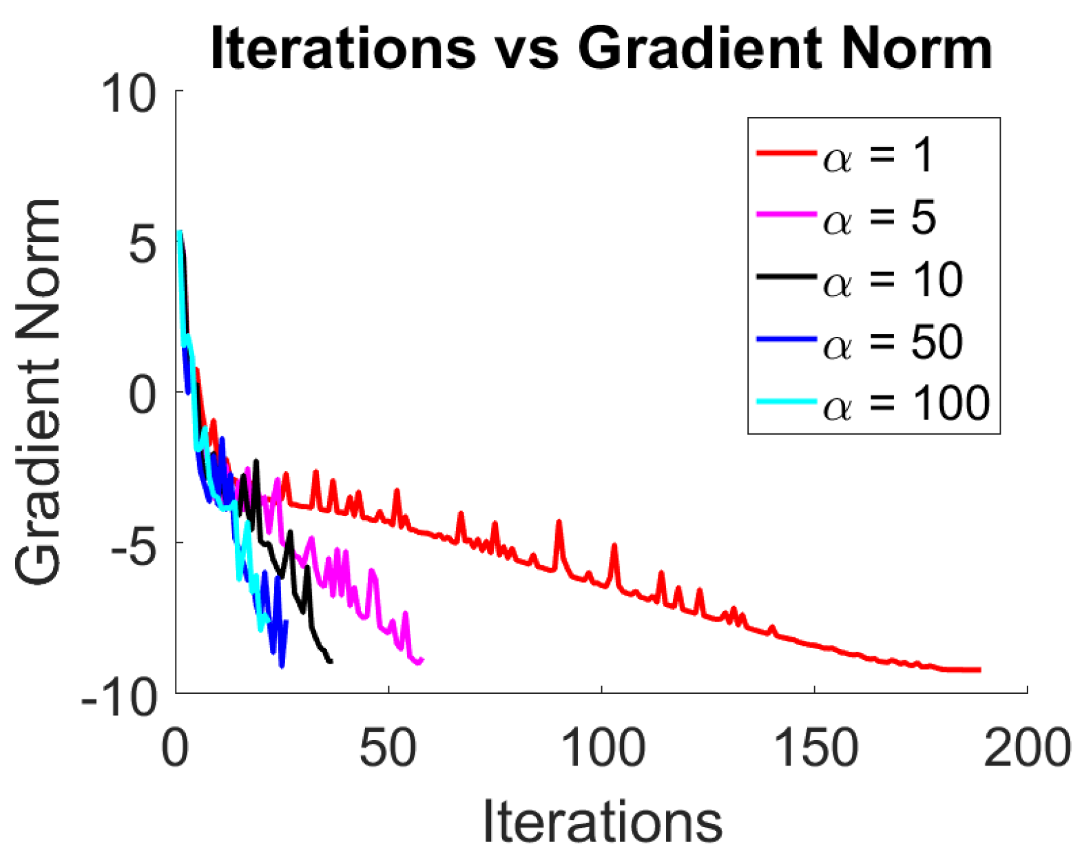
Firstly, we illustrate the numerical behavior of Algorithm 2 via varying the proximal parameter ${\alpha }_k$. Specifically, we conduct an experiment where we choose ${\alpha }_k=\alpha$ constant throughout the iterations process and solve an instance of Problem (30) with $(n,p)=(1000,100)$ for different values of $\alpha$. We randomly generate the matrix A as follows:

$$\mathtt{r}\mathtt{a}\mathtt{n}\mathtt{d}\mathtt{n}{(}^{\prime }see{d}^{\prime },1);B=\mathtt{r}\mathtt{a}\mathtt{n}\mathtt{d}\mathtt{n}(1000,100);A=0.5\ast (B^{\prime }+B),$$

using MATLAB’s commands, and we solve the problem for each $\alpha \in \{1,5,10,50,100\}$. In Figure 1, we present the convergence history of Algorithm 2 for all considered values of $\alpha$. In addition,

Table 1. Numerical performance of the PPASt scheme for different values of $\alpha$ in the solution of a randomly generated linear eigenvalue problem with $(n,p)=(1000,100)$.

$\mathit{\alpha }$	Nitr	Time	Grad	Feasi	Fval
1	189	11.145	9.99$\times {10}^{-5}$	3.10$\times {10}^{-15}$	3.657$\times {10}^3$
5	58	5.2831	9.70$\times {10}^{-5}$	3.89$\times {10}^{-15}$	3.657$\times {10}^3$
10	37	3.3362	9.76$\times {10}^{-5}$	3.77$\times {10}^{-15}$	3.657$\times {10}^3$
50	26	2.7402	4.93$\times {10}^{-5}$	3.64$\times {10}^{-15}$	3.657$\times {10}^3$
100	22	2.4424	4.39$\times {10}^{-5}$	3.84$\times {10}^{-15}$	3.657$\times {10}^3$

contains the numerical results associated with each value of $\alpha$. From Figure 1 and Table 1, we clearly see that Algorithm 2 requires a larger number of iterations to achieve the desired accuracy in the gradient norm for small values of $\alpha$.

Now, we consider the following experiment design: given $(n,p)$, we randomly generate dense matrices assembled as $A=0.5({\overline{A}}^{\top }+\overline{A})$, where $\overline{A}\in {\mathbb{R}}^{n \times n}$ is a matrix whose entries are sampled from a standard Gaussian distribution.

Table 2. Eigenvalues on randomly generated dense matrices for fixed $n=1000$.

p	1	50	100	300	500
	PPASt
Nitr	9.9	18.3	19.7	21.1	26.1
Time	0.04	0.89	1.75	9.51	21.64
Grad	3.79 $\times {10}^{-5}$	5.61$\times {10}^{-5}$	6.41 $\times {10}^{-5}$	6.31$\times {10}^{-5}$	7.51 $\times {10}^{-5}$
Feasi	1.67$\times {10}^{-16}$	2.13$\times {10}^{-15}$	3.53$\times {10}^{-15}$	7.89$\times {10}^{-15}$	1.19$\times {10}^{-14}$
Fval	44.4994	1.97$\times {10}^3$	3.64$\times {10}^3$	8.08$\times {10}^3$	9.49$\times {10}^3$
	OptStiefel
Nitr	141.3	273.4	293.3	295.1	336.7
Time	0.04	0.93	2.53	14.58	31.12
Grad	7.98$\times {10}^{-5}$	7.86$\times {10}^{-5}$	8.25$\times {10}^{-5}$	8.25$\times {10}^{-5}$	8.19$\times {10}^{-5}$
Feasi	8.88$\times {10}^{-17}$	2.59$\times {10}^{-14}$	3.05$\times {10}^{-14}$	1.65$\times {10}^{-14}$	1.59$\times {10}^{-14}$
Fval	44.4994	1.97$\times {10}^3$	3.64$\times {10}^3$	8.08$\times {10}^3$	9.49$\times {10}^3$
	RCG1a
Nitr	143.9	298.0	303.5	339.6	358.9
Time	0.06	1.59	4.39	30.64	78.21
Grad	8.48$\times {10}^{-5}$	8.34$\times {10}^{-5}$	8.02$\times {10}^{-5}$	8.78$\times {10}^{-5}$	8.56$\times {10}^{-5}$
Feasi	5.00$\times {10}^{-16}$	5.75$\times {10}^{-15}$	9.62$\times {10}^{-15}$	2.55$\times {10}^{-14}$	1.57$\times {10}^{-14}$
Fval	44.4994	1.97$\times {10}^3$	3.64$\times {10}^3$	8.08$\times {10}^3$	9.49$\times {10}^3$
	RCG1b
Nitr	137.2	288.7	296.1	309.9	360.8
Time	0.05	1.48	4.01	25.34	68.74
Grad	8.19$\times {10}^{-5}$	8.61$\times {10}^{-5}$	8.25$\times {10}^{-5}$	8.51$\times {10}^{-5}$	8.37$\times {10}^{-5}$
Feasi	3.55$\times {10}^{-16}$	6.22$\times {10}^{-15}$	1.01$\times {10}^{-14}$	2.55$\times {10}^{-14}$	1.57$\times {10}^{-14}$
Fval	44.4994	1.97$\times {10}^3$	3.64$\times {10}^3$	8.08$\times {10}^3$	9.49$\times {10}^3$
	RCG1b+ZH
Nitr	197.0	272.2	319.0	355.7	384.8
Time	0.06	1.25	3.99	27.24	67.52
Grad	7.84$\times {10}^{-5}$	8.10$\times {10}^{-5}$	8.53$\times {10}^{-5}$	8.60$\times {10}^{-5}$	8.29$\times {10}^{-5}$
Feasi	3.55$\times {10}^{-16}$	7.23$\times {10}^{-15}$	1.04$\times {10}^{-14}$	2.85$\times {10}^{-14}$	1.57$\times {10}^{-14}$
Fval	44.4994	1.97$\times {10}^3$	3.64$\times {10}^3$	8.08$\times {10}^3$	9.49$\times {10}^3$

contains the computational results associated with varying $p\in \{1,50,100,300,500\}$ but fixed $n=1000$. As shown in Table 2, all of the methods obtained estimates of a solution of Problem (30) with the required precision. Furthermore, we clearly observe that as p approaches n, our proposal converges more quickly, even in terms of computational time, than the rest of the methods.

5.2. Heterogeneous Quadratic Minimization

In this subsection, we consider the minimization of sums of heterogeneous quadratic functions over the Stiefel manifold; this problem is formulated as

$$\underset{X\in {\mathbb{R}}^{n \times p}}{min}\sum _{i=1}^{p}Tr\left[X_{\left[i\right]}^{\top }{A}_i{X}_{\left[i\right]}\right]\mathrm{s}.\mathrm{t}.X^{\top }X=I_p,$$

(31)

where $A_{i}s$ are n-by-n symmetric matrices and $X_{\left[i\right]}$ denotes the i-th column of X. For benchmarking, we consider two structures for the data matrices $A_{i}s$ obtained by using the following MATLAB commands:

• Structure I: $A_i=\mathtt{d}\mathtt{i}\mathtt{a}\mathtt{g}\left(\frac{(i-1)n+1}{p}:\frac{1}{p}:\frac{in}{p}\right)$, for all $i\in \{1,2,\dots ,p\}$.
• Structure II: $A_i=\mathtt{d}\mathtt{i}\mathtt{a}\mathtt{g}\left(\frac{(i-1)n+1}{p}:\frac{1}{p}:\frac{in}{p}\right)+B_i^{\top }+B_i$, for all $i\in \{1,2,\dots ,p\}$,

where $B_{i}s$ are random matrices generated by $B_i=0.1\mathtt{r}\mathtt{a}\mathtt{n}\mathtt{d}\mathtt{n}\left(n\right)$. This experiment design was taken from [13]. The numerical results concerning Structures I and II are contained in

Table 3. Numerical results of heterogeneous quadratic minimization considering Structure I.

Method	Nitr	Time	Grad	Feasi	Fval
	Structure I: $n=10000$, $p=10$
PPASt	76.7	3.25	8.14$\times {10}^{-5}$	8.17$\times {10}^{-16}$	4.50$\times {10}^4$
OptStiefel	1012.6	4.74	8.39$\times {10}^{-5}$	3.98$\times {10}^{-15}$	4.50$\times {10}^4$
RCG1a	1216.4	9.13	8.90$\times {10}^{-5}$	6.72$\times {10}^{-14}$	4.50$\times {10}^4$
RCG1b	1140.1	8.47	8.58$\times {10}^{-5}$	5.77$\times {10}^{-14}$	4.50$\times {10}^4$
RCG1b + ZH	1191.9	8.45	8.36$\times {10}^{-5}$	5.72$\times {10}^{-14}$	4.50$\times {10}^4$

and

Table 4. Numerical results of heterogeneous quadratics minimization considering Structure II.

Method	Nitr	Time	Grad	Feasi	Fval
	Structure II: $n=1000$, $p=5$
PPASt	57.6	16.09	8.21$\times {10}^{-5}$	7.66$\times {10}^{-16}$	1.99$\times {10}^3$
OptStiefel	592.1	14.27	8.18$\times {10}^{-5}$	2.86$\times {10}^{-15}$	1.99$\times {10}^3$
RCG1a	672.7	23.23	9.01$\times {10}^{-5}$	4.44$\times {10}^{-15}$	1.99$\times {10}^3$
RCG1b	643.6	21.77	8.50$\times {10}^{-5}$	4.05$\times {10}^{-15}$	1.99$\times {10}^3$
RCG1b + ZH	638.7	18.55	8.79$\times {10}^{-5}$	4.98$\times {10}^{-15}$	1.99$\times {10}^3$

, respectively. From Table 3, we see that the most efficient method both in terms of the number of iterations and in total computational time was our procedure. The second most efficient method was OptStiefel. However, the numerical performance of PPASt and OptStiefel is very similar.

On the other hand, the results related to Structure II show that OptStiefel is slightly superior to PPASt in terms of computational time. However our PPASt approach was much more efficient than the three Riemannian conjugate gradient methods and took fewer iterations to reach the desired tolerance than the rest of the methods. In addition, to illustrate the numerical efficiency of our proposal, we designed two randomized experiments where the initial points were built using the following MATLAB commands,

$$\mathtt{r}\mathtt{a}\mathtt{n}\mathtt{d}\mathtt{n}{(}^{\prime }see{d}^{\prime },1);[X_0,\sim ]=\mathtt{q}\mathtt{r}(\mathtt{r}\mathtt{a}\mathtt{n}\mathtt{d}\mathtt{n}(n,p),0),$$

and generated the heterogeneous quadratic minimization problems according to Structures I and II described above. In Figure 2 and Figure 3, we show the convergence history in terms of iterations and time (in seconds) of all the methods for these specific experiments. From these figures, we clearly see that our proximal point method converges faster (in terms of iterations) to a local minimizer than the rest of the methods, while in terms of computational time, the proposal achieves competitive results with respect to the other methods. Particularly, PPASt is the most efficient method for problems with Structure I.

5.3. The Joint Diagonalization Problem

Now, we evaluate the performance of our method on non-quadratic objective functions. Particularly, we consider the joint diagonalization problem [39], mathematically formulated as

$$\underset{X\in {\mathbb{R}}^{n \times p}}{max}\sum _{i=1}^N{\parallel Diag\left(X^{\top }{A}_{i}X\right)\parallel }_F^2\mathrm{s}.\mathrm{t}.X^{\top }X=I_p,$$

(32)

where the data $A_i$s are n-by-n symmetric matrices and $Diag\left(M\right)$ is the diagonal matrix obtained from M by replacing the non-diagonal elements of M with zero. In order to test all the algorithms, we randomly generate the matrices $A_i$s as follows

$$A_i=\mathtt{d}\mathtt{i}\mathtt{a}\mathtt{g}(\sqrt{n+1},\sqrt{n+2},\dots \sqrt{2n})+B_i+B_i^{\top },$$

where $B_i\in {\mathbb{R}}^{n \times n}$ is a random matrix whose entries are generated independently from a Gaussian distribution, and, given a vector $v\in {\mathbb{R}}^n$, $\mathtt{d}\mathtt{i}\mathtt{a}\mathtt{g}\left(v\right)$ denotes the diagonal matrix of size n-by-n whose i-th diagonal entry is exactly the i-th element of the vector v. This experiment was taken from [13]. We include in the numerical comparisons the Riemannian proximal gradient method (ManPG) developed in [7]. For this experiment, we generate ten independent instances for different values of n and p and report the mean values of Time, Nitr, Grad, Feasi, and Fval for each method. Additionally, we use $N=10000$ as the maximum number of iterations allowed for all the algorithms and we use $ϵ=1 \times {10}^{-5}$ as the tolerance for the termination rule associated with the gradient norm. The numerical results associated with this numerical test are presented in

Table 5. Numerical results on the joint diagonalization problem.

Method	Nitr	Time	Grad	Feasi	Fval
	$(n,p,N)=(500,3,3)$
OptStiefel	444.7	1.25	8.56$\times {10}^{-6}$	3.37$\times {10}^{-16}$	−3.59$\times {10}^4$
ManPG	9904.8	54.86	1.54$\times {10}^{-4}$	1.24$\times {10}^{-15}$	−3.59$\times {10}^4$
PPASt	27.6	1.51	6.10$\times {10}^{-6}$	3.67$\times {10}^{-16}$	−3.59$\times {10}^4$
RCG1a	547.7	2.41	7.87$\times {10}^{-6}$	2.49$\times {10}^{-15}$	−3.59$\times {10}^4$
RCG1b	570.7	2.24	7.97$\times {10}^{-6}$	2.52$\times {10}^{-15}$	−3.59$\times {10}^4$
RCG1b + ZH	605.3	1.94	7.39$\times {10}^{-6}$	2.03$\times {10}^{-15}$	−3.59$\times {10}^4$
	$(n,p,N)=(500,3,5)$
OptStiefel	634.2	4.11	8.59$\times {10}^{-6}$	9.25$\times {10}^{-16}$	−4.60$\times {10}^4$
ManPG	11232.0	97.74	2.25$\times {10}^{-4}$	1.04$\times {10}^{-15}$	−4.60$\times {10}^4$
PPASt	32.1	3.40	7.48$\times {10}^{-6}$	2.85$\times {10}^{-16}$	−4.60$\times {10}^4$
RCG1a	654.6	4.82	8.44$\times {10}^{-6}$	2.41$\times {10}^{-15}$	−4.60$\times {10}^4$
RCG1b	653.7	4.76	7.85$\times {10}^{-6}$	2.61$\times {10}^{-15}$	−4.60$\times {10}^4$
RCG1b + ZH	770.0	4.44	7.91$\times {10}^{-6}$	2.92$\times {10}^{-15}$	−4.60$\times {10}^4$
	$(n,p,N)=(1000,3,3)$
OptStiefel	1702.5	25.36	8.90$\times {10}^{-6}$	3.84$\times {10}^{-16}$	−7.28$\times {10}^4$
ManPG	19801.0	426.69	3.54$\times {10}^{-2}$	8.66$\times {10}^{-16}$	−7.28$\times {10}^4$
PPASt	57.2	13.71	6.91$\times {10}^{-6}$	3.22$\times {10}^{-16}$	−7.28$\times {10}^4$
RCG1a	1277.1	22.03	8.28$\times {10}^{-6}$	2.02$\times {10}^{-15}$	−7.28$\times {10}^4$
RCG1b	1207.2	20.75	8.26$\times {10}^{-6}$	2.47$\times {10}^{-15}$	−7.28$\times {10}^4$
RCG1b + ZH	1216.6	17.01	8.75$\times {10}^{-6}$	2.82$\times {10}^{-15}$	−7.28$\times {10}^4$
	$(n,p,N)=(1000,3,5)$
OptStiefel	2194.3	50.45	3.40$\times {10}^{-6}$	3.34$\times {10}^{-16}$	−9.26$\times {10}^4$
ManPG	15401.0	505.59	3.10$\times {10}^{-3}$	8.01$\times {10}^{-16}$	−9.26$\times {10}^4$
PPASt	46.8	18.59	6.68$\times {10}^{-6}$	3.52$\times {10}^{-16}$	−9.26$\times {10}^4$
RCG1a	1045.3	30.71	7.71$\times {10}^{-6}$	2.14$\times {10}^{-15}$	−9.26$\times {10}^4$
RCG1b	1019.9	30.01	8.58$\times {10}^{-6}$	1.83$\times {10}^{-15}$	−9.26$\times {10}^4$
RCG1b + ZH	996.0	22.95	8.22$\times {10}^{-6}$	1.64$\times {10}^{-15}$	−9.26$\times {10}^4$

.

From Table 5, we see that the ManPG method obtains very poor performance, which is possibly due to the step-size used to initialize the backtracking process being set to ${\alpha }_k^{\mathrm{ini}}=1$ in each iteration, which can lead to the method carrying out many re-orthogonalizations and function evaluations per iteration. Furthermore, we notice that our proposal was the most efficient both in terms of total computational time and in the number of iterations. In fact, in terms of CPU time, the OptStiefel method is better than PPASt only for instances with $(n,p,N)=(500,3,3)$, while for the rest of the instances, our PPASt outperforms the other methods.

6. Conclusions

In this article, we introduced a new, feasible method, free of exponential mapping, for solving smooth optimization problems on the Stiefel manifold. In particular, the proposal is an exact proximal point algorithm constructed with the standard distance of the matrix space ${\mathbb{R}}^{n \times p}$ that exploits the geometric properties of the Stiefel manifold. The proposed algorithm constructs a sequence $\left\{X_k\right\}\subset St(n,p)$ through an iterative process that successively applies a simple proximal operator to the initial point $X_0$. The global convergence of the proposed approach was established. In addition, we demonstrated that every accumulation point of the sequence generated by the algorithms is a stationary point without imposing any restrictive hypotheses on the objective function. Since the proposed algorithm is a special case of PALM [30], inertial extensions are already discussed in [32,40]. Our computational studies show that the developed method can be a good tool to solve trace maximization problems and heterogeneous quadratic minimization problems on the Stiefel manifold.

Similarly to the proofs presented in [30,40], we can try to establish convergence of the sequence $\left\{X_k\right\}$ to a critical point of $\mathcal{F}$ under the Kurdyka–Lojasiewicz property. These idea will remain as future work.