A Novel Neighborhood Granular Meanshift Clustering Algorithm

Abstract

The most popular algorithms used in unsupervised learning are clustering algorithms. Clustering algorithms are used to group samples into a number of classes or clusters based on the distances of the given sample features. Therefore, how to define the distance between samples is important for the clustering algorithm. Traditional clustering algorithms are generally based on the Mahalanobis distance and Minkowski distance, which have difficulty dealing with set-based data and uncertain nonlinear data. To solve this problem, we propose the granular vectors relative distance and granular vectors absolute distance based on the neighborhood granule operation. Further, the neighborhood granular meanshift clustering algorithm is also proposed. Finally, the effectiveness of neighborhood granular meanshift clustering is proved from two aspects of internal metrics (Accuracy and Fowlkes–Mallows Index) and external metric (Silhouette Coeffificient) on multiple datasets from UC Irvine Machine Learning Repository (UCI). We find that the granular meanshift clustering algorithm has a better clustering effect than the traditional clustering algorithms, such as Kmeans, Gaussian Mixture and so on.

1. Introduction

The American scientist Zadeh proposed the theory of fuzzy sets in 1965 [1]. The theory is an extension of classical set theory and describes uncertainty problems by using an affiliation function. The rough set theory proposed by Polish mathematician Pawlak [2] is likewise one of the widely adopted models for uncertain systems. In rough set theory, the equivalence class is regarded as an elementary granule. For real-world widely available real-type data, a discretization process is required, which is prone to loss of categorical information. For this purpose, Yao [3] proposed a neighborhood rough set model. In 1999, Lin, a Hong Kong scholar, proposed a novel data mining algorithm based on granular computing [4], which laid the foundation for the application of granular computing to various fields. Additionally, Yager [5] pointed out that the way humans think is also related to granularity. After this, the field of granular computing has attracted a large number of scholars, and considerable results have been achieved in all the given fields [6,7,8,9,10]. In 2008, Hu et al. proposed a neighborhood rough set-based attribute approximate reduction algorithm to enhance the effectiveness of the nearest neighbor algorithm [11]. Qian et al. proposed a model for learning decisions under different granularity patterns [12]. In order to improve the theory of rough grain calculation, Miao et al. [13] make a systematic study of the granular computing using the logic language L. In 2014, Qian [14] designed a parallelized attribute approximate subtraction algorithm to improve the efficiency of granular computing operations on attribute approximate subtraction problems. Chen [15,16] applied rough sets to the swarm intelligence algorithm, which not only further extended the application of granular computing, but also improved the effectiveness of the swarm intelligence algorithm. Further, a novel variant of rough granules based on the neighborhood system was also defined by Chen et al. [17]. With the development of granular computing theory, granular computing has gradually penetrated into various fields, such as image processing [18], clustering [19,20,21], classification [22,23,24], neural networks [25,26,27], and human–robot interaction [28].

Clustering is a very common data processing method in unsupervised learning. It is a method of dividing data into corresponding clusters according to certain attributes of the data. The similarity of data in the same cluster should be as large as possible, while the similarity between clusters should be as small as possible for clustering. It plays an important role in data mining, pattern recognition, and other fields. Meanshift algorithm is one of the research hotspots in the clustering algorithm. The general algorithm can only solve the clustering problem of data sets whose data structure is similar to spherical or clique, while ineffectively clustering edge points and outliers. However, the Meanshift clustering algorithm can cluster correctly in the data set of the data structure type with arbitrary shape distribution, and it has strong anti-noise. The Meanshift algorithm is a gradient-based non-parametric density estimation algorithm. The maximum value of the probability density distribution is in the upward direction of the probability distribution of the gradient. After effective statistical iterative calculations, the data points are finally clustered into the area with the largest local probability density to form different cluster classes. In recent years, it has been widely used in target tracking, image segmentation, and other fields. The Meanshift algorithm was proposed by Fukunaga and Hostetler in 1975, and its basic idea is to use gradient climbing of the probability density to find a local optimum [29]. Cheng [30] defines a kind of kernel function for the characteristics that the closer the data are to the cluster center, the better the cluster center statistics are. Comaniciu [29,31] introduced the bandwidth parameter for analyzing complex multimodal eigenspaces and depicting arbitrarily shaped clusters in them. In [32], an Epanechnikov-meanshifit clustering algorithm based on the “optimal” Epanechnikov kernel density estimator was designed to locate the centroids of the data clusters. However, the traditional Meanshift algorithm uses the Mahalanobis distance or Minkowski distance for the metric between data points. That makes the Meanshift algorithm ineffective in set data and uncertain nonlinear data. In recent years, for the clustering process of uncertain nonlinear datasets, many scholars have focused more on the dimension of nonlinear datasets. Lai [33] proposed two novel methods, termed kernel competitive learning (KCL) and graph-based multi-prototype competitive learning (GMPCL), to address the nonlinearly separable problem suffered by the classical competitive learning clustering algorithms. Chen [34] proposed a new nonlinear clustering method based on crowd movement and selection (CCMS) to focus on the data points themselves and the data distribution of their neighborhood. Qin [35] proposed a novel data model termed Hybrid K-Nearest-Neighbor (HKNN) graph, which combines the advantages of mutual k-nearest-neighbor graph and k-nearest-neighbor graph, to represent the nonlinear data sets. For the set-based data and uncertain nonlinear data, in this paper the neighborhood granulation method is defined in terms of the neighborhood system, starting from the distance metrics between data. Further, two new distance metrics methods (granular vector distance) between data are proposed, using the metric and operation relations in the neighborhood system. Finally, a new neighborhood granular meanshift clustering algorithm is constructed to provide an effective clustering method for uncertain nonlinear data sets.

This paper is organized into several sections. In the first section, we introduce the development of granular computation and clustering algorithms in recent years. Then, we introduce neighborhood granulation methods and granular vectors. In Section 3, we propose the granular meanshift algorithm based on two granular vectors distance metrics. After that, the experimental analysis of the granular meanshift algorithm is given in Section 4. Finally, we conclude the whole paper in Section 5.

2. Granulation

Chen et al. [17] granulated the sample in the neighborhood system with the single atomic feature.

2.1. Neighborhood Granulation

Definition 1.

Let the clustering system be $CS=(S,F)$. For the sample $\forall x,y\in S$, and single-atom characteristics $\forall a\in F$. Define the distance function of the samples x, y on the single atomic feature a as:

$$D(x,y)=\left|u\right(x,a)-u(y,a\left)\right|,$$

(1)

where $u(x,a)$ denotes the value of sample x on feature a.

Definition 2.

Let the clustering system be $CS=(S,F)$, and the neighborhood granular parameter be δ. For a sample $\forall x\in S$, a single atomic feature $\forall a\in F$, the δ neighborhood granules of x on a is defined as:

$$g_a{\left(x\right)}_{\delta }=\left\{y\right|x,y\in S,D_a(x,y)\le \delta \}.$$

(2)

$r_j$ is the distance between sample x and sample $x_j$ on feature c. It is easy to know from Definition 1 that $r_j=s_c\left(x,x_j\right)\in [0,1]$. We define $g_c\left(x\right)$ as the granule and $g_c{\left(x\right)}_j$ as the $jth$ granule kernels of the granule $g_c\left(x\right)$, and the granule consists of the granule kernels.

Definition 3.

Let the clustering system be $CS=(S,F)$ and the neighborhood granular parameter be δ. For a sample $\forall x\in S$, a single atomic feature $\forall a\in F$, the size of the neighborhood granules $g_a{\left(x\right)}_{\delta }$ is defined as:

$$Size\left(g_a{\left(x\right)}_{\delta }\right)=\left|g_a{\left(x\right)}_{\delta }\right|.$$

(3)

Definition 4.

Let the clustering system be $CS=(S,F)$ and the neighborhood granular parameter be δ. For a sample $\forall x\in S$, the feature subset $\forall P\subseteq F$, let $P=\{a_1,a_2,\dots ,a_m\}$, then the δ-neighborhood granular vector of x on the characteristic subset P is defined as:

$$V_P{\left(x\right)}_{\delta }=(g_{a_1}{\left(x\right)}_{\delta },g_{a_2}{\left(x\right)}_{\delta },\dots ,g_{a_m}{\left(x\right)}_{\delta }).$$

(4)

$g_a{\left(x\right)}_{\delta }$ is a $\delta$-neighborhood granule of sample x on characteristic a, in the form of a set. It is called an element of the granular vector, referred to as the granular element. $V_P{\left(x\right)}_{\delta }$ is a granular vector, consisting of granular elements. Thus, the elements of a granular vector are sets, unlike a traditional vector, whose elements are real numbers. When the elements of a granular vector are all 0, it is called a null granular vector and is denoted as $V_{null}$. When the elements of the granular vector are all 1, it is called a full granular vector, denoted as $V_{full}$.

Definition 5.

For a sample $\forall x\in S$, the feature subset $\forall P\subseteq F$, let $P=\{a_1,a_2,\dots ,a_m\}$. the size of the neighborhood granular vector $V_P{\left(x\right)}_{\delta }$ of x on the characteristic subset P is defined as:

$$|V_P{\left(x\right)}_{\delta }|=\sqrt{\sum _{i=1}^m|g_{a_i}{\left(x\right)}_{\delta }{|}^2}.$$

(5)

The size of the granular vector $V_P{\left(x\right)}_{\delta }$ is also called the norm of the granular vector.

2.2. Granular Vector Operations

In this subsection, we give the granular vector operations.

Definition 6.

There is a clustering system $CS=(S,F)$. $\forall x\in S$. There exists a δ-neighborhood of granular vectors $V_F{\left(x\right)}_{\delta }$ on F. The set of all granular vectors on F is called the set of granular vectors and is defined as:

$$Group{V}_F{\left(x\right)}_{\delta }=\left\{V_F{\left(x\right)}_{\delta }\right|\forall x\in S\}.$$

(6)

Definition 7.

There is a clustering system $CS=(S,F)$, where the feature set is $F=(a_1,a_2,\dots ,a_m)$. For $\forall x,y\in S$, there exist 2 δ-neighborhood granular vectors on F as $V_F{\left(x\right)}_{\delta }=(g_{a_1}{\left(x\right)}_{\delta },\dots ,g_{a_m}{\left(x\right)}_{\delta })$, $V_F{\left(y\right)}_{\delta }=(g_{a_1}{\left(y\right)}_{\delta },\dots ,g_{a_m}{\left(y\right)}_{\delta })$. The intersection, concatenation, addition, subtraction and dissimilarity operations of the 2 granular vectors are defined as:

$$V_F{\left(x\right)}_{\delta }\wedge V_F{\left(y\right)}_{\delta }=(g_{a_1}{\left(x\right)}_{\delta }\wedge g_{a_1}{\left(y\right)}_{\delta },g_{a_2}{\left(x\right)}_{\delta }\wedge g_{a_2}{\left(y\right)}_{\delta },\dots ,g_{a_m}{\left(x\right)}_{\delta }\wedge g_{a_m}{\left(y\right)}_{\delta }),$$

(7)

$$V_F{\left(x\right)}_{\delta }\vee V_F{\left(y\right)}_{\delta }=(g_{a_1}{\left(x\right)}_{\delta }\vee g_{a_1}{\left(y\right)}_{\delta },g_{a_2}{\left(x\right)}_{\delta }\vee g_{a_2}{\left(y\right)}_{\delta },\dots ,g_{a_m}{\left(x\right)}_{\delta }\vee g_{a_m}{\left(y\right)}_{\delta }),$$

(8)

$$V_F{\left(x\right)}_{\delta }+V_F{\left(y\right)}_{\delta }=(g_{a_1}{\left(x\right)}_{\delta }+g_{a_1}{\left(y\right)}_{\delta },g_{a_2}{\left(x\right)}_{\delta }+g_{a_2}{\left(y\right)}_{\delta },\dots ,g_{a_m}{\left(x\right)}_{\delta }+g_{a_m}{\left(y\right)}_{\delta }),$$

(9)

$$V_F{\left(x\right)}_{\delta }-V_F{\left(y\right)}_{\delta }=(g_{a_1}{\left(x\right)}_{\delta }-g_{a_1}{\left(y\right)}_{\delta },g_{a_2}{\left(x\right)}_{\delta }-g_{a_2}{\left(y\right)}_{\delta },\dots ,g_{a_m}{\left(x\right)}_{\delta }-g_{a_m}{\left(y\right)}_{\delta }),$$

(10)

$$V_F{\left(x\right)}_{\delta }\oplus V_F{\left(y\right)}_{\delta }=(g_{a_1}{\left(x\right)}_{\delta }\oplus g_{a_1}{\left(y\right)}_{\delta },g_{a_2}{\left(x\right)}_{\delta }\oplus g_{a_2}{\left(y\right)}_{\delta },\dots ,g_{a_m}{\left(x\right)}_{\delta }\oplus g_{a_m}{\left(y\right)}_{\delta }).$$

(11)

3. Granular Meanshift Based on Neighborhood Systems

The neighborhood granular meanshift algorithm is an unsupervised clustering algorithm. Unlike the Meanshift algorithm, the granular meanshift algorithm uses the granular vector as the minimum unit of operation. Because the granular vector contains global information, which means the neighborhood granular meanshift algorithm has better clustering performance compared to the Meanshift algorithm.

3.1. Granular Vector Metric

Defining the distance metric of the granular vectors is the basis for constructing a clustering algorithm based on granular vectors. By defining the granular vector operations, we can next define the granular vectors relative distance and the granular vectors absolute distance.

Definition 8.

For $\forall x,y\in S$, there exist 2 δ-neighborhood granular vectors on F as $V_F{\left(x\right)}_{\delta }=(g_{a_1}{\left(x\right)}_{\delta },g_{a_2}{\left(x\right)}_{\delta },\dots ,g_{a_m}{\left(x\right)}_{\delta })$, $V_F{\left(y\right)}_{\delta }=(g_{a_1}{\left(y\right)}_{\delta },g_{a_2}{\left(y\right)}_{\delta },\dots ,g_{a_m}{\left(y\right)}_{\delta })$, then the relative distance between $V_F{\left(x\right)}_{\delta }$ and $V_F{\left(y\right)}_{\delta }$ is defined as:

$$\begin{array}{cc}\hfill d_1(V_F{\left(x\right)}_{\delta },V_F{\left(y\right)}_{\delta })& =\frac{1}{\left|F\right|\times \left|S\right|}\frac{|g_{a_i}{\left(x\right)}_{\delta }\oplus g_{a_i}{\left(y\right)}_{\delta }|}{|g_{a_i}{\left(x\right)}_{\delta }\vee g_{a_i}{\left(y\right)}_{\delta }|}\hfill \\ \hfill & =\frac{1}{\left|F\right|}\left(\frac{|g_{a_1}{\left(x\right)}_{\delta }\oplus g_{a_1}{\left(y\right)}_{\delta }|}{|g_{a_1}{\left(x\right)}_{\delta }\vee g_{a_1}{\left(y\right)}_{\delta }|}+\dots +\frac{|g_{a_m}{\left(x\right)}_{\delta }\oplus g_{a_m}{\left(y\right)}_{\delta }|}{|g_{a_m}{\left(x\right)}_{\delta }\vee g_{a_m}{\left(y\right)}_{\delta }|}\right).\hfill \end{array}$$

(12)

Definition 9.

For $\forall x,y\in S$, there exist 2 δ-neighborhood granular vectors on F as $V_F{\left(x\right)}_{\delta }=(g_{a_1}{\left(x\right)}_{\delta },g_{a_2}{\left(x\right)}_{\delta },\dots ,g_{a_m}{\left(x\right)}_{\delta })$, $V_F{\left(y\right)}_{\delta }=(g_{a_1}{\left(y\right)}_{\delta },g_{a_2}{\left(y\right)}_{\delta },\dots ,g_{a_m}{\left(y\right)}_{\delta })$, then the absolute distance between $V_F{\left(x\right)}_{\delta }$ and $V_F{\left(y\right)}_{\delta }$ is defined as:

$$\begin{array}{cc}\hfill d_2(V_F{\left(x\right)}_{\delta },V_F{\left(y\right)}_{\delta })& =\frac{1}{\left|F\right|\times \left|S\right|}\sum _{i=1}^m|g_{a_i}{\left(x\right)}_{\delta }\oplus g_{a_i}{\left(y\right)}_{\delta }|\hfill \\ \hfill & =\frac{1}{\left|F\right|\times \left|S\right|}\left(\right|g_{a_i}{\left(x\right)}_{\delta }\oplus g_{a_i}{\left(y\right)}_{\delta }|+\dots +|g_{a_m}{\left(x\right)}_{\delta }\oplus g_{a_m}{\left(y\right)}_{\delta }\left|\right).\hfill \end{array}$$

(13)

It is easy to see from Definitions 8 and 9 that $0\le d_1(V_F{\left(x\right)}_{\delta },{\left(y\right)}_{\delta })\le 1$, and $0\le d_2(V_F{\left(x\right)}_{\delta },V_F{\left(y\right)}_{\delta })\le 1$. We give the proof below.

Proof 1.

From $|g_{a_i}{\left(x\right)}_{\delta }\oplus g_{a_i}{\left(y\right)}_{\delta }| = |g_{a_i}{\left(x\right)}_{\delta }\vee g_{a_i}{\left(y\right)}_{\delta }-g_{a_i}{\left(x\right)}_{\delta }\wedge g_{a_i}{\left(y\right)}_{\delta }|$, it follows that $|g_{a_i}{\left(x\right)}_{\delta }\oplus g_{a_i}{\left(y\right)}_{\delta }| = |g_{a_i}{\left(x\right)}_{\delta }\vee g_{a_i}{\left(y\right)}_{\delta }-g_{a_i}{\left(x\right)}_{\delta }\wedge g_{a_i}{\left(y\right)}_{\delta }|$, then $0\le \frac{|g_{a_i}{\left(x\right)}_{\delta }\oplus g_{a_i}{\left(y\right)}_{\delta }|}{|g_{a_i}{\left(x\right)}_{\delta }\vee g_{a_i}{\left(y\right)}_{\delta }|}\le 1$.

Given that $F=(a_1,a_2,\dots ,a_m)$, we know that $\left|F\right|=m$.

Thus, $0\le {\sum }_{i=1}^m\frac{|g_{a_i}{\left(x\right)}_{\delta }\oplus g_{a_i}{\left(y\right)}_{\delta }|}{|g_{a_i}{\left(x\right)}_{\delta }\vee g_{a_i}{\left(y\right)}_{\delta }|}\le \left|F\right|$, which makes $0\le \frac{1}{\left|F\right|}{\sum }_{i=1}^m\frac{|g_{a_i}{\left(x\right)}_{\delta }\oplus g_{a_i}{\left(y\right)}_{\delta }|}{|g_{a_i}{\left(x\right)}_{\delta }\vee g_{a_i}{\left(y\right)}_{\delta }|}\le 1$.

By Definition 8, it holds that $0\le d_1(V_F{\left(x\right)}_{\delta },{\left(y\right)}_{\delta })\le 1$.    □

Proof 2.

From $|g_{a_i}{\left(x\right)}_{\delta }\oplus g_{a_i}{\left(y\right)}_{\delta }|=|g_{a_i}{\left(x\right)}_{\delta }\vee g_{a_i}{\left(y\right)}_{\delta }-g_{a_i}{\left(x\right)}_{\delta }\wedge g_{a_i}{\left(y\right)}_{\delta }|$, it is clear that $0\le |g_{a_i}{\left(x\right)}_{\delta }\oplus g_{a_i}{\left(y\right)}_{\delta }|\le |S|$.

By $F=(a_1,a_2,\dots ,a_m)$, we know that $\left|F\right|=m$, then $0\le {\sum }_{i=1}^m|g_{a_i}{\left(x\right)}_{\delta }\oplus g_{a_i}{\left(y\right)}_{\delta }|\le \left|F\right|\times \left|S\right|$.

Since $d_2(V_F{\left(x\right)}_{\delta },V_F{\left(y\right)}_{\delta })=\frac{1}{\left|F\right|\times \left|S\right|}{\sum }_{i=1}^m|g_{a_i}{\left(x\right)}_{\delta }\oplus g_{a_i}{\left(y\right)}_{\delta }|$, the $0\le d_2(V_F{\left(x\right)}_{\delta },V_F{\left(y\right)}_{\delta })\le 1$ holds.    □

3.2. Neighborhood Granular Meanshift Clustering Theory

In the following, we give the basic principles of the granular meanshift clustering algorithm. Granular meanshift clustering is an iterative algorithm. First, a granular vector is randomly selected as the barycenter granular vector. After that, we calculate the average of all granular vectors with distance less than h from the barycenter granular vector. This average is then added to the barycenter granular vector to form the new barycenter granular vector. By iterating continuously, when the change of barycenter granular vector is less than a threshold, this iteration process is ended, and all the granular vectors in this iteration are added to the cluster c. After all the granular vectors have been visited, we start merging the subclusters of the cluster C. If the distance between two clusters’ barycenter granular vectors is less than a threshold, the two sub-clusters are merged into one sub-cluster.

Neighborhood granular meanshift is an algorithm based on the barycenter granular vector, which we define as the average of the sum of all granular vectors in the same cluster. In the following, we give the formula for the barycenter granular vector.

Definition 10.

Let the clustering system be $CS=\left(S,F\right)$, where the feature set is $F=(a_1,a_2,\dots ,$$a_m)$. For $x_1,x_2,\dots {,x}_n\subseteq S$, there are n neighborhood granular vectors as $\{V_F{\left(x_1\right)}_{\delta },V_F{\left(x_2\right)}_{\delta },\dots ,$$V_F{\left(x_n\right)}_{\delta }\}$. Its barycenter granular vector is given by:

$${GV}_{FC}\left(x\right)=\frac{{\sum }_{i=1}^n{V}_F{\left(x_i\right)}_{\delta }}{n}.$$

(14)

The general Meanshift algorithm can use the RBF kernel function to enhance the clustering effect, and similarly we define the granular RBF function on the granular vector space.

Definition 11.

Let the clustering system be $CS=\left(S,F\right)$, where the feature set is $F=(a_1,a_2,\dots ,$$a_m)$. For $\forall x,y\in S$, there exist 2 δ neighborhood granular vectors as $V_F{\left(x\right)}_{\delta }=(g_{a_1}{\left(x\right)}_{\delta },g_{a_2}{\left(x\right)}_{\delta },$$\dots ,g_{a_m}{\left(x\right)}_{\delta })$, $V_F{\left(x\right)}_{\delta }=(g_{a_1}{\left(x\right)}_{\delta },g_{a_2}{\left(x\right)}_{\delta },\dots ,g_{a_m}{\left(x\right)}_{\delta })$. The granular RBF function of the distance is

$$k(V_F{\left(x\right)}_{\delta },V_F{\left(y\right)}_{\delta })=\frac{1}{h\sqrt{2\pi }}{e}^{-\frac{d^2(V_F{\left(x\right)}_{\delta },V_F{\left(y\right)}_{\delta })}{2h^2}}.$$

(15)

3.3. Neighborhood Granular Meanshift Clustering Algorithm Implementation

After defining the barycenter granular vector and the granular RBF function, we propose the neighborhood granular meanshift clustering algorithm based on the granular vectors absolute distance and granular vectors relative distance in Algorithm 1.

Algorithm 1 Granular meanshift clustering algorithm

Input: The data set is $CS=(S,F)$, where the sample set is $S=x_1,x_2,\dots ,x_n$ the set of attributes is $F=a_1,a_2,\dots ,a_m$; the neighborhood parameter $\delta$, the maximum number of iterations N; the bandwidth parameter h, granular vectors distance threshold $d_{thre}$. Output: Cluster division $C=(C_1,C_2,\dots ,C_K)$. 1: The sample set U is granularized as $GT=\{V_F\left(x_1\right),V_F\left(x_2\right),\dots ,V_F\left(x_n\right)\}$ 2: while do 3:    Select an unlabeled neighborhood granular vector from the $GT$ as the barycenter, denoted as ${GV}_{FC}\left(x_j\right)(j=1,2,\dots ,n)$. 4:    for i to N do 5:      With $G_{FC}\left(x_j\right)$ as the center and h as the radius, the set is obtained $M=S\left(x_j\right)\cup x_j:S\left(x_j\right)=x_i:d_{ij}(G_{FC}\left(x_j\right),G_F\left(x_i\right))\le h^2(i=1,2,\dots ,n)$. The set M belongs to the cluster $C_j$, update the sample probability $p_{C_j}\left(x\right)=p_{C_j}\left(x\right)+1;x\in M$ within cluster $C_j$. 6:      Calculate the granular vectors distance $d_{ij}$ of the granular barycenter vector ${GV}_{FC}\left(x_j\right)$ to each neighboring granular vector $V_F\left(x_i\right)$ of the elements in the set M. For $x_i\in M$, use all $d_{ij}$ for recomputing the new granular barycenter vector ${GV}_{F{C}_{n}ew}\left(x_j\right)={\left[{\sum }_{x_i\in M}k\left(d_{ij}\right)\right]}^{-1}•{\sum }_{x_i\in M}k\left(d_{ij}\right)•V_F\left(x_i\right)$. 7:      If the granular barycenter vector $G_{FC}\left(x_j\right)$ is no longer changing, go to step (9) 8:    end for 9:    If all points in GT are visited, go to step (11). 10: end while 11: For ${GV}_{FC}\left(x_j\right)$ with ${GV}_{FC}\left(x_i\right)$, if it satisfies $d_{ij}({GV}_{FC}\left(x_i\right),{GV}_{FC}\left(x_j\right))\le d_{thre}$. Merge the cluster classes $C_j \mathrm{and} C_i$, and update $p_{C_j}\left(x\right)$ and $p_{C_i}\left(x\right)$. 12: Output clusters $C=(C_1,C_2,\dots ,C_K)$.

4. Experimental Analysis

All the experimental results in this paper are conducted by Python 3.8 under the Microsoft Windows 10 system based on the Intel Core i5-12600K high-performance processor hardware platform. Five UCI public data sets of Cintraceptive-Method-Choice (CMC), Iris, Heart Disease, Wine, and Pima-Indians-diabetes (Pim) are used to verify the effectiveness of the proposed algorithm, including linearly separable and non-linearly separable data sets, as shown in

Table 1. Descriptions of datasets.

Datasets	Samples	Features	Categories
CMC	1473	9	3
Iris	150	4	3
Heart Disease	303	13	2
Wine	178	13	3
Pim	768	8	2

. Since the feature amplitude of each data is different, the data is normalized by the maximum and minimum values, and the value range of each feature is converted to [0, 1].

After data preprocessing, the data is granulated according to the neighborhood parameters to generate granular vectors. Since there are relative distance and absolute distance formulas for estimating the distance between granular vectors, this experiment proposes a granular meanshift clustering algorithm based on granular vectors relative distance and granular vectors relative distance. At the same time, to verify the performance of the algorithm, it will be compared with Meanshift and the other 5 classic clustering algorithms.

In this experiment, the performance of granular meanshift clustering algorithm is optimized by adjusting the Neighborhood Granular Parameter (NGP), then three clustering performance evaluation indicators: Accuracy, Silhouette Coefficient (SC), and Fowlkes–Mallows Index (FMI) are used for clustering performance comparison. Accuracy is defined as follows:

$$Accuracy=\frac{{\sum }_{i=1}^N\phi (s_i,map\left(r_i\right))}{N}.$$

(16)

Among them, $r_i$ is the label after clustering, $s_i$ is the real label, and N is the total number of data samples. $\phi$ represents the indicator function, as follows:

$$\phi (x,y)=\left\{\begin{array}{cc}1,\hfill & x=y\hfill \\ 0,\hfill & x\ne y\hfill \end{array}\right..$$

(17)

To express SC, the silhouette coefficient $s\left(i\right)$ of a single sample is:

$$s\left(i\right)=\frac{b\left(i\right)-a\left(i\right)}{max\left\{a\right(i),b(i\left)\right\}}.$$

(18)

Among them, $a\left(i\right):i\in A,a\left(i\right)=averag{e}_{j\in A,j\ne i}\left(dist(i,j)\right)$; $b\left(i\right):i\in A,C\ne A,dist(i,C)=averag{e}_{j\in C}\left(dist(i,j)\right)$; $b\left(i\right)={min}_{C\ne A}dist(i,C)$. Both A and C are clusters of sample i. Then, the SC is defined as follows:

$$s\left(i\right)=\frac{b\left(i\right)-a\left(i\right)}{max\left\{a\right(i),b(i\left)\right\}}.$$

(19)

The FMI is defined as follows:

$$FMI=\frac{TP}{\sqrt{(TP+FP)(TP+FN)}}.$$

(20)

TP is the number of True Positives; FP is the number of False Positives; and FN is the number of False Negatives.

Accuracy directly represents the performance of the clustering algorithm, the value range is [0, 1], and the larger the value, the better the clustering effect. SC represents the similarity of samples within a cluster and the difference between clusters, and the value range is [−1, 1]. The smaller the difference within a cluster and the larger the difference between clusters, the better the clustering effect. The FMI indicator is the geometric mean of precision and recall and is used to determine the similarity between two data sets. The larger the FMI value, the higher the similarity between the real data set and the predicted data set, and its value range is [0, 1].

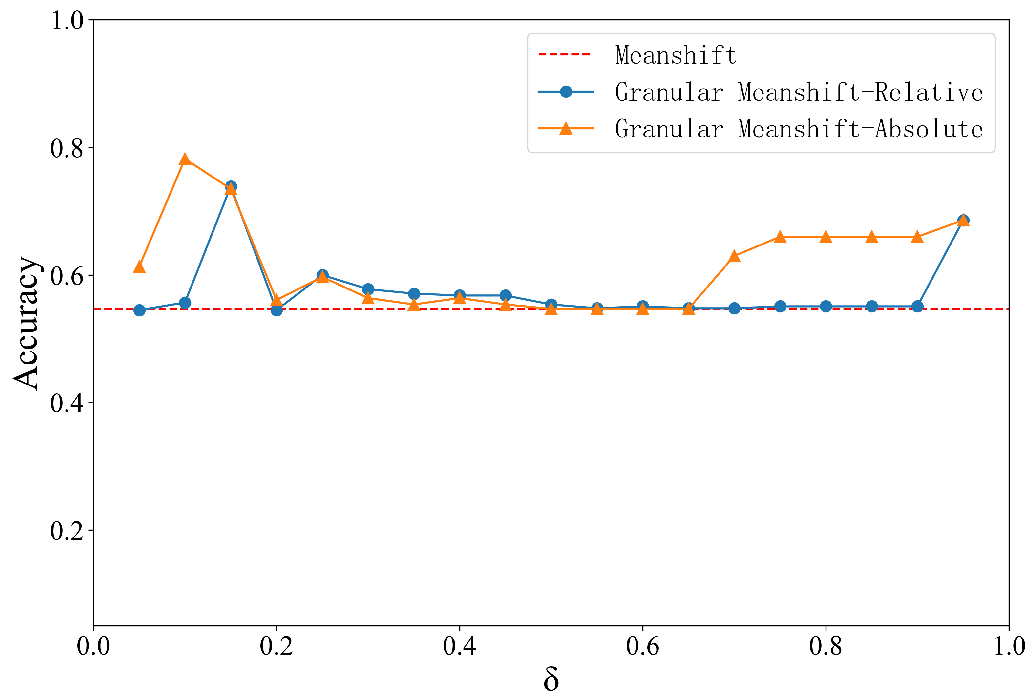
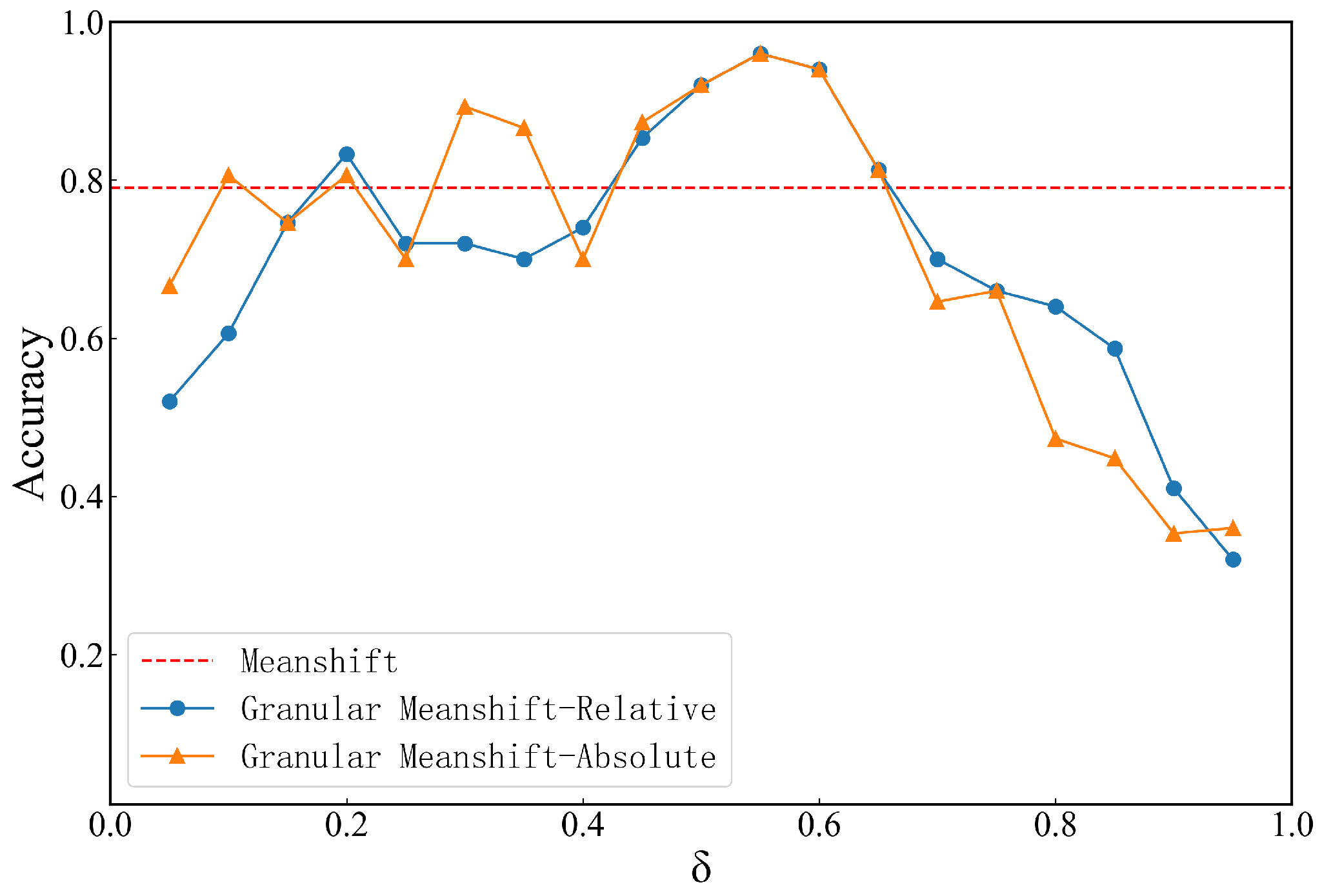
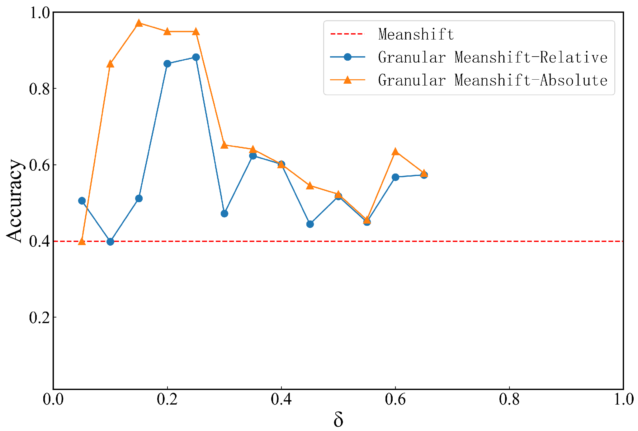
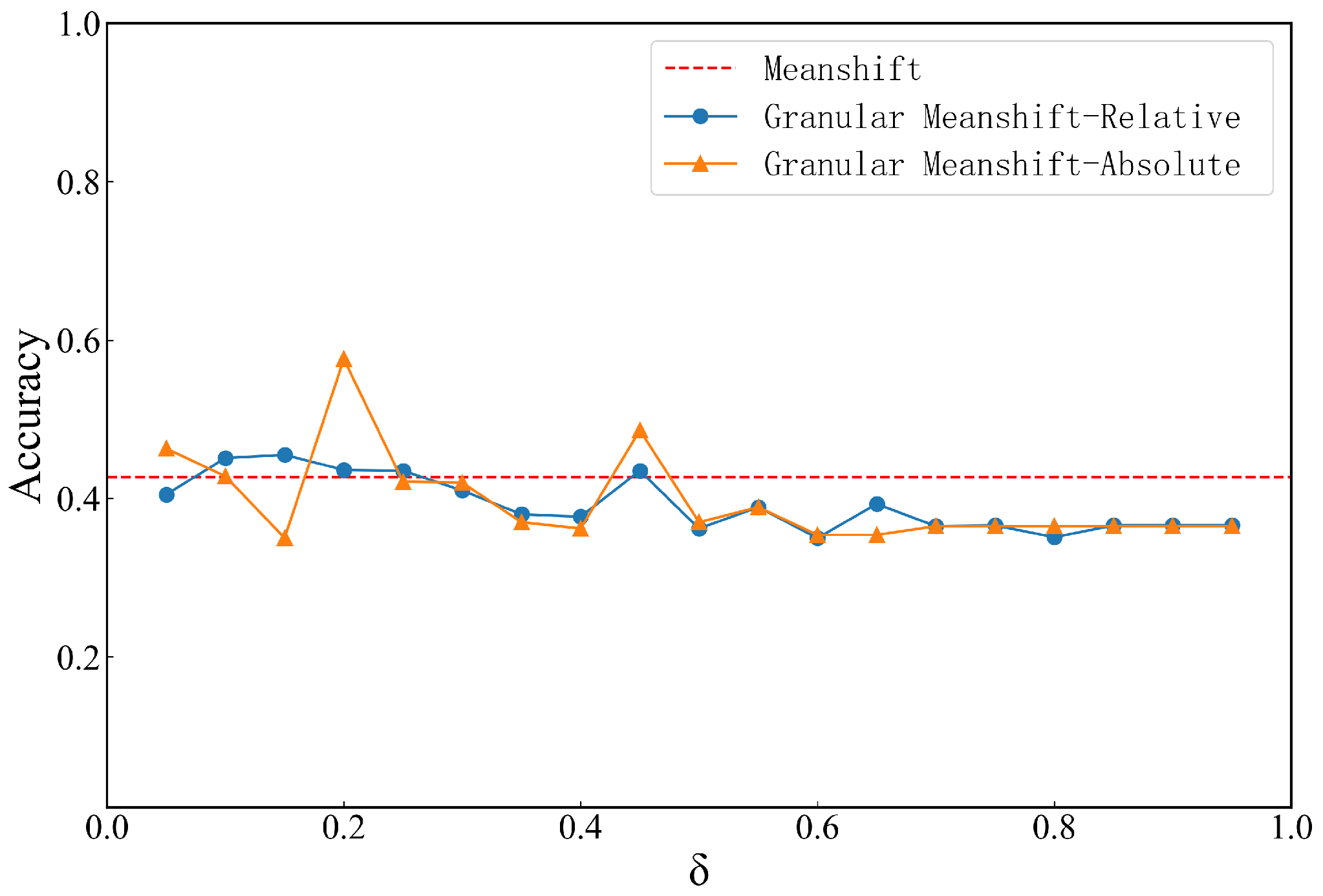
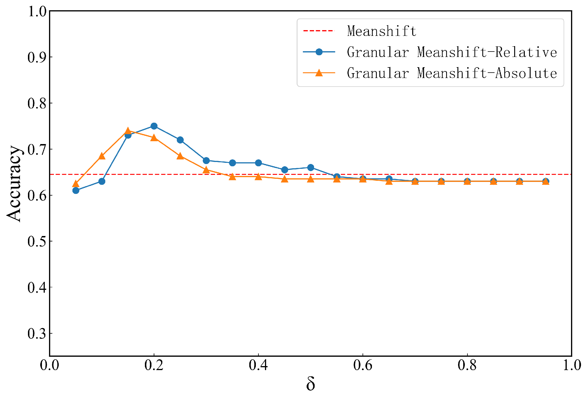
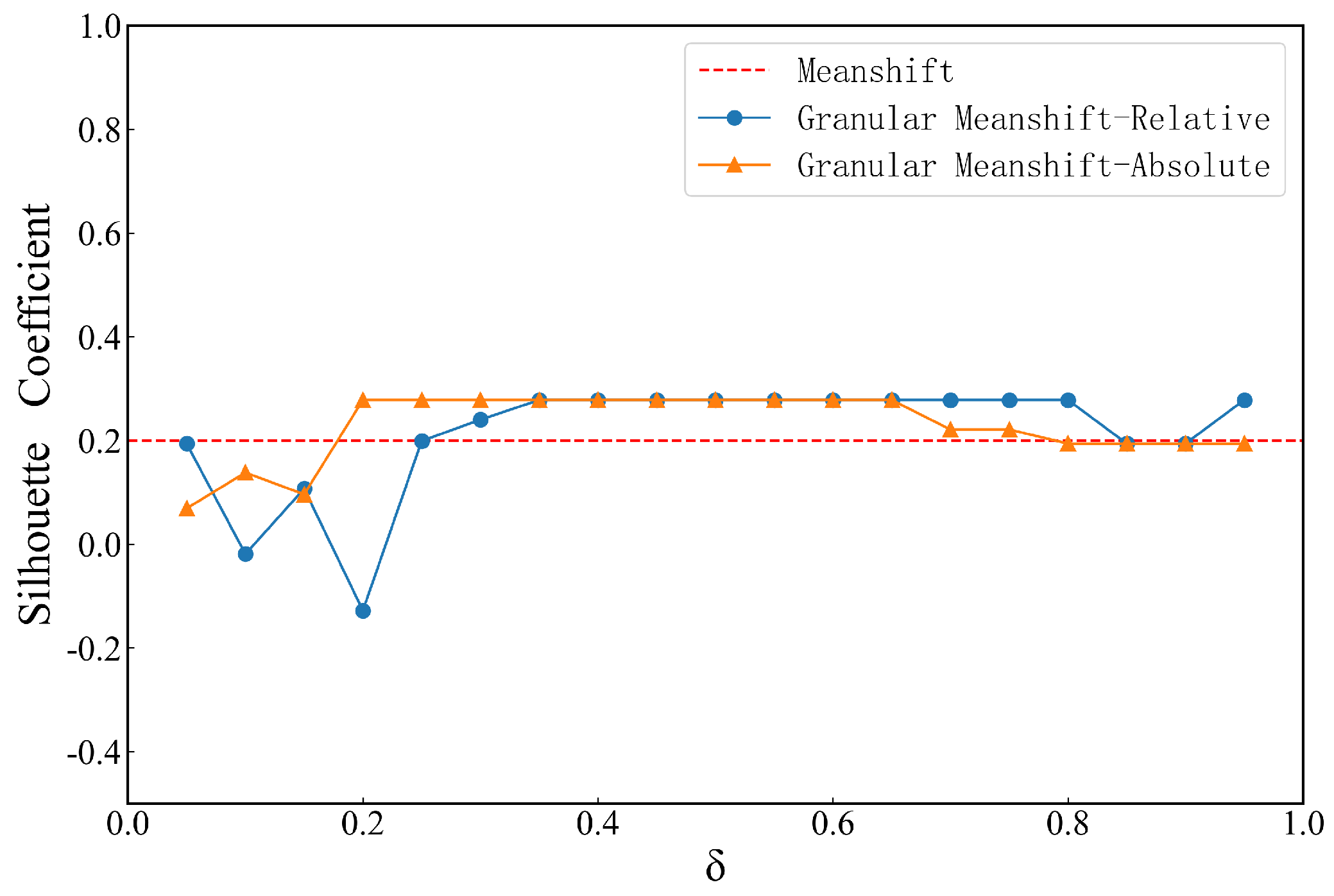
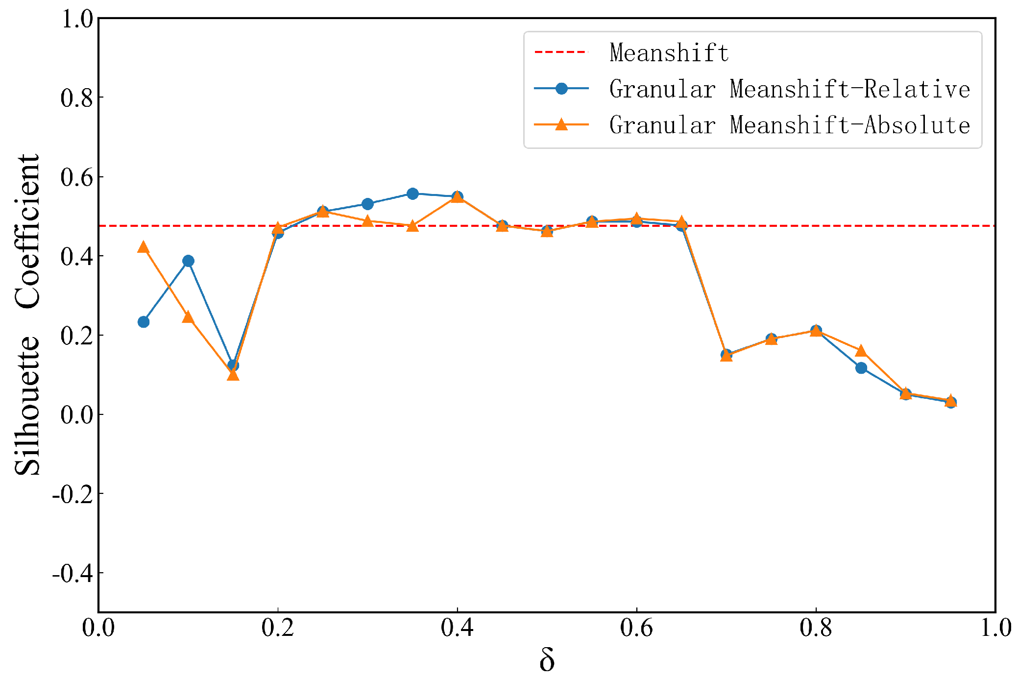
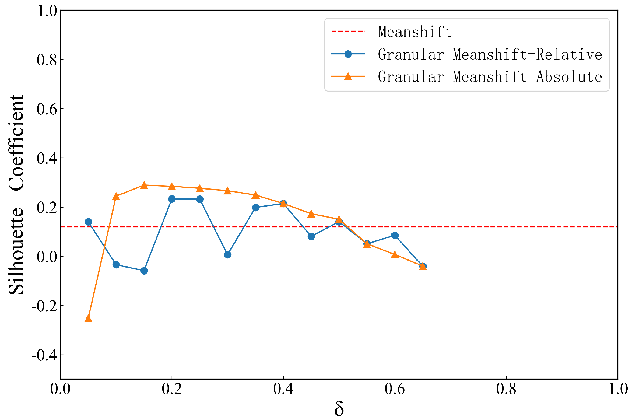
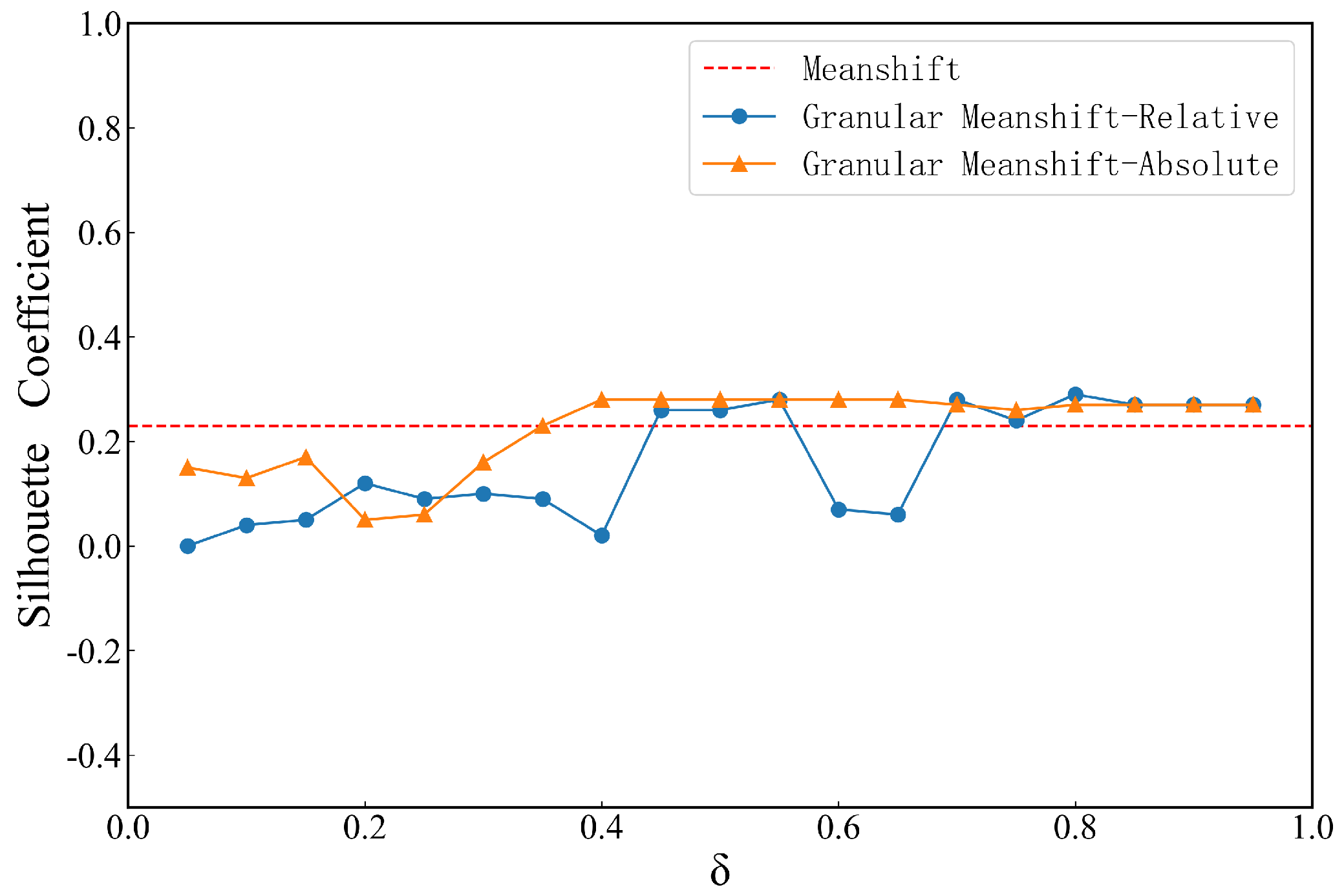
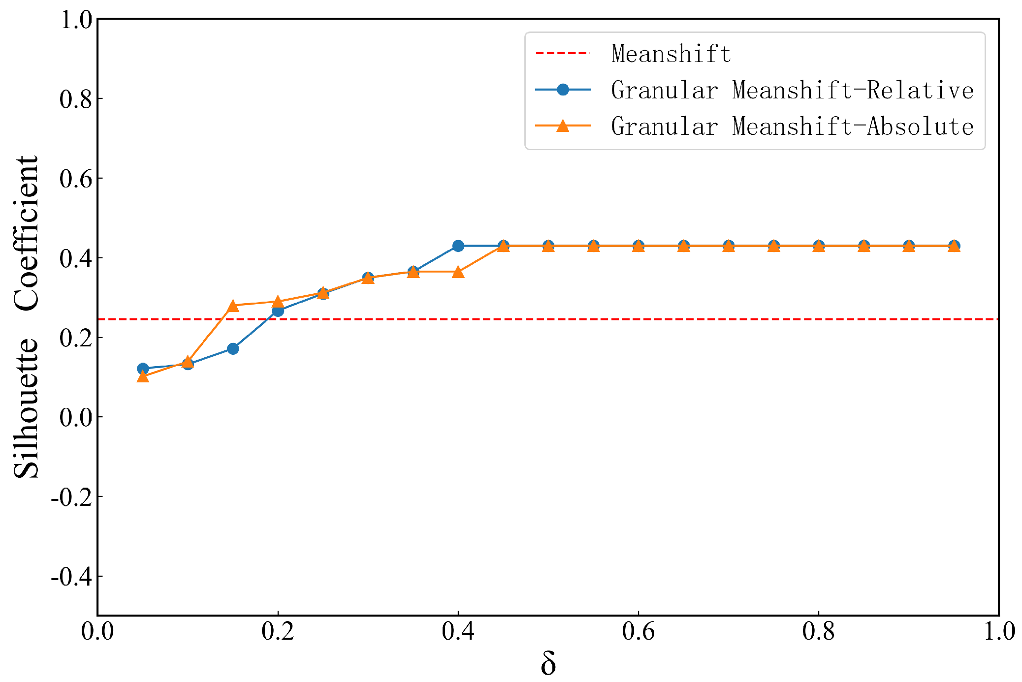
4.1. Effect of Neighborhood Granular Parameters

In the experiment, firstly the UCI datasets is granulated according to different NGP, then different neighborhood granular vectors are constructed, and finally the values of the granular meanshift clustering algorithm based on the granular vectors absolute and relative distances are, respectively, calculated by the granular meanshift in Section 3.3 above. Different granulation processes of neighborhood parameters construct different neighborhood granule vectors, which affect the final clustering results. To further explore the effect of the Neighborhood Granular Parameter (NGP) in the granular meanshift clustering algorithm, validation is performed on datasets with different NGPs. The Accuracy rate and SC are used as clustering performance evaluation indicators, and the clustered label results are compared with the actual labels. The experiments are conducted with an NGP of 0 to 1 interval of 0.05, and the experimental results for each UCI dataset with different NGPs are shown in Figure 1, Figure 2, Figure 3, Figure 4, Figure 5, Figure 6, Figure 7, Figure 8, Figure 9 and Figure 10.

As can be seen from Figure 1, the accuracy of the traditional Meanshift clustering algorithm is 0.54, and the highest accuracy of the granular meanshift clustering algorithm based the granular vectors absolute and relative distance is 0.73 and 0.78, respectively, in the Heart Disease dataset. The granular meanshift is poor when the NGP is in the 0.20 to 0.65, but is still larger than the corresponding accuracy value of traditional meanshift.

As can be seen from Figure 2, Figure 3, Figure 4 and Figure 5, when NGP changes in Iris, Wine, CMC, and Pim datasets, the trend in Accuracy values for granular meanshift based on the granular vectors absolute and relative distances is consistent. When NGP is too large or too small, the granular meanshift clustering algorithm has a large variation in clustering performance. The highest Accuracy index values for the Iris datasets are 0.96 and 0.96, respectively, when NGP is taken to be 0.55, to the granular meanshift based on both granular vectors distance. However, when NGP is larger than 0.70, the Accuracy index value of granular meanshift clustering algorithm drops precipitously, degrading the clustering performance of the algorithm. The values of NGP for the Wine dataset are 0.15 and 0.25; the maximum Accuracy for granular meanshift clustering algorithm based on the granular vectors absolute and relative distances is 0.97 and 0.88, respectively. When the NGP is below 0.20 or above 0.30, the Accuracy of granular meanshift declines, but it remained higher than that of traditional meanshift. If the value of NGP is greater than 0.65, then the granular meanshift cannot be used in the Wine dataset.

When we take NGP to be 0.20 and 0.10 in the CMC dataset, the corresponding largest Accuracy values of granular meanshift based on the granular vectors absolute and relative distances are 0.44 and 0.57, respectively. However, when the NGP is taken to be 0.15 and 0.20 for the Pim dataset, the corresponding Accuracy of granular meanshift based on the granular vectors absolute and relative distance are 0.75 and 0.74, respectively, which is better than the Accuracy values from the traditional meanshift. The experimental results for granular meanshift in the above datasets show that the granular meanshift outperforms traditional meanshift concerning the proper neighborhood metrics.

Figure 6 and Figure 10 show that in the Heart Disease and Pim datasets, the SC in granular meanshift is lower than the corresponding SC in traditional meanshift when the NGP is low, and when NGP is larger, the SC in granular meanshift remained largely unchanged, but is larger than the corresponding SC in traditional meanshift. In the Heart Disease dataset, the largest SC for granular meanshift at both granular vectors distances is 0.27 when the NGP value is taken to be 0.35. The highest SC for granular meanshift on the Pim dataset at both granular vector distances is 0.42 when the NGP value is taken to be 0.45.

In experiments with Iris, Wine, and CMC datasets, clustering performed poorly when neighborhood parameters are small or large from Figure 7, Figure 8 and Figure 9. For the Iris dataset, the SC value of traditional meanshift is 0.47, and the maximum SC values of granular meanshift based on granular vectors absolute and relative distance are 0.55 and 0.54, respectively, and the clustering performance of granular meanshift is better than that of the traditional meanshift for an NGP that is well suited to the task at hand. The value of SC in traditional meanshift for the Wine dataset is 0.11, and the maximum SC values of granular meanshift based on the granular vectors absolute and relative distance are 0.23 and 0.28, respectively, and the SC performs better than traditional meanshift. However, when NGP is greater, the granular meanshift is no longer fit to the Wine dataset. The traditional Meanshift has an SC value of 0.23 for the CMC dataset, while the granular meanshift based on granular vectors absolute and relative distance has a maximum SC of 0.285 and 0.288, respectively, when the value of NGP is taken to be 0.55.

As can be seen from Figure 1, Figure 2, Figure 3, Figure 4, Figure 5, Figure 6, Figure 7, Figure 8, Figure 9 and Figure 10, for different datasets with different data distributions, different NGPs affect the final clustering performance from the NGP perspective. In general, the Accuracy of granular meanshift is higher than the Accuracy of traditional Meanshift, which means that the Accuracy of granular meanshift is always greater than the Accuracy of traditional Meanshift by finding the appropriate neighborhood parameters. Compared to the traditional Meanshift, the granular meanshift can pre-granulate data before the algorithm starts. Using neighborhood granular vectors, the granular meanshift converges more quickly on linear and nonlinear datasets and has a high clustering performance.

4.2. Comparison Experiment with Traditional Clustering Algorithms

In this experiment, the granular meanshift based on relative distance and the granular meanshift clustering algorithm based on absolute distance will be verified with the K-means, Meanshift, Gaussian Mixture, Birch, and Agglomerative Clustering algorithms in the above five data sets. The three indicators of Accuracy, SC and FMI are used for comparison, the closer the value is to 1, the better the clustering performance. The results are shown in

Table 2. Comparison of algorithms on different datasets with Accuracy.

Dataset	Granular Meanshift Relative	Granular Meanshift Absolute	Meanshift	Kmeans	Gaussian Mixture	Birch	Agglomerative Clustering
CMC	0.576	0.455	0.4270	0.4372	0.4270	0.4276	0.4297
Iris	0.9667	0.96	0.7933	0.9666	0.9666	0.8666	0.8866
Heart Disease	0.782	0.739	0.547	0.719	0.719	0.544	0.679
Pim	0.74	0.75	0.645	0.625	0.675	0.645	0.64
Wine	0.97191	0.882	0.3988	0.9494	0.9606	0.6067	0.9775

,

Table 3. Comparison of algorithms on different datasets with Silhouette Coefficient.

Dataset	Granular Meanshift Relative	Granular Meanshift Absolute	Meanshift	Kmeans	Gaussian Mixture	Birch	Agglomerative Clustering
CMC	0.2889	0.2857	0.2316	0.2345	0.2959	0.2776	0.2963
Iris	0.5494	0.5578	0.4764	0.4507	0.4507	0.5061	0.5043
Heart Disease	0.278	0.278	0.2	0.251	0.251	0.215	0.213
Pim	0.4297	0.4297	0.2455	0.2268	0.1778	0.1765	0.1956
Wine	0.2891	0.2332	0.1194	0.3008	0.2993	0.281	0.2948

and

Table 4. Comparison of algorithms on different datasets with Fowlkes–Mallows Index.

Dataset	Granular Meanshift Relative	Granular Meanshift Absolute	Meanshift	Kmeans	Gaussian Mixture	Birch	Agglomerative Clustering
CMC	0.5685	0.5685	0.5171	0.3635	0.4356	0.4780	0.4303
Iris	0.9364	0.9232	0.7476	0.9355	0.9355	0.7946	0.8158
Heart Disease	0.7069	0.7069	0.7069	0.6191	0.6191	0.6127	0.6065
Pim	0.7257	0.7257	0.6800	0.5202	0.6086	0.5602	0.5526
Wine	0.9448	0.7937	0.5605	0.9026	0.9215	0.6799	0.9542

.

Table 2, Table 3 and Table 4 show the optimal test results of different clustering algorithms in the corresponding data sets and are marked in bold. Table 2 shows that when Accuracy is used as the performance evaluation index, the absolute distance-based granular meanshift clustering algorithm scores better than the other six clustering algorithms in the CMC, Iris, and Heart Disease datasets. In the Pim dataset, the scores of the relative distance-based granular meanshift clustering algorithm are better than the test results of the other six clustering algorithms. In addition, in the Wine dataset, the score of the granular meanshift clustering algorithm based on the absolute distance is better than that of the other five algorithms except for the Agglomerative Clustering algorithm; while the score of the granular meanshift clustering algorithm based on the relative distance is better than the Meanshift and Birch algorithms, but less than K-means, Gaussian Mixture and Agglomerative Clustering algorithms.

Table 3 shows that when SC is used as a performance evaluation index, the performance of the granular meanshift clustering algorithm based on absolute distance in the Heart Disease and Pim datasets is better than that of the other six clustering algorithms. In the Iris dataset, the scores of the relative distance-based granular meanshift clustering algorithm are better than those of the other six clustering algorithms. In the Wine dataset, the score of the granular meanshift clustering algorithm based on absolute distance is better than the other three clustering algorithms, but lower than that of Agglomerative Clustering, Gaussian Mixture, and K-means algorithm; while the performance of the granular meanshift clustering algorithm based on relative distance is only better than the Meanshift clustering algorithm. In the CMC dataset, the granular meanshift clustering algorithm based on two distances scores better than the other four clustering algorithms except for Gaussian Mixture and Agglomerative Clustering algorithms. It can be seen from Table 4 that in the above data sets, the granular meanshift algorithm also has superior performance in terms of FMI indicators.

4.3. Discussions

The clustering performance of granular meanshift is better than Meanshift and other clustering algorithms on multiple data sets in conclusion. In the Wine dataset, although the performance of granular meanshift is slightly lower than that of the Gaussian Mixture and Agglomerative Clustering algorithms, the gap is not large. Different from the traditional clustering algorithm, the granular meanshift uses neighborhood granulation technology to seek structural breakthroughs, which improves the clustering performance of the algorithm and makes the algorithm have better results in different types of datasets.

5. Conclusions

To address the problem that the traditional clustering algorithms have difficulty dealing with the set-based data and nonlinear data based on the Mahalanobis distance and Minkowski distance, we bring the theory of neighborhood granular computing into the clustering algorithm. First, we define the granular vectors according to the neighborhood granulation theory and propose two novel distance metrics for granular vectors. After that, we propose the neighborhood granular meanshift algorithm based on the granular vectors relative distance and the granular vectors absolute distance. Finally, the experiments illustrate that the granular meanshift clustering algorithm our proposed has better clustering performance than traditional clustering algorithms, with an average improvement of 10.4%, 7.5%, and 9.8% in the Accuracy, SC and FMI, respectively.

In future work, we will define more advanced granular vectors distance metrics to improve the performance of the clustering algorithm. Moreover, it is an interesting work to apply the proposed granular vectors relative metric and granular vectors absolute metric to other clustering algorithms.

References

1. Zadeh, L.A. Fuzzy sets. Inf. Control 1965, 8, 338–353. [Google Scholar] [CrossRef] [Green Version]
2. Pawlak, Z. Rough sets. Int. J. Inf. Comput. Sci. 1982, 11, 341–356. [Google Scholar] [CrossRef]
3. Yao, Y.Y. Relational interpretations of neighborhood operators and rough set approximation operators. Inform. Sci. 1998, 111, 239–259. [Google Scholar] [CrossRef] [Green Version]
4. Lin, T.Y. Data Mining: Granular Computing Approach. Lect. Notes Comput. Sci. 1999, 1574, 24–33. [Google Scholar]
5. Yager, R.R.; Filev, D. Operations for granular computing: Mixing words with numbers. In Proceedings of the 1998 IEEE International Conference on Fuzzy Systems, Anchorage, AK, USA, 4–9 May 1998; pp. 123–128. [Google Scholar]
6. Lin, T.Y.; Zadeh, L.A. Special issue on granular computing and data mining. Int. Intell. Syst. 2004, 19, 565–566. [Google Scholar] [CrossRef]
7. Lin, C.F.; Wang, S.D. Fuzzy support vector machines. IEEE Trans. Neural Netw. 2002, 3, 464–471. [Google Scholar]
8. Wang, G.Y.; Zhang, Q.H.; Ma, X.; Yang, Q.S. Granular computing models for knowledge uncertainty. J. Softw. 2011, 22, 676–694. [Google Scholar] [CrossRef]
9. Hu, Q.; Yu, D.; Liu, J.; Wu, C. Neighborhood rough set based heterogeneous feature subset selection. Inform. Sci. 2008, 178, 3577–3594. [Google Scholar] [CrossRef]
10. Miao, D.Q.; Fan, S.D. The calculation of knowledge granulation and its application. Syst. Eng.-Theory Pract. 2002, 22, 48–56. [Google Scholar]
11. Hu, Q.H.; Yu, D.R.; Xie, Z.X. Neighborhood classifiers. Expert Syst. Appl. 2008, 34, 866–876. [Google Scholar] [CrossRef]
12. Qian, Y.H.; Liang, J.Y.; Dang, C.Y. Incomplete multigranulation rough set. IEEE Trans. Syst. Man Cybern-Part A 2010, 40, 420–431. [Google Scholar] [CrossRef]
13. Miao, D.Q.; Xu, F.F.; Yao, Y.Y.; Wei, L. Set-theoretic formulation of granular computing. Chin. J. Comput. 2012, 35, 351–363. [Google Scholar] [CrossRef]
14. Qian, J.; Miao, D.Q.; Zhang, Z.H.; Yue, X. Parallel attribute reduction algorithms using MapReduce. Inform. Sci. 2014, 279, 671–690. [Google Scholar] [CrossRef]
15. Chen, Y.M.; Miao, D.Q.; Wang, R. A rough set approach to feature selection based on ant colony optimization. Pattern Recognit. Lett. 2010, 31, 226–233. [Google Scholar] [CrossRef]
16. Chen, Y.M.; Zhu, Q.; Xu, H. Finding rough set reducts with fish swarm algorithm. Knowl. Based Syst. 2015, 81, 22–29. [Google Scholar] [CrossRef]
17. Chen, Y.M.; Qin, N.; Li, W.; Xu, F. Granule structures, distances and measures in neighborhood systems. Knowl.-Based Syst. 2019, 165, 268–281. [Google Scholar] [CrossRef]
18. Lei, T.; Jia, X.; Zhang, Y.; Liu, S.; Meng, H.; Nandi, A.K. Superpixel-Based Fast Fuzzy C-Means Clustering for Color Image Segmentation. IEEE Trans. Fuzzy Syst. 2019, 27, 1753–1766. [Google Scholar] [CrossRef] [Green Version]
19. Zhou, J.; Pedrycz, W.; Wan, J.; Gao, C.; Lai, Z.-H.; Yue, X. Low-Rank Linear Embedding for Robust Clustering. IEEE Trans. Knowl. Data Eng. 2022. [Google Scholar] [CrossRef]
20. Zhou, J.; Lai, Z.; Miao, D.; Gao, C.; Yue, X. Multigranulation rough-fuzzy clustering based on shadowed sets. Inf. Sci. 2020, 507, 553–573. [Google Scholar] [CrossRef]
21. Fujita, H.; Gaeta, A.; Loia, V.; Orciuoli, F. Hypotheses analysis and assessment in counter-terrorism activities: A method based on OWA and fuzzy probabilistic rough sets. IEEE Trans. Fuzzy Syst. 2019, 28, 831–845. [Google Scholar] [CrossRef]
22. Yue, X.D.; Zhou, J.; Yao, Y.Y.; Miao, D.Q. Shadowed neighborhoods based on fuzzy rough transformation for three-way classification. IEEE Trans. Fuzzy Syst. 2020, 28, 978–991. [Google Scholar] [CrossRef]
23. Li, W.; Ma, X.; Chen, Y.; Dai, B.; Chen, R.; Tang, C.; Luo, Y.; Zhang, K. Random fuzzy granular decision tree. Math. Probl. Eng. 2021, 1–17. [Google Scholar] [CrossRef]
24. Kaburlasos, V.G.; Lytridis, C.; Vrochidou, E.; Bazinas, C.; Papakostas, G.A.; Lekova, A.; Bouattane, O.; Youssfi, M.; Hashimoto, T. Granule-Based-Classifier (GbC): A Lattice Computing Scheme Applied on Tree Data Structures. Mathematics 2021, 9, 2889. [Google Scholar] [CrossRef]
25. Chen, Y.M.; Zhu, S.Z.; Li, W.; Qin, N. Fuzzy granular convolutional classifiers. Fuzzy Sets Syst. 2021, 426, 145–162. [Google Scholar] [CrossRef]
26. He, L.J.; Chen, Y.M.; Wu, K.S. Fuzzy granular deep convolutional network with residual structures. Knowl.-Based Syst. 2022, 258, 109941. [Google Scholar] [CrossRef]
27. He, L.J.; Chen, Y.M.; Zhong, C.M.; Wu, K.S. Granular Elastic Network Regression with Stochastic Gradient Descent. Mathematics 2022, 10, 2628. [Google Scholar] [CrossRef]
28. Perez, G.A.; Villarraso, J.C. Identification through DNA Methylation and Artificial Intelligence Techniques. Mathematics 2021, 9, 2482. [Google Scholar] [CrossRef]
29. Fukunaga, K.; Hostetler, L. The estimation of the gradient of a density function, with applications in pattern recognition. IEEE Trans. Inform. Theory 1975, 21, 32–40. [Google Scholar] [CrossRef] [Green Version]
30. Chen, Y.Z. Mean shift, mode seeking, and clustering. IEEE Trans. Pattern Anal. Mach. Intell. 1995, 8, 790–799. [Google Scholar]
31. Comaniciu, D.; Meer, P. Mean shift: A robust approach toward feature space analysis. IEEE Trans. Pattern Anal. Mach. Intell. 2002, 24, 603–619. [Google Scholar] [CrossRef] [Green Version]
32. Wu, X.R.L.I.F.C.; Hu, Z.Y. Convergence of a mean shift algorithm. J. Softw. 2005, 16, 365–374. [Google Scholar]
33. Lai, J.; Wang, C. Kernel and graph: Two approaches for nonlinear competitive learning clusterin. Front. Electr. Electron. Eng. 2012, 7, 134–146. [Google Scholar] [CrossRef]
34. Chen, C.; Lin, K.Y.; Wang, C.D.; Liu, J.B.; Huang, D. CCMS: A nonlinear clustering method based on crowd movement and selection. Neurocomputing 2017, 269, 120–131. [Google Scholar] [CrossRef]
35. Qin, Y.; Yu, Z.L.; Wang, C.D.; Gu, Z.; Li, Y. A novel clustering method based on hybrid k-nearest-neighbor graph. Pattern Recognit. 2018, 74, 1–14. [Google Scholar] [CrossRef]
Figure 1. Effect of NGP with Accuracy on Heart Disease dataset.
Mathematics 11 00207 g001
Figure 2. Effect of NGP with Accuracy on Iris dataset.
Mathematics 11 00207 g002
Figure 3. Effect of NGP with Accuracy on Wine dataset.
Mathematics 11 00207 g003
Figure 4. Effect of NGP with Accuracy on CMC dataset.
Mathematics 11 00207 g004
Figure 5. Effect of NGP onwith Accuracy on Pim dataset.
Mathematics 11 00207 g005
Figure 6. Effect of NGP with Silhouette Coefficient on Heart dataset.
Mathematics 11 00207 g006
Figure 7. Effect of NGP with Silhouette Coefficient on Iris dataset.
Mathematics 11 00207 g007
Figure 8. Effect of NGP with Silhouette Coefficient on Wine dataset.
Mathematics 11 00207 g008
Figure 9. Effect of NGP with Silhouette Coefficient on CMC dataset.
Mathematics 11 00207 g009
Figure 10. Effect of NGP with Silhouette Coefficient on Pim dataset.
Mathematics 11 00207 g010