Open-Set Recognition Model Based on Negative-Class Sample Feature Enhancement Learning Algorithm

Abstract

In order to solve the problem that the F1-measure value and the AUROC value of some classical open-set classifier methods do not exceed 40% in high-openness scenarios, this paper proposes an algorithm combining negative-class feature enhancement learning and a Weibull distribution based on an extreme value theory representation method, which can effectively reduce the risk of open space in open-set scenarios. Firstly, the solution uses the negative-class sample feature enhancement learning algorithm to generate the negative sample point set of similar features and then compute the corresponding negative-class sample feature segmentation hypersphere. Secondly, the paired Weibull distributions from positive and negative samples are established based on the corresponding negative-class sample feature segmentation hypersphere of each class. Finally, solutions for non-linear multi-class classifications are constructed by using the Weibull and reverse Weibull distributions. Experiments on classic open datasets such as the open dataset of letter recognition, the Caltech256 open dataset, and the CIFAR100 open dataset show that when the openness is greater than 60%, the performance of the proposed method is significantly higher than other open-set support vector classifier algorithms, and the average is more than 7% higher.

1. Introduction

There are many classical closed-set classifier algorithms in machine learning, including the k-nearest neighbor algorithm, random forest algorithm, support vector machine, and deep neural network. These classifiers are designed to work in closed-set scenarios; in essence, that is, all test sample categories must be subsets of the categories used in training. However, when the class of a test sample does not belong to any class in the training set, the closed-set classifier often mistakenly classifies the sample into a similar class in the training set rather than directly rejecting it. In the open-set scenario, the recognition problem should consider four basic categories of classes as follows [1]:

• Known known classes (KKCs): the classes with distinctly labeled positive training samples.
• Known unknown classes (KUCs): labeled negative samples, but do not belong to any class.
• Unknown known classes (UKCs): classes with no available samples in training, but available side information such as semantic/attribute information.
• Unknown unknown classes (UUCs): classes without any information regarding them during training.

Therefore, classifiers in open-set scenarios must have such an ability: in the open-set scenario, new classes (UUC) that cannot be seen during training appear in the test, and the classifier is required to not only accurately classify KKCs but also effectively handle UUCs. Therefore, the classifier needs to have corresponding reject UUCs.

One way to solve the problem of open-set recognition is to use a closed-set classifier and input the test samples into the classifier to obtain a similarity score or, alternately, calculate the distance between the test samples and the most likely category in the feature space and apply a threshold to classify the similarity score or distance. The purpose of applying the threshold is to classify any test samples whose similarity score or distance is lower than the specified threshold as an unknown category [2,3,4]. Mendes Júnior et al. [4] showed that when the threshold is applied to the ratio of distance rather than the distance itself, better performance will be generated in open-set scenarios. However, at present, the selection of a threshold usually only depends on the knowledge of KKCs and simply uses a threshold to distinguish KKCs from UUCs, because existing models cannot directly model UUCs, which inevitably incurs risks due to lacking available information from UUCs.

Another method is to use kernel-based algorithms, rather than similarity-based algorithms, to project sample features into a unified feature space to build a decision hyperplane. For example, using the support vector data description (SVDD) [5] and one-class SVM [6] to calculate the corresponding decision function for each category and apply it to the entire training set as a rejection function [7,8]. This method is called a classification algorithm with the ability to reject.

The process is to establish an initial rejection stage to predict whether the input belongs to a certain training category (known or unknown). The classification stage is to use a multi-class binary classifier to classify test samples when the test samples belong to a known category. The kernel-based algorithms rely on a specific classification hyperplane for each known class so that when each function’s decision chooses to reject the test sample, the test sample will be classified as an unknown class. These algorithms aim to minimize the positive-class open space of each binary classifier [9,10]. In binary classification, positive-class open space refers to the feature space of positive-class samples. In multi-category scenarios, a similar concept also applies: known category open space (KLOS) [11,12], that is, a set of feature spaces of all known categories. However, in reality, with high openness, the algorithm based on the kernel operator still only relies on the features contained in KKCs to calculate the decision hyperplane. Although it can distinguish the known and unknown categories that are far away from each other, for the known and unknown categories that are close to each other, the decision plane will often incorrectly identify the unknown category as a known category or wrongly reject the known category as an unknown category.

The key to kernel-based models is to learn the invariant features of homologous classes [13,14] and exclude outlier samples. If the features of KKCs are augmented based on its invariant features, and the augmented features are taken as known unknown category samples, i.e., KUCs, then the KKCs and KUCs obtained through feature augmentation are taken as a training set, and the sample features are projected into a unified feature space using a kernel-based algorithm to build the decision hyperplane. This method can effectively improve the defect that traditional classifiers only rely on the features of KKCs for training. In the open-set scenario, this method analyzes the distribution of all category characteristics: when the category of the test set sample is unpredictable, that is, the test set may contain one or more unknown categories, and its actual distribution will eventually be approximate to the extreme value distribution [15]. For this reason, this paper proposes a classifier design scheme combining negative-class sample feature adversarial learning and an extreme Weibull distribution representation method. By constructing a segmentation hyperplane based on adversarial negative-class samples and positive-class samples, this method rejects the unknown-class samples that are far away from the known class. Considering that the data distribution of the test set will approach the extreme value distribution in the open-set scenario, the paired Weibull distribution is used to prevent the model from incorrectly identifying unknown-class samples or known-class samples that are close to known classes, to improve the F1-measure value and the AUROC value of the classifier. In this paper, experiments on classic open-set datasets such as the letter recognition open dataset, the Caltech256 open dataset, and the CIFAR100 open dataset show that the F1-measure value and the AUROC value of the algorithm proposed in this paper are significantly higher than those of other classic open-set classifiers when the openness is greater than 60%.

In summary, the contributions of this article are:

(1) We propose a novel open-set recognition algorithm called the Weibull tightly wrapping description (WTWD), which can perform negative-class sample feature adversarial learning and open-set recognition based on a paired Weibull distribution in a unified strategy.

(2) An experimental evaluation of WTWD in detection and multi-class open-set scenarios.

The rest of this paper is organized as follows: Section 2 mainly presents the algorithms that are related to this paper, including SVDTWDD and meta recognition. The objective function and optimization algorithm of WTWD are given in detail in Section 3. The experimental results on the letter recognition open dataset, the Caltech256 open dataset, and the CIFAR100 open dataset show the performance of WTWD in Section 4. Finally, Section 5 summarizes the full text.

2. Related work

2.1. Meta Recognition and Extreme Value Theory

The post-cognitive scoring analysis is an emerging cognitive system prediction paradigm, a form of meta-recognition [16,17]. Score analysis after the classification system generates a series of decision or similarity scores for the input sample instances. These scores are used as fitting predictors, which will determine whether the classification of the post-identification classifier is successful or not and output the probability of the class the sample instance belongs to. Thus, the prediction result will be based on the decision of the post-recognition classifier, not the original classification result.

Many classifiers replace the probability in the above definition with a more general “score”, for which the final maximum likelihood classifier produces the same classification result when the posterior probability function is monotonic with the score function. For the classifier, the threshold $t_0$ on the similarity probability or score s will be set as the boundary between positive- and negative-class samples. However, the choice of $t_0$ is usually done empirically. When $t_0$ falls on each tail of each population distribution, a false rejection (type II error: there is a test-sample class in the training set, but the test sample is falsely rejected as an unknown class) or false identification (type I error: where there are no test-sample classes in the training set, but the classifier misclassifies the test samples into known classes) would occur. Walter J et al. [16,17] proved that at the tail of each distribution, that is, at the boundary of the sample distribution, when there are enough samples and categories, sampling the first n scores will make the final result approach the extreme value distribution, or the Weibull distribution when the data is bounded. At this time, using the Weibull distribution as the posterior classification method can reduce the probability of false rejection and false identification, as shown in Figure 1. However, this method only considers the impact of the decision score at the boundary of the known category sample on the discriminator in the open-set scenario and does not improve the segmentation plane that divides the known category from the unknown category.

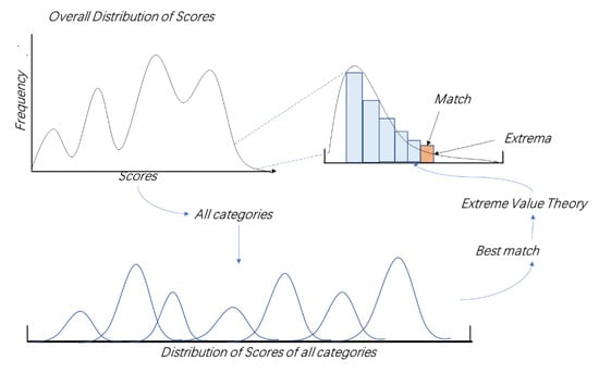
Figure 1. Sample score distribution generated by multi-class binary classifier.

2.2. Support Vector Domain Tightly Wrapping Description Design (SVDTWDD)

The classifier algorithm has made many excellent achievements in the past decade. Classifiers based on traditional machine learning methods and deep neural network methods have made great progress. However, in some special situations, due to the conflict between the sample distribution and decision surface, error recognition and error rejection will occur. To solve this problem, we need to design a classifier to make the feature area $C_{\omega }$ of samples of the same class $\omega$ determined by the classifier almost contain the actual feature area formed by all the sample points of class $\omega$ and not infringe on the feature area of other known classes or the feature space of unknown classes. Yang et al. [13] proposed using the nearest-neighbor points of each sample to calculate the compactness parameter, $\epsilon$, to ensure that the negative sample point set, which is derived from the positive sample feature area, only covers the original positive sample feature area. The new sample space is called the tightly wrapped point set, $I_k\left(C\right)$. We compute the negative-class sample feature segmentation hypersphere based on the tightly wrapped point set, $I_k\left(C\right)$, as shown in Figure 2.

Figure 2. The set of tight-wrapping points and tight-wrapping surfaces of feature domains. The blue points represent the positive sample, the green points represent the negative sample, and the red circles are support vectors.

It can be proved that the number of points of $I_k\left(C\right)$ shall not be less than the number of boundary points of the training set, $C$, and when $\epsilon$ is very small, the difference between the volume of $C$ and the volume of $I_k\left(C\right)$ is less than $2N{\left(2\eta +2\epsilon /\sqrt{rN}\right)}^{N-1}\left(\epsilon /\sqrt{rN}\right)$ and the resulting $I_k\left(C\right)$ can completely cover the training samples and reduce the space occupied by negative samples.

3. Proposed Method

The Weibull classifier uses extreme value theory to estimate the boundary probability. The open-set recognition problem itself conforms to the hypothesis of statistical extreme value theory (EVT) [15,18,19], which provides a quantitative probability method for the open-set recognition problem. The distribution of the decision score extreme values generated by any classification algorithm can be modeled using the extreme value theory. If the decision score has an upper bound, the distribution conforms to the reverse Weibull distribution, and its CDF is

$$P_{\psi }\left(y|F\left(x\right)\right)=e^{-{\left(\frac{-F\left(x\right)-v_{\psi }}{{\lambda }_{\psi }}\right)}^{k_{\psi }}}$$

(1)

If there is a lower bound, it conforms to Weibull distribution, and its CDF is

$$P_{\eta }\left(y|F\left(x\right)\right)=1-e^{-{\left(\frac{F\left(x\right)-v_{\eta }}{{\lambda }_{\eta }}\right)}^{k_{\eta }}}$$

(2)

where F(x) represents the sample score calculated from the decision curved surface, and $v_{\psi }, k_{\psi }, {\lambda }_{\psi }$ represent the location parameter, shape parameter, and scale parameter of the reverse Weibull distribution, respectively. Additionally, $v_{\eta }, k_{\eta }, {\lambda }_{\eta }$ represent the location parameter, shape parameter, and scale parameter of the Weibull distribution, respectively.

3.1. Construction Stage of Negative-Class Sample Feature Set

3.1.1. Optimization Algorithm for Compactness Parameter $\epsilon$ of Negative-Class Sample Features

There is a set of similar feature points collected from the similar feature space $T\subset R^N$ as $C$, which is a compact bounded convex set. There are $M$ points in $C$, $X_1,X_2,\dots ,X_M$; therefore, the compactness parameter $\epsilon$ optimization algorithm is as follows:

Step 1:

calculate sample point $X_j$ nearest-neighbor $N+1$points

$$\begin{array}{c}{j}_1=\mathit{arg}\underset{i\ne j}{min}\parallel X_j-X_i\parallel \\ j_2=\mathit{arg}\underset{i\ne j,j_1}{min}\parallel X_j-X_i\parallel \\ \dots \dots \\ j_{N+1}=\mathit{arg}\underset{i\ne j,j_1,\cdots ,j_N}{min}\parallel X_j-X_i\parallel \end{array}$$

(3)

Step 2:

calculate the maximum distance between sample point $X_j$ and the nearest neighbor

$$g\left(X_j\right)=\underset{i=j_1,\cdots ,j_{N+1}}{max}{X}_j-X_i$$

(4)

Step 3:

calculate the suboptimal estimate of the compactness parameter $\epsilon$

$$\epsilon \ge \sqrt{5.9N}\underset{1\le j\le M}{max}g\left(X_j\right)=\sqrt{5.9N}\underset{1\le j\le M}{max} \underset{i=j_1,\dots ,j_{N+1}}{\mathit{max}}\parallel X_j-X_i\parallel$$

(5)

3.1.2. Constructing Negative-Class Sample Feature Set

Using Equation (6) to construct $\epsilon /\sqrt{5.9N}-\epsilon$ negative sample feature set

$$I\left(C\right)=\left(C_{\epsilon }-C_{\frac{\epsilon }{\sqrt{5.9N}}}\right)\cap \left\{\left(X_{j1}\pm \epsilon ,\dots ,X_{ji}\pm \epsilon ,X_{jN}\pm \epsilon \right)\right|\left(X_{j1},X_{j2},\dots ,X_{jN}\right)ϵC\}$$

(6)

Step 1:

construct the hypersphere neighborhood discriminated functions of M points by Equation (7)

$$f_j\left(X\right)=\epsilon /\sqrt{5.9N}-\parallel X-X_j\parallel ,1\le j\le M$$

(7)

When $f_j\left(X\right)\ge 0$, $X$ lies in the hyperspherical neighborhood $\prod \left(X_j\right)$, the center of the hypersphere is $X_j$, and the radius is $\epsilon /\sqrt{5.9N}$.

Step 2:

for each point $X=\left(X_{j1},X_{j2},\dots ,X_{jN}\right),1\le j\le M$, can derive 2N points $\left(X_{j1}\pm \epsilon ,\dots ,X_{ji}\pm \epsilon ,X_{jN}\pm \epsilon \right)$.

Step 3:

check if each constructed point is in $\prod \left(X_j\right),1\le j\le M$. Then the set of all points, which are not in any $\prod \left(X_j\right)$, is the $\epsilon /\sqrt{5.9N}-\epsilon$ negative sample feature set.

3.1.3. Algorithm of Negative-Class Sample Segmentation Hypersphere

Negative-class sample points constructed by the negative-class sample feature set construction algorithm, $I_k\left(C\right)$, can be used as a training set to compute the negative-class sample segmentation hypersphere based on the kernel operator [20].

The point inside the small hypersphere is the corresponding point of the transformation from the midpoint of C to the high-dimensional space, and the point outside the large hypersphere is the point in $I_k\left(C\right)$ that is transformed to the corresponding point in the high-dimensional space. Our goal is to find a suitable transformation so that the mini hypersphere contains almost all the points and r is minimized, that is, ${\rho }^2$ is maximized. Thus, the original space surface corresponding to the small hypersphere in high-dimensional space is the negative-class sample feature segmentation surface of C.

C is the center of a high-dimensional space. We establish the following optimization model and construct the negative-class sample feature segmentation hypersphere by solving the optimization solution [21].

$$\begin{array}{c}\underset{r,c,\rho ,\epsilon }{\mathit{min}}{r}^2-v{\rho }^2+\frac{1}{v_1{m}_1}{\displaystyle \sum _{i=1}^{m_1}}{\epsilon }_i+\frac{1}{v_2{m}_2}{\displaystyle \sum _{j=m_1+1}^n}{\epsilon }_j\\ s.t.{\left|\left|\varphi \left(X_i\right)-c\right|\right|}^2 \le r^2+{\epsilon }_i ,1\le i\le m_1 ,\\ {\left|\left|\varphi \left(X_i\right)-c\right|\right|}^2 \ge r^2+{\rho }^2-{\epsilon }_j ,m_1\le j\le n ,\\ 0\le {\epsilon }_k,1\le k\le n\end{array}$$

(8)

where ${\epsilon }_i$, ${\epsilon }_j$ are slacking variables, and $\frac{1}{v_1{m}_1}$, $\frac{1}{v_2{m}_2}$ are punishment terms. To solve this optimization problem, we utilize the Lagrange function as:

$$\begin{array}{c}L\left(r,c,\xi ,\alpha ,\beta \right)=r^2-{\rho }^2+\frac{1}{{\upsilon }_1{m}_1}{\displaystyle \sum _{i=1}^{m_1}}{\xi }_i+\frac{1}{{\upsilon }_2{m}_2}{\displaystyle \sum _{j=1}^n}{\xi }_j\\ +{\displaystyle \sum _{i=1}^{m_1}}{\alpha }_i\left({\parallel \varphi \left(X_i\right)-c\parallel }^2-r^2-{\xi }_i\right)\\ -{{\displaystyle \sum }}_{j=m_1+1}^n{\alpha }_j\left({\parallel \varphi \left(X_i\right)-c\parallel }^2-r^2-{\rho }^2+{\xi }_j\right)-{{\displaystyle \sum }}_{k=1}^n{\beta }_k{\xi }_k \end{array}$$

(9)

The optima should satisfy the following conditions:

$$\frac{\partial L}{\partial r}=2r\left(1-{{\displaystyle \sum }}_{i=1}^n{\alpha }_i{y}_i\right)=0$$

(10)

$$\frac{\partial L}{\partial \rho }=2\rho \left(-\upsilon +{{\displaystyle \sum }}_{j=m_1+1}^n{\alpha }_i{y}_i\right)=0$$

(11)

$$\frac{\partial L}{\partial {\xi }_i}=\frac{1}{{\upsilon }_1{m}_1}-{\alpha }_i-{\beta }_i=0,1\le i\le m_1$$

(12)

$$\frac{\partial L}{\partial {\xi }_j}=\frac{1}{{\upsilon }_2{m}_2}-{\alpha }_j-{\beta }_j=0,m_1+1\le j\le n$$

(13)

$$\frac{\partial L}{\partial c}=2c{{\displaystyle \sum }}_{i=1}^n{\alpha }_i{y}_i-2{{\displaystyle \sum }}_{i=1}^n{\alpha }_i{y}_i\varphi (X_i)=0$$

(14)

As a result, we can obtain:

$$c=\frac{{{\displaystyle \sum }}_{i=1}^n{\alpha }_i{y}_i\varphi \left(X_i\right)}{{{\displaystyle \sum }}_{i=1}^n{\alpha }_i{y}_i}={{\displaystyle \sum }}_{i=1}^n{\alpha }_i{y}_i\varphi (X_i)$$

(15)

The dual problem is as follows:

$$\begin{array}{c}\underset{\alpha }{max}{\displaystyle \sum _{i=1}^n}{\alpha }_i{y}_i\varphi (X_i)\cdot \varphi \left(X_i\right)-{\displaystyle \sum _{i=1}^n}{\displaystyle \sum _{j=1}^n}{\alpha }_i{\alpha }_j{y}_i{y}_j\varphi \left(X_i\right)\cdot \varphi \left(X_j\right)\\ s.t.0\le {\alpha }_i\le \frac{1}{{\upsilon }_1{m}_1},1\le i\le m_1\\ 0\le {\alpha }_j\le \frac{1}{{\upsilon }_2{m}_2},m_1+1\le j\le n\\ {\displaystyle \sum _{i=1}^n}{\alpha }_i{y}_i=1\\ {{\displaystyle \sum }}_{i=1}^n{\alpha }_i=3v+1\end{array}$$

(16)

Using $K\left(X_i,X_j\right)$ to replace $\varphi \left(X_i\right)\cdot \varphi \left(X_j\right)$, we have Equation (17) based on the kernel function

$$\begin{array}{c}\underset{\alpha }{max}{\displaystyle \sum _{i=1}^n}{\alpha }_i{y}_{i}k(X_i,X_i)-{\displaystyle \sum _{i=1}^n}{\displaystyle \sum _{j=1}^n}{\alpha }_i{\alpha }_j{y}_i{y}_{j}k(X_i,X_j)\\ s.t.0\le {\alpha }_i\le \frac{1}{{\upsilon }_1{m}_1},1\le i\le m_1\\ 0\le {\alpha }_j\le \frac{1}{{\upsilon }_2{m}_2},m_1+1\le j\le n\\ {\displaystyle \sum _{i=1}^n}{\alpha }_i{y}_i=1\\ {{\displaystyle \sum }}_{i=1}^n{\alpha }_i=2\upsilon +1\end{array}$$

(17)

The dual problem is a quadratic programming problem, which can be solved by various algorithms aimed at solving quadratic programming problems, such as the sequential minimum optimization (SMO) algorithm.

After solving the above problems, in order to find $r$, ${\rho }^2$, and $r^2+{\rho }^2$, consider two sets

$$S_1=\{x_i\left|0\right.<{\alpha }_i<\frac{1}{{\upsilon }_1{m}_1},1\le i\le m_1\}$$

(18)

$$S_2=\{x_j\left|0\right.<{\alpha }_j<\frac{1}{{\upsilon }_2{m}_2},m_1+1\le j\le n\}$$

(19)

Let $n_1=\left|S_1\right|,n_2=\left|S_2\right|,$ by KKT conditions, we have

$$r^2=\frac{1}{n_1}{P}_1,{\rho }^2=\frac{1}{n_2}{P}_2-\frac{1}{n_1}{P}_1$$

(20)

where

$$\begin{array}{c}{P}_1={\displaystyle \sum _{x_i\in S_1}}{\parallel \varphi \left(X_i\right)-c\parallel }^2\\ ={{\displaystyle \sum }}_{x_i\in S_1}(k(X_i,X_i)-2{{\displaystyle \sum }}_{k=1}^n{\alpha }_k{y}_{k}k(X_i,X_k)+⟨c,c⟩)\end{array}$$

(21)

$$\begin{array}{c}{P}_2={\displaystyle \sum _{x_j\in S_2}}{\parallel \varphi \left(X_i\right)-c\parallel }^2\\ ={{\displaystyle \sum }}_{x_j\in S_2}(k\left(X_j,X_j\right)-2{{\displaystyle \sum }}_{k=1}^n{\alpha }_k{y}_{k}k\left(X_j,X_k\right)+⟨c,c⟩)\end{array}$$

(22)

$$⟨c,c⟩=⟨{{\displaystyle \sum }}_{i=1}^n{\alpha }_i{y}_i\varphi \left(X_i\right),{{\displaystyle \sum }}_{j=1}^n{\alpha }_j{y}_j\varphi \left(X_j\right)⟩={{\displaystyle \sum }}_{i=1}^n{{\displaystyle \sum }}_{j=1}^n{\alpha }_i{\alpha }_j{y}_i{y}_{j}k\left(X_i,X_j\right)$$

(23)

The decision function is

$$f\left(x\right)=\mathit{sgn}(r^2-{\parallel \varphi \left(X_i\right)-c\parallel }^2)=\mathit{sgn}(r^2+2{{\displaystyle \sum }}_{k=1}^n{\alpha }_k{y}_{k}k\left(X,X_k\right)-k\left(X,X\right)-⟨c,c⟩)$$

(24)

The classification decision hypersphere is $W$:

$$r^2-{\parallel \varphi \left(X_i\right)-c\parallel }^2=r^2+2{{\displaystyle \sum }}_{k=1}^n{\alpha }_k{y}_{k}k\left(X,X_k\right)-k\left(X,X\right)-⟨c,c⟩=0$$

(25)

3.2. Probability Calibration

Discriminative trained classifiers trained by the above algorithm can have very good closed-set performance. However, a good discriminative classifier in open-set scenarios should have no basis for prediction when the test sample is UUCs; thus, to improve the accuracy, we seek to combine the probabilities computed by both discriminative hyperplanes. Recent work has shown that the open-set recognition problem itself is consistent with the assumptions of statistical extreme value theory (EVT); therefore, we apply the EVT concept separately to the positive and negative scores from the negative-class sample hypersphere segmentation algorithm, and a reverse Weibull distribution is justified for the largest scores from the negative examples because they are bounded from above. Weibull is the expected distribution for the smallest scores from the positive examples because they are bounded from below.

The Weibull CDF derived from the match data is Equation (26):

$$P_{\eta }\left(y|W_i\left(x\right)\right)=1-e^{-{\left(\frac{W_i\left(x\right)-v_{\eta i}}{{\lambda }_{\eta i}}\right)}^{k_{\eta i}}}$$

(26)

and the reverse Weibull CDF derived from the non-match data, which is equivalent to rejecting the Weibull fitting on the non-match data, is Equation (27)

$$P_{\psi }\left(y|W_i\left(x\right)\right)=e^{-{\left(\frac{-W_i\left(x\right)-v_{\psi i}}{{\lambda }_{\psi i}}\right)}^{k_{\psi i}}}$$

(27)

The product of $P_{\eta }$ and $P_{\psi }$ represents the probability that the input comes from a positive class and not from any of the known negative class. In a closed-set scenario, using only $P_{\eta }$ indicates that the probability of positive samples is obviously better, because $P_{\eta }$ only uses positive data; however, because there are UUCs in the open-set scenario, and we cannot accurately model the unknown categories, $P_{\psi }$ should generally rely on other characteristics of non-negative samples for adjustment. At the same time, we note that the estimators are not completely conditional independent because they share the basic SVM discrimination structure, which is valid only when the input comes from a known category. Based on this deficiency, we use the negative sample feature enhancement learning algorithm of the same kind of feature set to assist in constructing the negative sample feature segmentation hypersphere. For a given class, $X_i$, the derived negative sample point set with the tight-wrapping property can fit a more accurate Weibull probability distribution function and reverse Weibull probability distribution function.

Algorithm 1 gives the concrete steps of WTWD:

Algorithm 1: WTWD

Input: training databases $X_i={\left\{x_{ij}\right\}}_{j=1}^n$ and label information $Y_i,i=1,\dots M$, test sample $x_t.$Open-set threshold ${\delta }_R$. 1. Optimization of compactness parameter $\epsilon$ by Equation (5). 2. Construct negative-class sample feature set by Equation (6). 3. Solve the negative-class sample segmentation hypersphere $W\left(X_i\right),$ and compute decision scores $S_{x_{ij}}$ of $x_{ij}$ by Equations (24) and (25). 4. Compute the paired Weibull distribution corresponding to each category，get location parameter, shape parameter, and scale parameter of Weibull distribution and reverse Weibull distribution respectively, $P=\left[v_{\eta i},k_{\eta i},{\lambda }_{\eta i},v_{\psi i},k_{\psi i},{\lambda }_{\psi i}\right],i=1,\dots M$. 5. Input test sample, $x_t$, use $W_i\left(x_t\right),i=1,\dots M$ to calculate decision scores $S_{x_t}$ for each category. Calculate probability of Weibull distribution $P_{\eta }$ and probability of reverse Weibull distribution $P_{\psi }$ for each category.    $Fori=1:M$        $if{S}_{x_t}>v_{\eta i}$,            $P_{\eta i}=1-e^{-{\left(\frac{S_{x_t}-v_{\eta i}}{{\lambda }_{\eta i}}\right)}^{k_{\eta i}}}$,        $else{P}_{\eta i}=0$.        $if-S_{x_t}>v_{\psi i},$            $P_{\psi i}=e^{-{\left(\frac{-S_{x_t}-v_{\psi }}{{\lambda }_{\psi }}\right)}^{k_{\psi }}},$        $else{P}_{\psi i}=0$     $end$     $i^{*}=\underset{i}{argmax}\left(P_{\eta i}\times P_{\psi i}\right)$     $if\left(P_{\eta i^{*}}\times P_{\psi i^{*}}\right)<{\delta }_R$        $i^{*}=0\mathrm{i}.\mathrm{e}.,x_t$ belongs to UUCs. 6. Output: classification result $i^{*}$ of test sample $x_t$

4. Experiment and Discussion

In order to verify the effectiveness of the WTWD algorithm, we first introduce three experimental databases, including the letter recognition open dataset [22], the Caltech256 open dataset [23], and the CIFAR100 open dataset [24]. Then, we provide evaluation indexes to evaluate the effects of different algorithms. We select several classical open-set recognition algorithms for performance comparison, including SVDD [5], TNN [8], WSVM [18], EVM [19], OSSVM [25], OnevsSet SVM [26], and Resnet [27]. Finally, for each database, we give the experimental results and corresponding analysis.

4.1. Databases and Setting

As shown in Figure 3, the letter recognition open dataset database involves 26 different classes, including all letter classes, all of which have 16 numerical attributes. These attributes represent primitive statistical features of the pixel distribution.

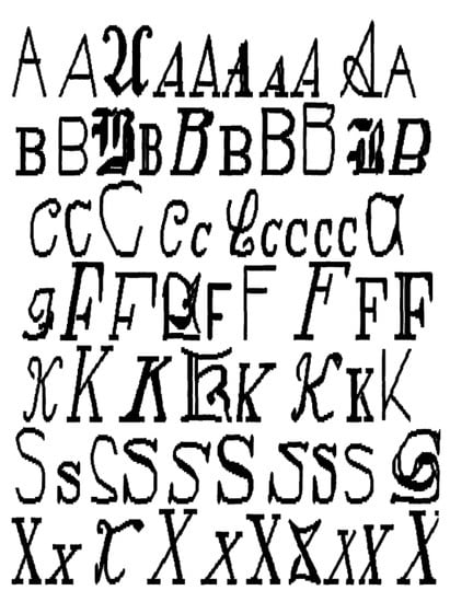
Figure 3. Examples of letter recognition open dataset.

In order to further test the performance of the algorithm in the actual scenarios, we chose the Caltech256 open dataset to verify the effectiveness of the WTWD algorithm and compared it with other classic open-set recognition algorithms. As shown in Figure 4, the Caltech256 open database includes 256 different classes, with each category containing over 80 pictures. We chose 20 images, 40 images, 60 images, and 80 images, respectively, as the training set and 20 images as the test set for each category, with 60 categories, 50 categories, and 40 categories selected as training sets, so the corresponding openness equals 0.3837, 0.42, and 0.48, respectively. The test set includes all categories of the Caltech 256 open dataset.

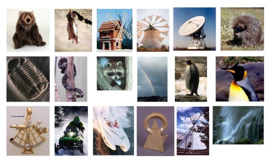
Figure 4. Examples of Caltech256 open dataset.

When the openness is extremely high and the resolution is lower, the performance of the algorithm will be greatly affected, so we chose the CIFAR100 open dataset to verify the effectiveness of the WTWD algorithm in extremely high-openness scenarios. As shown in Figure 5, the CIFAR100 open dataset includes 100 different classes, each class has 600 pictures, and the size of each picture is 32 × 32 RGB. We chose 200 images, 400 images, and 600 images, respectively, as the training set and 100 images as the test set for each category, with 10 categories selected as training sets, so the corresponding openness is about 0.6. The test set includes all categories of the CIFAR100 open dataset.

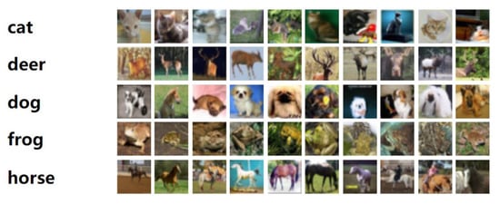
Figure 5. Examples of CIFAR100 open dataset.

4.2. Experiments and Results

4.2.1. Experiments on the Letter Recognition Open Dataset

In this section, we test the proposed algorithm on the letter recognition open dataset; the data distribution of the letter recognition open dataset is shown in Figure 6a.

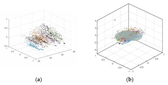
Figure 6. (a) Letter recognition open dataset data distribution. (b) Hypersphere constructed by SVDD.

As shown in Figure 6a, the black point set represents the sample point set of UUCs, while the colored point set represents the sample point set of KKCs. It can be seen that in the open-set scenario, the sample point set of unknown categories and the sample point set of known categories are mixed together. Figure 6b shows the decision hypersphere constructed by the support vector domain description method (SVDD) in the open-set scenario. Since the traditional classifier only trains the decision surface based on the sample point set of known categories, the decision surface will incorrectly identify the sample point set of unknown categories as the sample point set of a known category or wrongly reject the sample point set of a known category.

The area under the receiver operating characteristic curve (AUROC) and F1-measure were used for performance evaluation. AUROC is a measure of classifier performance. It reflects the performance of the classifier by the area between the receiver operating characteristic curve and the coordinate axis. AUROC is a value between 0 and 1. When the AUROC value is close to 1, it means that the classifier can better classify positive and negative samples. The F1-measure combines the precision, R, and recall, P. Both of them are widely used to test the performance of open-set recognition models. The F1-measure is defined as follows

$$F-measure=\frac{2\times P\times R}{P+R}$$

(28)

$$P=\frac{TP }{TP+FP} , R=\frac{TP}{TP+FN}$$

(29)

In open-set identification, openness is usually used to quantify open space risks [20], and openness is defined as:

$$openness=1-\sqrt{\frac{2\times C_T}{C_T+C_E}}$$

(30)

$C_T$ represents the number of categories of training set, and $C_E$ represents the number of categories in the test set; when $C_T=C_E$, open-set recognition will be converted to closed-set recognition. The algorithm rejection threshold used in this paper is ${\delta }_R=0.5\times openness$.

It can be seen from Figure 7a that compared with the other classifiers, the AUROC value of our proposed method under the closed-set condition is higher than the other classifiers but lower than SVDD. With a rapid increase in openness, the AUROC values of the following classifiers decrease rapidly: SVDD algorithm, TNN algorithm, and OnevsSet SVM. Additionally, the open-set classifiers, WSVM and OSSVM, have a certain degree of decline, but the AUROC of our proposed method is still relatively stable, indicating that this algorithm is less affected by open space risks. When the openness equals 0.6, the AUROC value of our proposed method still exceeds 90%, and the AUROC value of our proposed method is 14.7912% higher than SVDD and 8.9439% higher than WSVM.

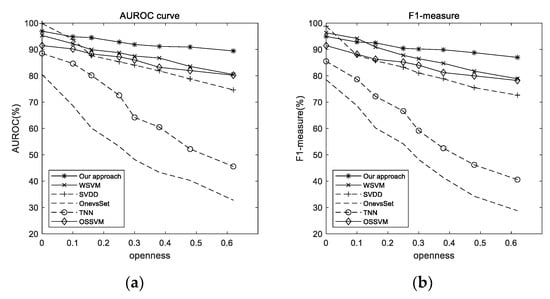
Figure 7. AUROC and F1-measure with increasing openness: (a) AUROC and (b) F1-measure.

Figure 7b shows the ability of our proposed method to correctly classify known category samples when it correctly rejects unknown category samples. When openness equals 0, the F1-measure reflects the ability of algorithms to classify correctly in the closed-set scenario. The best performance is from SVDD, which uses a segmentation hypersphere to classify. We believe it is rational to integrate the idea of a hypersphere to classify UUCs and KKCs, and the experimental results support this point of view. When the openness is 0.6, the F1-measure value of our proposed method equals 86.9563%, which is 14.3343% higher than SVDD and 8.1211% higher than WSVM. The results show that our proposed method has better classification performance in open-set scenarios; therefore, it is necessary to consider using a negative-class sample during training and a Weibull distribution to prevent the model from wrongly rejecting KKCs as UUCs or wrongly classifying UUCs as KKCs in open-set scenarios.

4.2.2. Experiments on Caltech256 Open Dataset

Different from the letter recognition open dataset, the Caltech256 open dataset consists of multi-class RGB images, and each image has meaningless background noise; therefore, we use ResNet18 to extract efficient features to verify the classification performance of our proposed method in the real scenario. We use a 48-dimension tensor to replace the original RGB image [28,29].

As shown in Figure 8, in the real scenario with an openness equal to 0.38, the F1-measure value and the AUROC value of the proposed algorithm are 3.1112% and 6.14% higher than those of WSVM and OSSVM, respectively. In the real scenario with an openness equal to 0.48, the F1-measure value and the AUROC value of the proposed algorithm are 7.3177% and 8.5182% higher than those of WSVM and OSSVM, respectively.

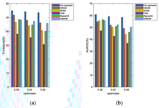
Figure 8. AUROC and F1-measure for open-set multi-class recognition in high-openness scenario: (a) F1-measure and (b) AUROC.

According to Algorithm 1, when sample $X$ belongs to a known category, $X_i$, the decision score calculated by the corresponding decision hypersphere, $W_i\left(X\right)$, is positive, while the other decision hypersphere, $W_j\left(X\right),j=1\dots M,j\ne i$, calculates a negative decision score. Thus, its corresponding Weibull distribution and reverse Weibull distribution are also unique. When sample $X$ is in the decision hypersphere of multiple known categories at the same time, since the probability of sample $X$ belonging to the known category $X_i$ is positively correlated to the decision score, sample $X$ is classified as the category with the largest product of the paired Weibull distribution, corresponding to $W_i\left(X\right)$. When the sample does not belong to any of the known categories, the model cannot find a matching pair of Weibull distributions; that is, the probability of all Weibull distributions equals 0 or does not exceed the threshold, so it is judged as an unknown category. Therefore, multiple paired Weibull distributions enable the model to further judge the samples which are in the decision hypersphere of multiple known categories at the same time.

As shown in Figure 9, we set different numbers of images as the training set to verify the robustness of the algorithm, and for an openness equal to 0.48, our proposed algorithm has a higher F1-measure and AUROC value under different numbers of training samples. Due to the use of negative samples to calculate the decision surface during the training phase, the F1-measure of our proposed method is still around 50%, whereas the other algorithms are more susceptible to the number of training samples.

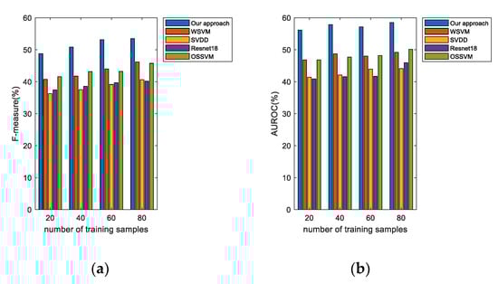
Figure 9. AUROC and F1-measure, when openness equals 0.48, for open-set multi-class recognition using different numbers of training samples on Caltech256 open dataset: (a) F1-measure and (b) AUROC.

In real scenarios, both high openness and insufficient training samples can be problems during model application. Segmentation of hyperspheres constructed by negative sample features and establishment of the corresponding paired Weibull distribution can effectively increase the anti-interference ability of the model to negative samples. Therefore, in the real scenario with higher openness, the recognition performance of the proposed algorithm declines slowly and tends to be stable.

4.2.3. Experiments on CIFAR100 Open Dataset

In the real scenario with high openness, we select the CIFAR100 open dataset. After feature extraction, the CIFAR100 open dataset dimension is $48\times 60,000$. We chose 10 classes as the training set, each class has 600 images, and the test set includes all categories of the CIFAR100 open dataset, so the openness of the CIFAR100 open data is about 0.6.

As shown in Table 1, it can be seen that the neural network cannot effectively distinguish the samples of known categories from the samples of unknown categories in the real scenario with high openness, and the correct rate of the open-set classifier WSVM based on the extreme value distribution theory is 2.67% higher than the neural network algorithm. The accuracy of our proposed algorithm is 4.144% higher than that of other open-set classifiers and 8.11% higher than that of the neural network in the scenario with high openness. Therefore, this algorithm has a better performance in real scenarios with high openness.

Table 1. Comparison of F1-measure values of some categories in CIFAR100 open dataset.

Category	Airplane	Horse	Bird	Cat	Deer	Ship	Frog
Algorithm
SVDD	31.46%	31.23%	30.55%	30.79%	33.43%	32.46%	31.94%
WSVM	37.95%	37.48%	39.46%	37.42%	37.53%	37.12%	37.49%
EVM	28.87%	26.74%	28.19%	27.31%	29.47%	27.53%	25.79%
ResNet18	34.93%	35.42%	35.38%	35.16%	35.79%	37.34%	34.82%
OSSVM	39.40%	38.18%	38.54%	40.72%	37.43%	41.85%	40.51%
Our approach	44.13%	43.49%	43.66%	43.50%	43.56%	43.58%	43.73%

As shown in Figure 10, when the number of training samples equals 600, the F1-measure of our approach equals 43.4971%, and with a decreasing number of training samples, the F1-measure of our proposed method is still higher than other algorithms, which proves that our approach has higher robustness than other algorithms in the high-openness scenarios.

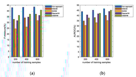
Figure 10. AUROC and F1-measure, when openness is about 0.6, for open-set multi-class recognition using different numbers of training samples on CIFAR100 open dataset: (a) F1-measure and (b) AUROC.

5. Conclusions

This paper analyzes and summarizes the reasons why the existing closed-set classifiers cannot adapt to the open-set scenario. We proposed the negative-class sample feature enhancement learning algorithm, optimized the negative-class sample feature segmentation surface based on the negative-class sample point set, and finally obtained an open-set classifier with good classification performance by establishing the paired Weibull distribution and reverse Weibull distribution of the scores from positive- and negative-class samples to the segmentation surface. In the high-openness scenario, this algorithm can effectively distinguish the known category samples from the unknown category samples and correctly classify the known category samples. Compared with other open-set classifiers, the proposed algorithm performs better in high-openness scenarios.

References

- Geng, C.; Huang, S.; Chen, S. Recent advances in open set recognition: A survey. IEEE Trans. Pattern Anal. Mach. Intell. 2020, 43, 3614–3631. [Google Scholar] [CrossRef]
- Dubuisson, B.; Masson, M. A statistical decision rule with incomplete knowledge about classes. Pattern Recognit. 1993, 26, 155–165. [Google Scholar] [CrossRef]
- Muzzolini, R.; Yang, Y.H.; Pierson, R. Classifier design with incomplete knowledge. Pattern Recognit. 1998, 31, 345–369. [Google Scholar] [CrossRef]
- Moeini, A.; Faez, K.; Moeini, H.; Safai, A.M. Open-set face recognition across look-alike faces in real-world scenarios. Image Vis. Comput. 2017, 57, 1–14. [Google Scholar] [CrossRef]
- Tax, D.M.J.; Duin, R.P.W. Support vector data description. Mach. Learn. 2004, 54, 45–66. [Google Scholar] [CrossRef]
- Schölkopf, B.; Platt, J.C.; Shawe-Taylor, J.; Smola, A.J.; Williamson, R.C. Estimating the support of a high-dimensional distribution. Neural Comput. 2001, 13, 1443–1471. [Google Scholar] [CrossRef] [PubMed]
- Cortes, C.; DeSalvo, G.; Mohri, M. Learning with rejection. In Proceedings of the International Conference on Algorithmic Learning Theory, Bari, Italy, 19–21 October 2016; Springer: Cham, Switzerland, 2016; pp. 67–82. [Google Scholar]
- Mendes Júnior, P.R.; De Souza, R.M.; Werneck, R.O.; Stein, B.V.; Pazinato, D.V.; de Almeida, W.R.; Penatti, O.A.B.; Torres, R.d.; Rocha, A. Nearest neighbors distance ratio open-set classifier. Mach. Learn. 2017, 106, 359–386. [Google Scholar] [CrossRef]
- Wen, Y.; Zhang, K.; Li, Z.; Qiao, Y. A comprehensive study on center loss for deep face recognition. Int. J. Comput. Vis. 2019, 127, 668–683. [Google Scholar] [CrossRef]
- Rocha, A.; Goldenstein, S.K. Multiclass from Binary: Expanding One-Versus-All, One-Versus-One and ECOC-Based Approaches. IEEE Trans. Neural Netw. Learn. Syst. 2017, 25, 289–302. [Google Scholar] [CrossRef]
- Jain, L.P.; Scheirer, W.J.; Boult, T.E. Multi-class open set recognition using probability of inclusion. In Proceedings of the European Conference on Computer Vision, Zurich, Switzerland, 6–12 September 2014; Springer: Cham, Switzerland, 2014; pp. 393–409. [Google Scholar]
- Xu, Y.; Liu, C. A rough margin-based one class support vector machine. Neural Comput. Appl. 2013, 22, 1077–1084. [Google Scholar] [CrossRef]
- Yang, G.; Qi, S.; Yu, T.; Wan, M.; Yang, Z.; Zhan, T.; Zhang, F.; Lai, Z. SVDTWDD Method for High Correct Recognition Rate Classifier with Appropriate Rejection Recognition Regions. IEEE Access 2020, 8, 47914–47924. [Google Scholar] [CrossRef]
- Wu, M.; Ye, J. A Small Sphere and Large Margin Approach for Novelty Detection Using Training Data with Outliers. IEEE Trans. Pattern Anal. Mach. Intell. 2009, 31, 2088–2092. [Google Scholar] [PubMed]
- Kotz, S.; Nadarajah, S. Extreme Value Distributions: Theory and Applications; Imperial College Press: London, UK, 2000. [Google Scholar]
- Scheirer, W.J.; de Rezende Rocha, A.; Parris, J.; Boult, T.E. Learning for meta-recognition. IEEE Trans. Inf. Secur. 2012, 7, 1214–1224. [Google Scholar] [CrossRef]
- Scheirer, W.J.; Rocha, A.; Micheals, R.J.; Boult, T.E. Meta-recognition: The theory and practice of recognition score analysis. IEEE Trans. Pattern Anal. Mach. Intell. 2011, 33, 1689–1695. [Google Scholar] [CrossRef] [PubMed]
- Scheirer, W.J.; Jain, L.P.; Boult, T.E. Probability models for open set recognition. IEEE Trans. Pattern Anal. Mach. Intell. 2014, 36, 2317–2324. [Google Scholar] [CrossRef] [PubMed]
- Rudd, E.M.; Jain, L.P.; Scheirer, W.J.; Boult, T.E. The extreme value machine. IEEE Trans. Pattern Anal. Mach. Intell. 2017, 40, 762–768. [Google Scholar] [CrossRef] [PubMed]
- Ding, L.; Liao, S. An Approximate Approach to Automatic Kernel Selection. IEEE Trans. Cybern. 2016, 47, 554–565. [Google Scholar] [CrossRef]
- Xu, Y. Maximum Margin of Twin Spheres Support Vector Machine for Imbalanced Data Classification. IEEE Trans. Cybern. 2016, 47, 1540–1550. [Google Scholar] [CrossRef]
- Frey, P.W.; Slate, D.J. Letter recognition using Holland-style adaptive classifiers. Mach. Learn. 1991, 6, 161–182. [Google Scholar] [CrossRef]
- Griffin, G.; Holub, A.; Perona, P. Caltech-256 Object Category Dataset. Technical Report 7694; California Institute of Technology: Pasadena, CA, USA, 2007. [Google Scholar]
- Krizhevsky, A.; Hinton, G. Learning Multiple Layers of Features from Tiny Images. Technical Report TR-2009; University of Toronto: Toronto, ON, Canada, 2009. [Google Scholar]
- Júnior, P.R.M.; Boult, T.E.; Wainer, J.; Rocha, A. Open-set support vector machines. IEEE Trans. Syst. Man Cybern. Syst. 2021, 52, 3785–3798. [Google Scholar] [CrossRef]
- Scheirer, W.J.; de Rezende Rocha, A.; Sapkota, A.; Boult, T.E. Toward open set recognition. IEEE Trans. Pattern Anal. Mach. Intell. 2012, 35, 1757–1772. [Google Scholar] [CrossRef] [PubMed]
- He, K.; Zhang, X.; Ren, S.; Sun, J. Deep Residual Learning for Image Recognition. In Proceedings of the 2016 IEEE Conference on Computer Vision and Pattern Recognition, Las Vegas, NV, USA, 27–30 June 2016; IEEE: Washington, DC, USA, 2016; pp. 770–778. [Google Scholar]
- Shi, C.; Panoutsos, G.; Luo, B.; Liu, H.; Li, B.; Lin, X. Using Multiple-Feature-Spaces-Based Deep Learning for Tool Condition Monitoring in Ultraprecision Manufacturing. IEEE Trans. Ind. Electron. 2018, 66, 3794–3803. [Google Scholar] [CrossRef]
- Scheirer, W.J.; Kumar, N.; Belhumeur, P.N.; Boult, T.E. Multi-attribute spaces: Calibration for attribute fusion and similarity search. In Proceedings of the 2012 IEEE Conference on Computer Vision and Pattern Recognition, Providence, RI, USA, 16–21 June 2012; IEEE: Washington, DC, USA, 2012; pp. 2933–2940. [Google Scholar]
Publisher’s Note: MDPI stays neutral with regard to jurisdictional claims in published maps and institutional affiliations. |
© 2022 by the authors. Licensee MDPI, Basel, Switzerland. This article is an open access article distributed under the terms and conditions of the Creative Commons Attribution (CC BY) license (https://creativecommons.org/licenses/by/4.0/).