Highly Dispersive Optical Solitons in Birefringent Fibers with Polynomial Law of Nonlinear Refractive Index by Laplace–Adomian Decomposition

Abstract

This paper is a numerical simulation of highly dispersive optical solitons in birefringent fibers with polynomial nonlinear form, which is achieved for the first time. The algorithmic approach is applied with the usage of the Laplace–Adomian decomposition scheme. Dark and bright soliton simulations are presented. The error measure has a very low count, and thus, the simulations are almost an exact replica of such solitons that analytically arise from the governing system. The suggested iterative scheme finds the solution without any discretization, linearization, or restrictive assumptions.

1. Introduction

The term highly dispersive (HD) optical soliton was conceived a couple of years ago. Later, it was studied by several authors including N. Kudryashov [1,2,3,4,5]. The two essential factors that make the propel of solitons through fibers and other waveguides possible are the self-phase modulation (SPM) and chromatic dispersion (CD). When CD runs low during soliton transmission, the balance between nonlinearity and dispersion is compromised. This would lead to a catastrophic situation. To avoid such a scenario, CD is compensated with other sources of dispersion, and they are sixth-order dispersion (6OD), fifth-order dispersion (5OD), fourth-order dispersion (4OD), third-order dispersion (3OD) and inter-modal dispersion (IMD). The inclusion of six dispersive effects secures HD solitons. This however has other detrimental effects although they are being ignored in the current paper. They are the presence of soliton radiation and the slowdown of solitons due to this shedding of energy. Pulse splitting or polarization-mode dispersion is another feature in the dynamics of optical soliton propagation that cannot be avoided. This leads to the effect of differential group delay, which cumulatively would lead to birefringence. The split-pulse dynamics in birefringent fibers is the focus of attention in the current paper. The dynamics of such soliton pulses are studied when the nonlinear form is of the polynomial type. The numerical simulations are recovered by the aid of the Laplace–Adomian decomposition method (LADM) that is a manifestation of the pre-existing Adomian decomposition approach. Dark and bright solitons are addressed in this work. The low error measure leads to an almost exact replica of solitons that have been analytically recovered in the past. The results are displayed after a recapitulation of the known analytical results.

Our work is divided in several sections. In the “Governing Equation” section, we provide a brief introduction to the model given by the highly dispersive nonlinear Schrödinger equation with cubic–quintic–septic law. We also illustrate the model by taking into account the birefringence effect. In the “Description and Application of the LADM” section, we describe the Laplace–Adomian decomposition method to be applied to approximate the solution of the highly dispersive nonlinear Schrödinger equation with polynomial law. In the “Graphical Representations” section, the results of the numerical experiment are shown in tables and graphs. Finally, in the “Conclusions” section, we summarize our findings and present our final conclusions.

2. Governing Equation

The highly dispersive nonlinear Schrödinger with polynomial nonlinear form is presented below [6,7,8,9,10,11,12,13,14,15,16]:

$$\begin{gathered} i{q}_t+i{a}_1{q}_x+a_2{q}_{xx}+i{a}_3{q}_{xxx}+a_4{q}_{xxxx}+i{a}_5{q}_{xxxxx} \\ +a_6{q}_{xxxxxx}+\left(b_1|q{|}^2+b_2|q{|}^4+b_3|q{|}^6\right)q=0. \end{gathered}$$

(1)

Here, $a_k$ ($1\le k\le 6$) and $b_l$ ($1\le l\le 3$) are real-valued constants, while $q=q\left(x,t\right)$ is a complex-valued function. $a_6$ gives 6OD, $a_5$ is associated with 5OD, $a_4$ arises from 4OD, $a_3$ stems from 3OD, $a_2$ is related to CD, and $a_1$ emerges from IMD. $x$ is the spatial variable; $q$ stands for the soliton profile; $t$ is the temporal variable; the first term signifies the temporal evolution, where $i=\sqrt{-1}$; and $b_1$, $b_2$, and $b_3$ secure the polynomial nonlinear form. Additionally, the subscript $t$ and $x$ denote distinct order temporal and spatial derivatives.

The main governing system derived from the model (1) is considered as [6]

$$\begin{gathered} i{u}_t+i{a}_1^1{u}_x+a_2^1{u}_{xx}+i{a}_3^1{u}_{xxx}+a_4^1{u}_{xxxx}+i{a}_5^1{u}_{xxxxx}+a_6^1{u}_{xxxxxx} \\ +\left(b_{11}^1|u{|}^2+b_{12}^1|v{|}^2\right)u+\left(b_{11}^2|u{|}^4+b_{12}^2|u{|}^2|v{|}^2+b_{13}^2|v{|}^4\right)u \\ +\left(b_{11}^3|u{|}^6+b_{12}^3|u{|}^4|v{|}^2+b_{13}^3|u{|}^2|v{|}^4+b_{14}^3|v{|}^6\right)u=0, \end{gathered}$$

(2)

$$\begin{gathered} i{v}_t+i{a}_1^2{v}_x+a_2^2{v}_{xx}+i{a}_3^2{v}_{xxx}+a_4^2{v}_{xxxx}+i{a}_5^2{v}_{xxxxx}+a_6^2{v}_{xxxxxx} \\ +\left(b_{21}^1|v{|}^2+b_{22}^1|u{|}^2\right)v+\left(b_{21}^2|v{|}^4+b_{22}^2|u{|}^2|v{|}^2+b_{23}^2|u{|}^4\right)v \\ +\left(b_{21}^3|v{|}^6+b_{22}^3|v{|}^4|u{|}^2+b_{23}^3|v{|}^2|u{|}^4+b_{24}^3|u{|}^6\right)v=0. \end{gathered}$$

(3)

Here, $b_{j1}^1$, $b_{j1}^2$, $b_{j1}^3$, $b_{j2}^1$, $b_{j2}^2$, $b_{j3}^2$, $b_{j2}^3$, $b_{j3}^3$, $b_{j4}^3$ ($j=1,2$), and $a_k^j$ ($1\le k\le 6$) are real-valued constants, while $v=v\left(x,t\right)$ and $u=u\left(x,t\right)$ are complex-valued functions. $b_{j1}^1$, $b_{j1}^2$, and $b_{j1}^3$ give the self-phase modulation; $u$ and $v$ stand for the soliton profiles; $b_{j2}^1$, $b_{j2}^2$, $b_{j3}^2$, $b_{j2}^3$, $b_{j3}^3$, and $b_{j4}^3$ secure the cross-phase modulation, and the first terms imply linear evolutions. $a_6^j$ gives 6OD, $a_5^j$ is associated with 5OD, $a_4^j$ arises from 4OD, $a_3^j$ stems from 3OD, $a_2^j$ is related to CD, and $a_1^j$ emerges from IMD.

It must be noted that in order to derive (2) and (3) from (1), for birefringent fibers, it is necessary to split $q\left(x,t\right)=u\left(x,t\right)+v\left(x,t\right)$, to substitute it into (1), and then to write the two components of the equation after neglecting the effects of four wave mixing.

Bright and Dark Solitons

The dark solitons with the present governing system of (2) and (3) are formulated as following [6]:

$$\{\begin{array}{l}u\left(x,t\right)=\left(A_1\tanh \left(x-{\nu }_{1}t\right)\right)e^{i\left[-{\kappa }_{1}x+{\omega }_{1}t+{\theta }_1\right]},\hfill \\ v\left(x,t\right)=\left(A_2\tanh \left(x-{\nu }_{2}t\right)\right)e^{i\left[-{\kappa }_{2}x+{\omega }_{2}t+{\theta }_2\right]},\hfill \end{array}$$

(4)

where the parameters are listed as [6]

$$A_1=\pm \sqrt{-\frac{\left(\begin{array}{c}30{\kappa }_1^4{a}_6^1-20{\kappa }_1^3{a}_5^1+600{\kappa }_1^2{a}_6^1-12{\kappa }_1^2{a}_4^1\\ -200{\kappa }_1{a}_5^1+6{\kappa }_1{a}_3^1+2a_2^1+1232a_6^1-40a_4^1\end{array}\right)}{b_{11}^1+b_{12}^1}},$$

(5)

$${\nu }_1=5a_5^1{\kappa }_1^4-6a_6^1{\kappa }_1^5-2a_2^1{\kappa }_1-3a_3^1{\kappa }_1^2+4a_4^1{\kappa }_1^3+a_1^1,$$

(6)

$$A_2=\pm \sqrt{-\frac{\left(\begin{array}{c}30{\kappa }_2^4{a}_6^2-20{\kappa }_2^3{a}_5^2+600{\kappa }_2^2{a}_6^2-12{\kappa }_2^2{a}_4^2\\ -200{\kappa }_2{a}_2^2+6{\kappa }_2{a}_3^2+2a_2^2+1232a_6^2-40a_4^2\end{array}\right)}{b_{22}^1+b_{21}^1}},$$

(7)

$${\nu }_2=5a_5^2{\kappa }_2^4-6a_6^2{\kappa }_2^5-2a_2^2{\kappa }_2-3a_3^2{\kappa }_2^2+4a_4^2{\kappa }_2^3+a_1^2,$$

(8)

with the following natural constraint:

$$\left(b_{j2}^1+b_{j1}^1\right)\left(\begin{array}{c}30{\kappa }_2^4{a}_6^2-20{\kappa }_2^3{a}_5^2+600{\kappa }_2^2{a}_6^2-12{\kappa }_2^2{a}_4^2\\ -200{\kappa }_2{a}_2^2+6{\kappa }_2{a}_3^2+2a_2^2+1232a_6^2-40a_4^2\end{array}\right)<0.$$

(9)

In the above, $A_1$ and $A_2$ are free parameters of the dark soliton, while the velocities of the two components of the dark solitons are ${\nu }_1$ and ${\nu }_2$.

The bright solitons with the strategic governing system (2) and (3) are introduced below [6]:

$$\{\begin{array}{l}u\left(x,t\right)=\left(B_1\mathrm{sech}\left(x-{\nu }_{1}t\right)\right)e^{i\left[-{\kappa }_{1}x+{\omega }_{1}t+{\theta }_1\right]},\hfill \\ v\left(x,t\right)=\left(B_2\mathrm{sech}\left(x-{\nu }_{2}t\right)\right)e^{i\left[-{\kappa }_{2}x+{\omega }_{2}t+{\theta }_2\right]},\hfill \end{array}$$

(10)

where the parameters are enumerated as

$$B_1=\pm \sqrt{\frac{\left(\begin{array}{c}30{\kappa }_1^4{a}_6^1-20{\kappa }_1^3{a}_5^1+600{\kappa }_1^2{a}_6^1-12{\kappa }_1^2{a}_4^1\\ -200{\kappa }_1{a}_5^1+6{\kappa }_1{a}_3^1+2a_2^1+1232a_6^1-40a_4^1\end{array}\right)}{b_{11}^1+b_{12}^1}},$$

(11)

$${\nu }_1=5a_5^1{\kappa }_1^4-6a_6^1{\kappa }_1^5-2a_2^1{\kappa }_1-3a_3^1{\kappa }_1^2+4a_4^1{\kappa }_1^3+a_1^1,$$

(12)

$$B_2=\pm \sqrt{\frac{\left(\begin{array}{c}30{\kappa }_2^4{a}_6^2-20{\kappa }_2^3{a}_5^2+600{\kappa }_2^2{a}_6^2-12{\kappa }_2^2{a}_4^2\\ -200{\kappa }_2{a}_2^2+6{\kappa }_2{a}_3^2+2a_2^2+1232a_6^2-40a_4^2\end{array}\right)}{b_{22}^1+b_{21}^1}},$$

(13)

$${\nu }_2=5a_5^2{\kappa }_2^4-6a_6^2{\kappa }_2^5-2a_2^2{\kappa }_2-3a_3^2{\kappa }_2^2+4a_4^2{\kappa }_2^3+a_1^2,$$

(14)

with the following natural constraint:

$$\left(b_{j2}^1+b_{j1}^1\right)\left(\begin{array}{c}30{\kappa }_2^4{a}_6^2-20{\kappa }_2^3{a}_5^2+600{\kappa }_2^2{a}_6^2-12{\kappa }_2^2{a}_4^2\\ -200{\kappa }_2{a}_2^2+6{\kappa }_2{a}_3^2+2a_2^2+1232a_6^2-40a_4^2\end{array}\right)>0.$$

(15)

In this context, the parameters $B_1$ and $B_2$ are the amplitudes of the two components of bright solitons that travel with velocities ${\nu }_1$ and ${\nu }_2$, respectively.

3. Description and Application of the LADM

The integration scheme is derived from the decomposition algorithm that has been reported in [17] by the aid of Laplace transform [18]. The solution of a governing model is structured as the local truncation of a convergent series of functions [19].

To address this scheme, the governing system (2) and (3) is presented below:

$$\begin{gathered} u_t=-a_1^1{u}_x+i{a}_2^1{u}_{xx}-a_3^1{u}_{xxx}+i{a}_4^1{u}_{xxxx} \\ -a_5^1{u}_{xxxxx}+i{a}_6^1{u}_{xxxxxx}+i{N}_1\left(u,v\right), \end{gathered}$$

(16)

$$\begin{gathered} v_t=-a_1^2{v}_x+i{a}_2^2{v}_{xx}-a_3^2{v}_{xxx}+i{a}_4^2{v}_{xxxx} \\ -a_5^2{v}_{xxxxx}+i{a}_6^2{v}_{xxxxxx}+i{N}_2\left(u,v\right). \end{gathered}$$

(17)

Equations (16) and (17) are also formulated as

$$D_{t}u=i{N}_1\left(u,v\right)+{\displaystyle \sum }_{k=1}^3\left(i{a}_{2k}^1{D}_x^{2k}-a_{2k-1}^1{D}_x^{2k-1}\right)u,$$

(18)

$$D_{t}u=i{N}_2\left(u,v\right)+{\displaystyle \sum _{k=1}^3\left(i{a}_{2k}^2{D}_x^{2k}-a_{2k-1}^2{D}_x^{2k-1}\right)v}$$

(19)

by virtue of initial conditions $v\left(x,0\right)=g\left(x\right)$ and $u\left(x,0\right)=f\left(x\right)$. Here, $N_j$ are differential operators containing all nonlinear terms, $D_x^k$ stands for a partial derivative of order $k$ in terms of the independent variable $x$, and $D_t$ stands for first-order derivative in terms of the independent variable $t$. Thus, the operators $N_j$ are presented below:

$$\begin{gathered} N_2\left(u,v\right)=\left(b_{21}^2|v{|}^4+b_{22}^2|u{|}^2|v{|}^2+b_{23}^2|u{|}^4\right)v+\left(b_{21}^1|v{|}^2+b_{22}^1|u{|}^2\right)v \\ +\left(b_{21}^3|v{|}^6+b_{22}^3|v{|}^4|u{|}^2+b_{23}^3|v{|}^2|u{|}^4+b_{24}^3|u{|}^6\right)v, \end{gathered}$$

(20)

$$\begin{gathered} N_1\left(u,v\right)=\left(b_{11}^2|u{|}^4+b_{12}^2|u{|}^2|v{|}^2+b_{13}^2|v{|}^4\right)u+\left(b_{11}^1|u{|}^2+b_{12}^1|v{|}^2\right)u \\ +\left(b_{11}^3|u{|}^6+b_{12}^3|u{|}^4|v{|}^2+b_{13}^3|u{|}^2|v{|}^4+b_{14}^3|v{|}^6\right)u. \end{gathered}$$

(21)

Using the Laplace transform in the system with (18) and (19) along with the initial conditions, one secures

$$v\left(x,s\right)=\frac{1}{s}ℒ\left\{{\displaystyle \sum }_{k=1}^3\left(i{a}_{2k}^2{D}_x^{2k}-a_{2k-1}^2{D}_x^{2k-1}\right)v+i{N}_2\left(u,v\right)\right\}+\frac{g\left(x\right)}{s},$$

(22)

$$u\left(x,s\right)=\frac{1}{s}ℒ\left\{{\displaystyle \sum }_{k=1}^3\left(i{a}_{2k}^1{D}_x^{2k}-a_{2k-1}^1{D}_x^{2k-1}\right)u+i{N}_1\left(u,v\right)\right\}+\frac{f\left(x\right)}{s}.$$

(23)

By the aid of the conventional inverse Laplace transform ${ℒ}^{-1}$, we arrive at the following:

$$v\left(x,t\right)={ℒ}^{-1}\left[\frac{1}{s}ℒ\left\{{\displaystyle \sum }_{k=1}^3\left(i{a}_{2k}^2{D}_x^{2k}-a_{2k-1}^2{D}_x^{2k-1}\right)v+i{N}_2\left(u,v\right)\right\}\right]+v\left(x,0\right),$$

(24)

$$u\left(x,t\right)={ℒ}^{-1}\left[\frac{1}{s}ℒ\left\{{\displaystyle \sum _{k=1}^3\left(i{a}_{2k}^1{D}_x^{2k}-a_{2k-1}^1{D}_x^{2k-1}\right)u+i{N}_1\left(u,v\right)}\right\}\right]+u\left(x,0\right).$$

(25)

Now, the solution functions $v$ and $u$ in the Adomian decomposition algorithm are extracted as

$$v\left(x,t\right)={\displaystyle \sum }_{n=0}^{\infty }{v}_n\left(x,t\right),\hspace{1em}\hspace{1em}u\left(x,t\right)={\displaystyle \sum }_{n=0}^{\infty }{u}_n\left(x,t\right).$$

(26)

Additionally, the nonlinear terms in Equations (20) and (21) are decomposed in Adomian polynomials [17,18,19] as

$$\begin{gathered} N_2\left(u,v\right)=\left(b_{21}^2|v{|}^4+b_{22}^2|u{|}^2|v{|}^2+b_{23}^2|u{|}^4\right)v+\left(b_{21}^1|v{|}^2+b_{22}^1|u{|}^2\right)v \\ +\left(b_{21}^3|v{|}^6+b_{22}^3|v{|}^4|u{|}^2+b_{23}^3|v{|}^2|u{|}^4+b_{24}^3|u{|}^6\right)v \\ ={\displaystyle \sum }_{n=0}^{\infty }{B}_n\left(u_0,\dots ,u_n;v_0,\dots ,v_n\right), \end{gathered}$$

(27)

$$\begin{gathered} N_1\left(u,v\right)=\left(b_{11}^2|u{|}^4+b_{12}^2|u{|}^2|v{|}^2+b_{13}^2|v{|}^4\right)u+\left(b_{11}^1|u{|}^2+b_{12}^1|v{|}^2\right)u \\ +\left(b_{11}^3|u{|}^6+b_{12}^3|u{|}^4|v{|}^2+b_{13}^3|u{|}^2|v{|}^4+b_{14}^3|v{|}^6\right)u \\ ={\displaystyle \sum }_{n=0}^{\infty }{A}_n\left(u_0,\dots ,u_n;v_0,\dots ,v_n\right), \end{gathered}$$

(28)

where $A_n$ and $B_n$ are enumerated as follows [20]:

$$\{\begin{array}{l}{B}_0=\left(b_{21}^1|v_0{|}^2+b_{22}^1|u_0{|}^2\right)v_0+\left(b_{21}^2|v_0{|}^4+b_{22}^2|u_0{|}^2|v_0{|}^2+b_{23}^2|u_0{|}^4\right)v_0\hfill \\ +\left(b_{21}^3|v_0{|}^6+b_{22}^3|v_0{|}^4|u_0{|}^2+b_{23}^3|v_0{|}^2|u_0{|}^4+b_{24}^3|u_0{|}^6\right)v_0,\hfill \\ B_n=\frac{1}{n}{\displaystyle {\displaystyle \sum }_{k=0}^{n-1}}\left(k+1\right)\left(u_{k+1}\frac{\partial }{\partial u_k}{B}_{n-1}+v_{k+1}\frac{\partial }{\partial v_k}{B}_{n-1}\right), n\ge 1,\hfill \end{array}$$

(29)

$$\{\begin{array}{l}{A}_0=\left(b_{11}^1|u_0{|}^2+b_{12}^1|v_0{|}^2\right)u_0+\left(b_{11}^2|u_0{|}^4+b_{12}^2|u_0{|}^2|v_0{|}^2+b_{13}^2|v_0{|}^4\right)u_0\hfill \\ +\left(b_{11}^3|u_0{|}^6+b_{12}^3|u_0{|}^4|v_0{|}^2+b_{13}^3|u_0{|}^2|v_0{|}^4+b_{14}^3|v_0{|}^6\right)u_0,\hfill \\ A_n=\frac{1}{n}{\displaystyle {\displaystyle \sum }_{k=0}^{n-1}}\left(k+1\right)\left(u_{k+1}\frac{\partial }{\partial u_k}{A}_{n-1}+v_{k+1}\frac{\partial }{\partial v_k}{A}_{n-1}\right), n\ge 1.\hfill \end{array}$$

(30)

Plugging (26)–(28) into (24) and (25) yields the solution functions:

$${\displaystyle \sum }_{n=0}^{\infty }{v}_n={ℒ}^{-1}\left[\frac{1}{s}ℒ\left\{{\displaystyle \sum }_{k=1}^3\left(i{a}_{2k}^2{D}_x^{2k}-a_{2k-1}^2{D}_x^{2k-1}\right){\displaystyle \sum }_{n=0}^{\infty }{v}_n+i{\displaystyle \sum }_{n=0}^{\infty }{B}_n\right\}\right]+v\left(x,0\right),$$

(31)

$${\displaystyle \sum }_{n=0}^{\infty }{u}_n={ℒ}^{-1}\left[\frac{1}{s}ℒ\left\{{\displaystyle \sum }_{k=1}^3\left(i{a}_{2k}^1{D}_x^{2k}-a_{2k-1}^1{D}_x^{2k-1}\right){\displaystyle \sum }_{n=0}^{\infty }{u}_n+i{\displaystyle \sum }_{n=0}^{\infty }{A}_n\right\}\right]+u\left(x,0\right).$$

(32)

Therefore, the $v_n$ and $u_n$ components for the system with (16) and (17) are yielded by the following algorithm:

$$\{\begin{array}{l}{u}_{n+1}\left(x,t\right)={ℒ}^{-1}\left[\frac{1}{s}ℒ\left\{{\displaystyle {\displaystyle \sum }_{k=1}^3}\left(i{a}_{2k}^1{D}_x^{2k}-a_{2k-1}^1{D}_x^{2k-1}\right)u_n+i{A}_n\right\}\right], n\ge 0,\hfill \\ u_0\left(x,t\right)=u\left(x,0\right)=f\left(x\right),\hfill \end{array}$$

(33)

$$\{\begin{array}{l}{v}_{n+1}\left(x,t\right)={ℒ}^{-1}\left[\frac{1}{s}ℒ\left\{{\displaystyle {\displaystyle \sum }_{k=1}^3}\left(i{a}_{2k}^2{D}_x^{2k}-a_{2k-1}^2{D}_x^{2k-1}\right)v_n+i{B}_n\right\}\right], n\ge 0,\hfill \\ v_0\left(x,t\right)=v\left(x,0\right)=g\left(x\right).\hfill \end{array}$$

(34)

Finally, adding the components $u_n\left(x,t\right)$ and $v_n\left(x,t\right)$ along with the solution functions in (26), an approximation for the system with (16) and (17) is obtained.

Convergence of the Proposed Method

The following theorem provides a necessary condition for the convergence of the proposed technique. The results are standard and can be seen in [21].

Theorem 1.

Let $N$ be an operator from a Hilbert Space $H$ into $H$, and let $u$ be an exact solution of Equation (1). ${{\displaystyle \sum }}_{j=0}^{\infty }{u}_j$ converges to the exact solution $u$, if there exists $\beta$, $0\le \beta <1$, such that $\left|\left|u_{k+1}\left|\left|\le \beta \right|\right|u_k\right|\right|$, for every $k\ge 0$.

Proof of Theorem 1.

We have

$$\begin{gathered} S_0=0, \\ {S}_1=S_0+u_1=u_1, \\ {S}_2=S_1+u_2=u_1+u_2, \\ ⋮ \\ {S}_n=S_{n-1}+u_n=u_1+u_2+\dots +u_n, \end{gathered}$$

and we show that $\left\{S_n\right\}$ is a Cauchy sequence in a Hilbert Space $H$. Now, for

$$\left|\left|S_{n+1}-S_n\left||=|\right|u_{n+1}\left|\left|\le \beta \right|\right|u_n\right|\right|\le {\beta }^2\left|\left|u_{n-1}\right|\right|\le \dots \le {\beta }^{n+1}\left|\left|u_0\right|\right|,$$

for every $n,m\in \mathbb{N}$, $n\ge m$, we have

$$\begin{array}{ll}\left|\left|S_n-S_m\right|\right|\hfill & =\left|\left|\left(S_n-S_{n-1}\right)+\left(S_{n-1}-S_{n-2}\right)+\cdots +\left(S_{m+1}-S_m\right)\right|\right|\hfill \\ & \le \left|\left|S_n-S_{n-1}\left||+|\right|S_{n-1}-S_{n-2}\left|\left|+\cdots +\right|\right|S_{m+1}-S_m\right|\right|\hfill \\ & \le {\beta }^n\left|\left|u_0\right|\right|+{\beta }^{n-1}\left|\left|u_0\right|\right|+\cdots +{\beta }^{m+1}\left|\left|u_0\right|\right|\hfill \\ & \le \left({\beta }^{m+1}+{\beta }^{m+2}+\cdots \right)\left|\left|u_0\right|\right|=\frac{{\beta }^{m+1}}{1-\beta }\left|\left|u_0\right|\right|\hfill \end{array}$$

From the previous inequality, we have

$$\left|\left|S_n-S_m\right|\right|\to 0, as n\to \infty ,m\to \infty .$$

Hence, $\left\{S_n\right\}$ is the Cauchy sequence in the Hilbert space $H$; therefore, it has a limit $u\in H$, which is the exact solution of Equation (1), namely

$$u=\underset{n\to \infty }{\lim }{S}_n.$$

Now, we have the following theorem, of which the proof is a direct consequence of Theorem 1. □

Theorem 2.

Assume that $u$ is the exact solution of Equation (1). Let $\left\{S_N\right\}$ be the sequence of the approximate series solutions defined by Equation (26). Then, it holds for every $t\ge 0$.

$$\underset{a\le x,y\le b}{\max }|u\left(x,y,t\right)-{\displaystyle \sum }_{j=0}^N{u}_j\left(x,y,t\right)|\le \frac{{\beta }^{m+1}}{1-\beta }\left|\left|u_0\right|\right|.$$

From this analysis, it is evident that the Adomian decomposition method combined with the Laplace transform requires less effort in comparison with the traditional Adomian decomposition method. This method considerably decreases the number of calculations. In addition, the Adomian decomposition procedure is easily established without requiring the problem to be linearized.

4. Graphical Representations

In this section, we solve some numerical examples, and we also present the results obtained graphically as well as the absolute error committed by the LADM approximation. Additional references to the recent application of LADM to a similar mathematical model can be seen in [22,23,24].

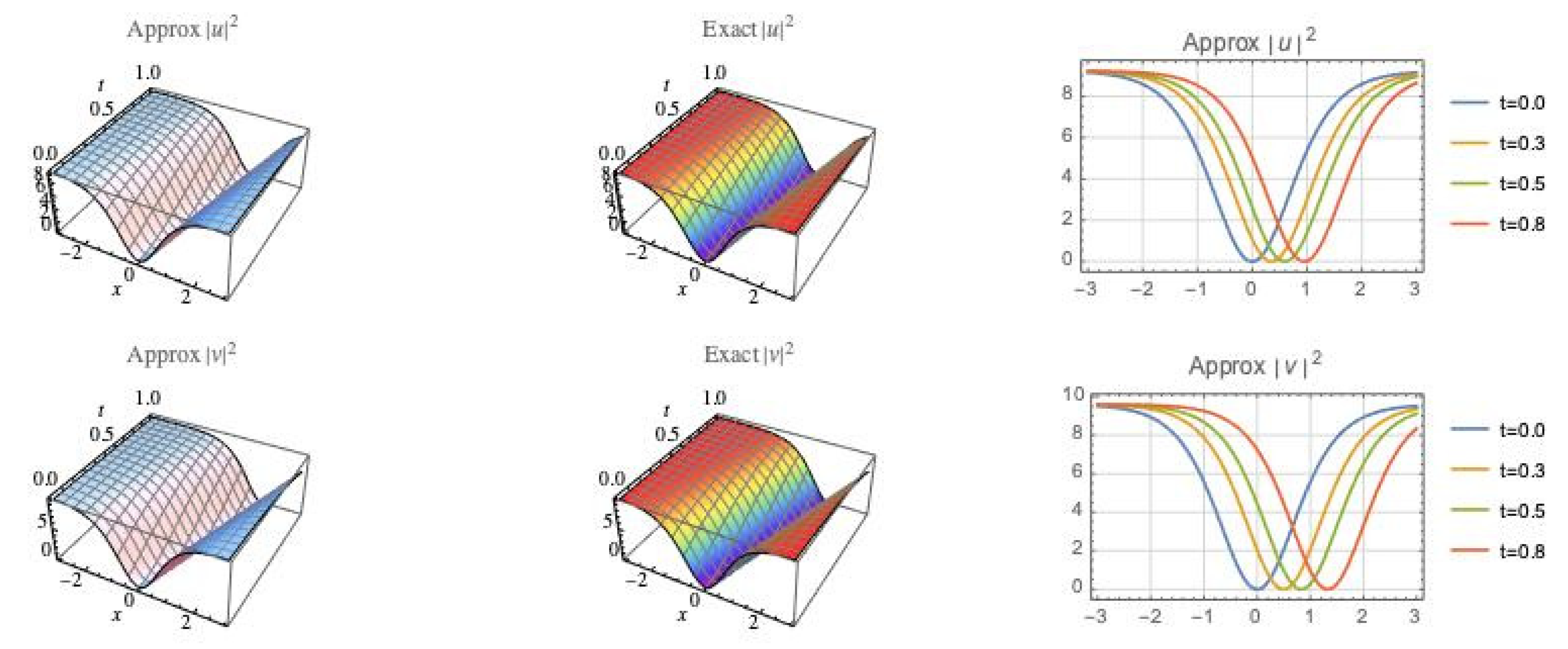
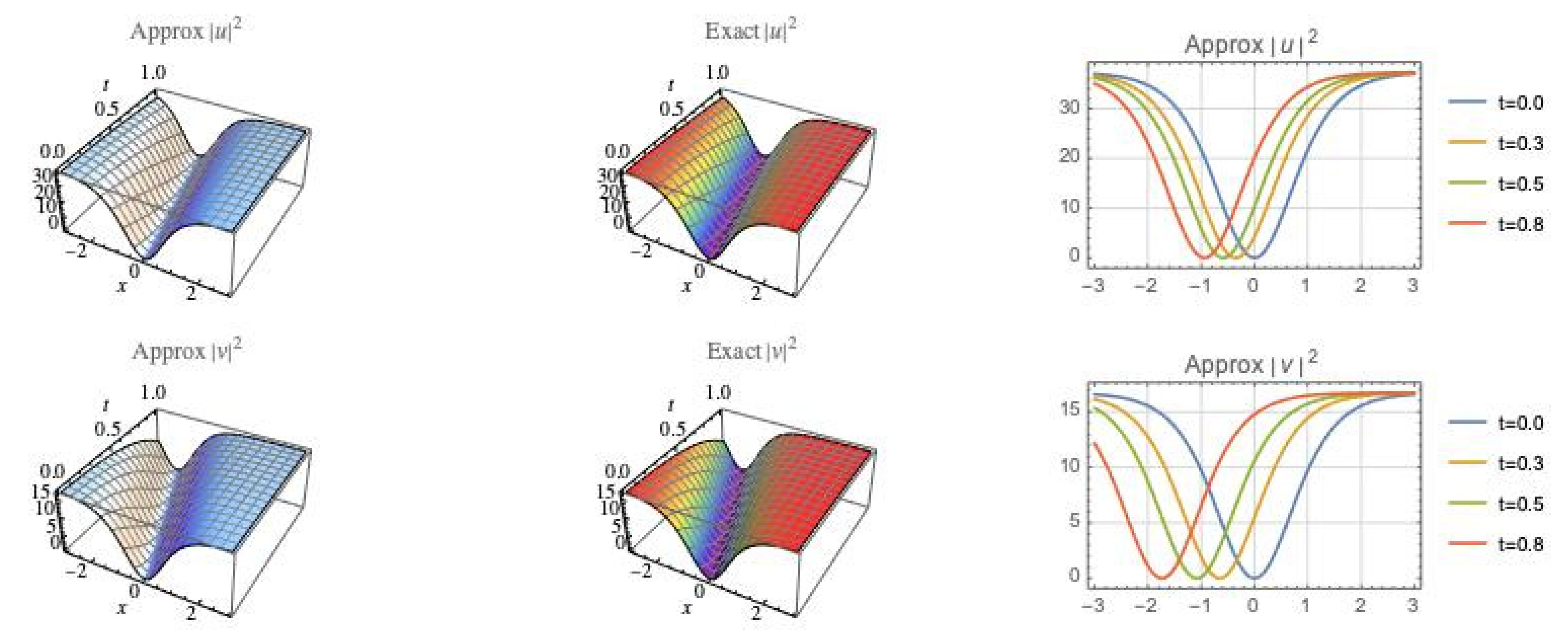
4.1. Dark Soliton Simulation

To display the dark soliton numerical simulation for the governing system (2) and (3), we consider the following coefficients:

Case A: Let us consider the following:

$$\{\begin{array}{l}{a}_1^1=1.34, a_2^1=1.5, a_3^1=-3.2, a_4^1=-2.1, a_5^1=5.2, a_6^1=0.21, \\ b_1^1=6.2, b_{11}^2=3.3, b_{12}^2=0.11,a_1^2=0.67, a_2^2=3.1, a_3^2=-0.3,\\ a_4^2=1.1, a_5^2=-5.9, a_6^2=0.33, b_2^1=4.6, b_{21}^2=2.2, b_{22}^2=3.7.\end{array}$$

(35)

Together with the initial conditions, we obtain the following:

$$f\left(x\right)=3.04\tanh \left(x\right)e^{i\left[-0.22x+0.76\right]},$$

$$g\left(x\right)=2.91\tanh \left(x\right)e^{i\left[1.13x-2.34\right]}.$$

The 2D and 3D illustrations for $|v{|}^2$ and $|u{|}^2$ for this case are shown in Figure 1. In Table 1, we show the absolute error committed in the numerical simulation of the present case for different values of the $\left(x,t\right)$ pair and for $N=15$.

Figure 1. (Above) Three-dimensional illustrations of the numerical simulation and exact solution, and two-dimensional illustration of the approximation of $|u{|}^2$; (Below) three-dimensional illustrations of the numerical simulation and exact solution, and two-dimensional illustration of the approximation of $|v{|}^2$ for Case A.

Table 1. Case A: Absolute error for different values of $\left(x,t\right)$ considering $N=15$ steps.

$\left(\mathit{t},\mathit{x}\right)$	$-2.0$	$-1.0$	$0$	$1.0$	$2.0$
$0.1$	$4.7\times {10}^{-8}$	$3.5\times {10}^{-8}$	$2.3\times {10}^{-9}$	$3.9\times {10}^{-8}$	$5.2\times {10}^{-8}$
$0.3$	$5.0\times {10}^{-7}$	$4.6\times {10}^{-7}$	$3.7\times {10}^{-8}$	$4.9\times {10}^{-7}$	$6.1\times {10}^{-7}$
$0.5$	$5.2\times {10}^{-7}$	$5.6\times {10}^{-7}$	$4.9\times {10}^{-7}$	$5.8\times {10}^{-7}$	$7.0\times {10}^{-6}$
$0.8$	$6.1\times {10}^{-5}$	$4.8\times {10}^{-5}$	$5.5\times {10}^{-7}$	$4.3\times {10}^{-5}$	$6.9\times {10}^{-5}$

Case B: Let us consider the following:

$$\{\begin{array}{c}{a}_1^1=0.33, a_2^1=0.89, a_3^1=-1.4, a_4^1=0.9, a_5^1=1.1, a_6^1=0.59, \\ b_1^1=2.2, b_{11}^2=1.23, b_{12}^2=0.5,a_1^2=8.1, a_2^2=0.36, a_3^2=1.1,\\ a_4^2=-0.27, a_5^2=3.22, a_6^2=1.06, b_2^1=2.8, b_{21}^2=0.66, b_{22}^2=2.3.\end{array}$$

(36)

By the aid of the initial conditions, we obtain the following:

$$g\left(x\right)=4.09\tanh \left(x\right)e^{i\left[2.09x+0.95\right]},$$

$$f\left(x\right)=6.11\tanh \left(x\right)e^{i\left[5.5x+1.23\right]}.$$

The 2D and 3D illustrations for $|v{|}^2$ and $|u{|}^2$ for this case are shown in Figure 2. In Table 2, we show the absolute error committed in the numerical simulation of the present case for different values of the $\left(x,t\right)$ pair and for $N=15$.

Figure 2. (Above) Three-dimensional illustrations of the numerical simulation and exact solution, and two-dimensional illustration of the approximation of $|u{|}^2$; (Below) three-dimensional illustrations of the numerical simulation and exact solution, and two-dimensional illustration of the approximation of $|v{|}^2$ for Case B.

Table 2. Case B: Absolute error for different values of $\left(x,t\right)$ considering $N=15$ steps.

$\left(\mathit{t},\mathit{x}\right)$	$-2.0$	$-1.0$	$0$	$1.0$	$2.0$
$0.1$	$3.2\times {10}^{-8}$	$3.0\times {10}^{-8}$	$2.1\times {10}^{-9}$	$3.3\times {10}^{-8}$	$3.8\times {10}^{-8}$
$0.3$	$6.1\times {10}^{-7}$	$5.1\times {10}^{-7}$	$3.4\times {10}^{-8}$	$5.6\times {10}^{-7}$	$6.7\times {10}^{-7}$
$0.5$	$6.8\times {10}^{-7}$	$6.0\times {10}^{-7}$	$2.9\times {10}^{-7}$	$6.2\times {10}^{-7}$	$6.9\times {10}^{-6}$
$0.8$	$7.2\times {10}^{-5}$	$6.4\times {10}^{-5}$	$3.5\times {10}^{-7}$	$6.6\times {10}^{-5}$	$8.0\times {10}^{-5}$

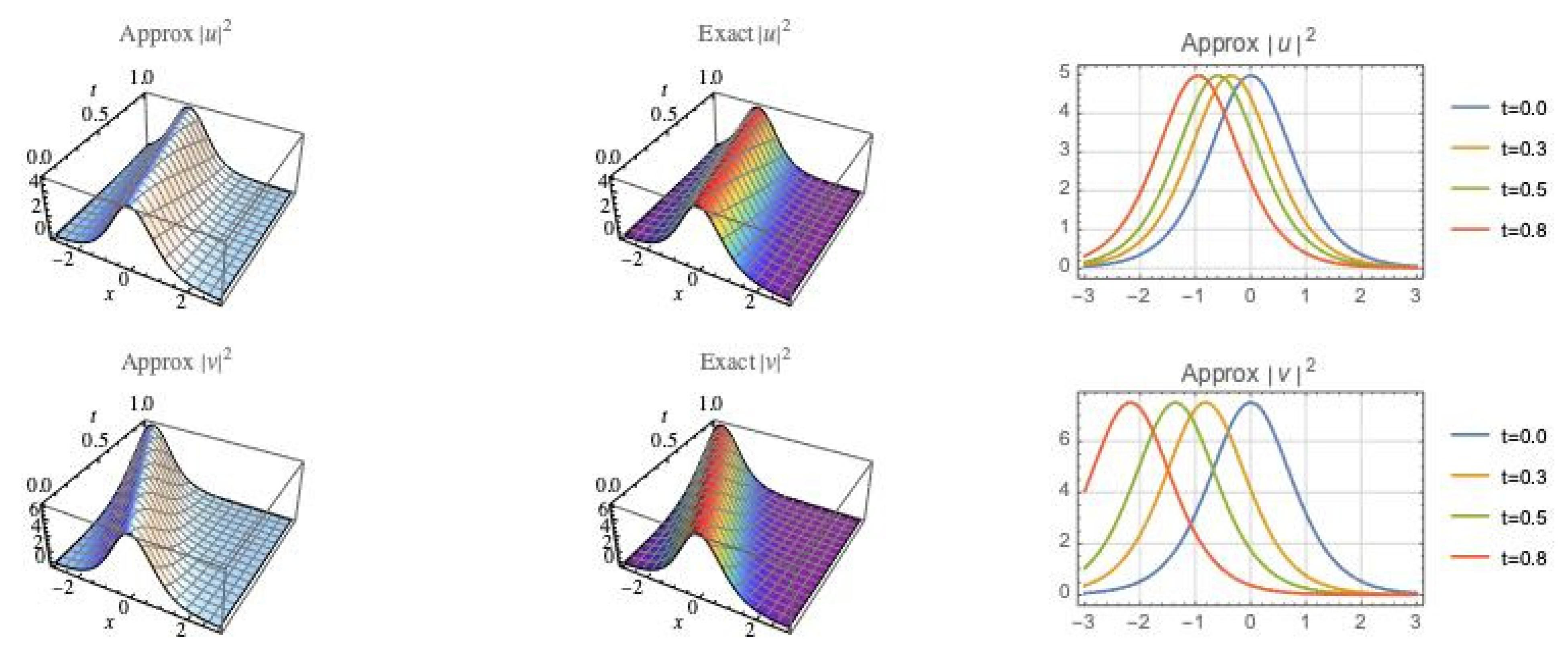
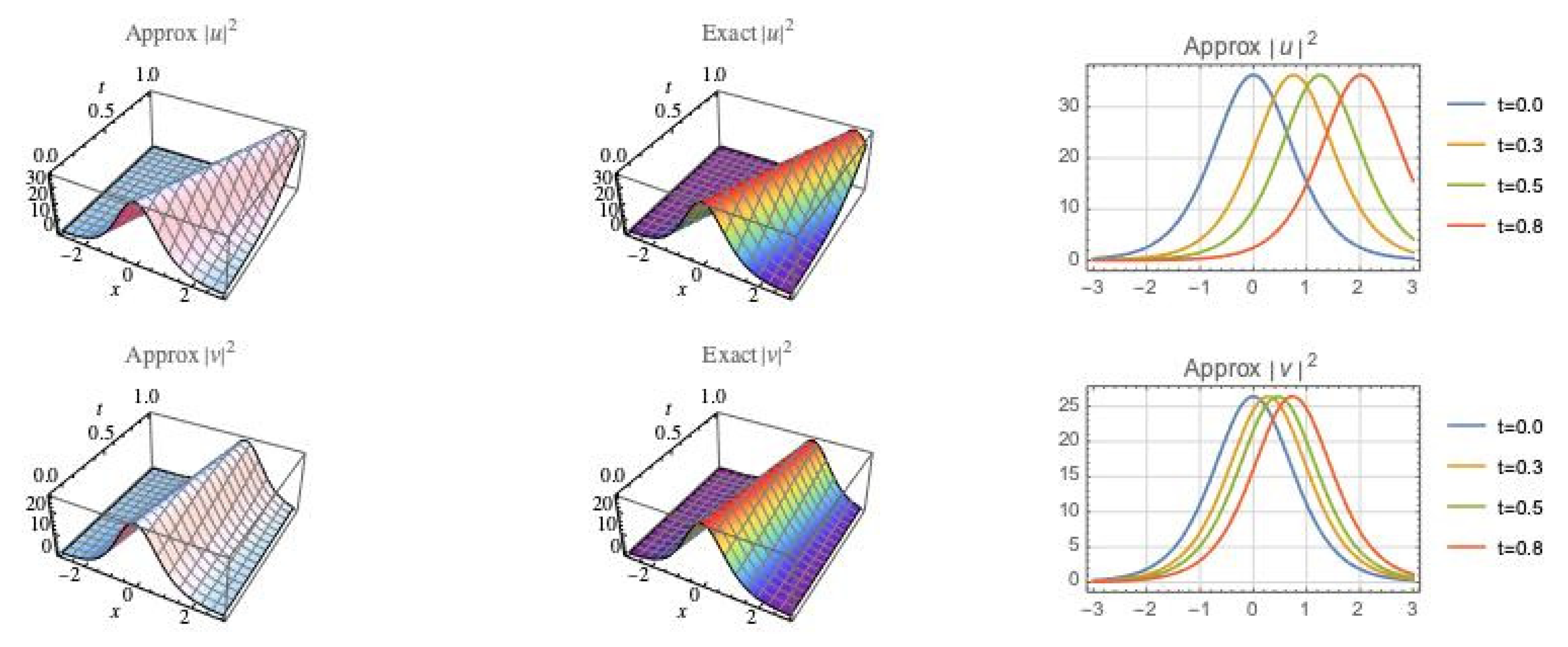
4.2. Bright Soliton Simulation

To depict the bright soliton numerical simulation for the governing system (2) and (3), we consider the following coefficients:

Case C: Let us consider the following:

$$\{\begin{array}{c}{a}_1^1=0.01, a_2^1=1.23, a_3^1=0.53, a_4^1=0.11, a_5^1=0.97, a_6^1=1.6, \\ b_1^1=3.6, b_{11}^2=1.11, b_{12}^2=2.6,a_1^2=3.01, a_2^2=0.12, a_3^2=3.6,\\ a_4^2=-4.7, a_5^2=-2.01, a_6^2=0.2, b_2^1=0.3, b_{21}^2=6.1, b_{22}^2=2.11.\end{array}$$

(37)

With the help of the initial conditions, we obtain the following:

$$g\left(x\right)=2.74\mathrm{sech}\left(x\right)e^{i\left[8.34x-0.35\right]},$$

$$f\left(x\right)=2.23\mathrm{sech}\left(x\right)e^{i\left[-3.09x-1.01\right]}.$$

The 2D and 3D illustrations for $|v{|}^2$ and $|u{|}^2$ for this case are shown in Figure 3. In Table 3, we show the absolute error committed in the numerical simulation of the present case for different values of the $\left(x,t\right)$ pair and for $N=15$.

Figure 3. (Above) Three-dimensional illustrations of the numerical simulation and exact solution, and two-dimensional illustration of the approximation of $|u{|}^2$; (Below) three-dimensional illustrations of the numerical simulation and exact solution, and two-dimensional illustration of the approximation of $|v{|}^2$ for Case C.

Table 3. Case C: Absolute error for different values of $\left(x,t\right)$ considering $N=15$ steps.

$\left(\mathit{t},\mathit{x}\right)$	$-2.0$	$-1.0$	$0$	$1.0$	$2.0$
$0.1$	$4.5\times {10}^{-8}$	$3.7\times {10}^{-8}$	$1.8\times {10}^{-9}$	$3.2\times {10}^{-8}$	$4.9\times {10}^{-8}$
$0.3$	$4.4\times {10}^{-7}$	$4.7\times {10}^{-7}$	$2.3\times {10}^{-9}$	$4.6\times {10}^{-7}$	$4.0\times {10}^{-7}$
$0.5$	$8.8\times {10}^{-7}$	$5.7\times {10}^{-7}$	$3.3\times {10}^{-8}$	$5.2\times {10}^{-7}$	$8.3\times {10}^{-6}$
$0.8$	$7.2\times {10}^{-5}$	$3.4\times {10}^{-5}$	$7.5\times {10}^{-8}$	$2.9\times {10}^{-5}$	$7.0\times {10}^{-5}$

Case D: Let us consider the following:

$$\{\begin{array}{c}{a}_1^1=9.0, a_2^1=4.2, a_3^1=0.33, a_4^1=0.31,a_5^1=0.08,a_6^1=0.03,\\ b_1^1=5.08, b_{11}^2=4.1, b_{12}^2=-9.2,a_1^2=1.16,a_2^2=0.4,a_3^2=-9.0,\\ a_4^2=-2.03,a_5^2=0.1, a_6^2=0.21,b_2^1=2.1, b_{21}^2=0.7,b_{22}^2=0.33.\end{array}$$

(38)

By virtue of the initial conditions, we obtain the following:

$$f\left(x\right)=6.02\mathrm{sech}\left(x\right)e^{i\left[-0.57x-36.01\right]},$$

$$g\left(x\right)=5.74\mathrm{sech}\left(x\right)e^{i\left[11.6x+3.08\right]}.$$

The 2D and 3D illustrations for $|v{|}^2$ and $|u{|}^2$ for this case are shown in Figure 4. In Table 4, we show the absolute error committed in the numerical simulation of the present case for different values of the $\left(x,t\right)$ pair and for $N=15$.

Figure 4. (Above) Three-dimensional illustrations of the numerical simulation and exact solution, and two-dimensional illustration of the approximation of $|u{|}^2$; (Below) three-dimensional illustrations of the numerical simulation and exact solution, and two-dimensional illustration of the approximation of $|v{|}^2$ for Case D.

Table 4. Case D: Absolute error for different values of $\left(x,t\right)$ considering $N=15$ steps.

$\left(\mathit{t},\mathit{x}\right)$	$-2.0$	$-1.0$	$0$	$1.0$	$2.0$
$0.1$	$7.2\times {10}^{-8}$	$4.4\times {10}^{-8}$	$5.2\times {10}^{-9}$	$4.2\times {10}^{-8}$	$6.9\times {10}^{-8}$
$0.3$	$6.3\times {10}^{-7}$	$4.7\times {10}^{-7}$	$6.3\times {10}^{-9}$	$4.6\times {10}^{-7}$	$5.3\times {10}^{-7}$
$0.5$	$7.8\times {10}^{-7}$	$5.9\times {10}^{-7}$	$7.7\times {10}^{-8}$	$5.5\times {10}^{-7}$	$8.0\times {10}^{-6}$
$0.8$	$8.3\times {10}^{-5}$	$2.4\times {10}^{-5}$	$9.0\times {10}^{-7}$	$3.1\times {10}^{-5}$	$9.1\times {10}^{-5}$

From the physics perspective, the surface plots of HD bright and dark solitons are accurate representations of the actual pulses that travel down an optical fiber based on the studied model. The error measure is impressive and acceptable as computed. These pulses are computed in such a way that the radiation component is completely avoided so that the core soliton regime is under focus, both for bright and dark solitons. Another source to receive a visual effect to the model would be an oscilloscope, which is outside the scope of the current work since this paper focuses on a specific numerical scheme, namely the application of LADM to handle HD solitons with polynomial law of nonlinear refractive index change.

5. Conclusions

This paper is an exhibit of numerical simulations for dark and bright HD solitons with polynomial nonlinear form. The LADM scheme has made this display possible. Dark and bright soliton surface plots are included with an error measure that is impressively small. The results are thus a step towards the final goal that is to address the model in dispersion-flattened fibers. The immediate next thought, however, is the study of HD solitons with non-local nonlinearity.

The current results are going to be pretty helpful with its implementation in a photonics lab when the experimental research is conducted to take a look at the eye diagrams without the soliton radiation. The results of this paper would therefore provide a forefront view of the bright and dark HD solitons. Thus, apart from physicists and mathematicians, the results would reach the desk of electrical engineers, whose successful observations on an oscilloscope would be closer to reality. These observations would be just before rubber meets the road.

Other areas of expansion would be to address the model with the inclusion of the effect of soliton radiation. With HD solitons, soliton radiation is unavoidable and that would unavoidably be quite pronounced. Therefore, it is imperative to include its effect and to study the model with its presence. This would require the usage of beyond all-order asymptotics and/or the theory of unfoldings to quantify the radiation effect followed by its numerical implementation. Such studies will be taken up with time, and the results will be disseminated thereafter.

References

- Kudryashov, N.A. Highly dispersive optical solitons of an equation with arbitrary refractive index. Regul. Chaotic Dyn. 2020, 25, 537–543. [Google Scholar] [CrossRef]
- Kudryashov, N.A. Highly dispersive optical solitons of equation with various polynomial nonlinearity law. Chaos Soliton Fract. 2020, 140, 110202. [Google Scholar] [CrossRef]
- Kudryashov, N.A. Highly dispersive optical solitons of the generalized nonlinear eighth-order Schrödinger equation. Optik 2020, 206, 164335. [Google Scholar] [CrossRef]
- Kudryashov, N.A. Method for finding highly dispersive optical solitons of nonlinear differential equations. Optik 2020, 206, 163550. [Google Scholar] [CrossRef]
- Kudryashov, N.A. Highly dispersive solitary wave solutions of perturbed nonlinear Schrödinger equations. Appl. Math. Comput. 2020, 371, 124972. [Google Scholar] [CrossRef]
- Yildirim, Y.; Biswas, A.; Ekici, M.; Zayed, E.M.E.; Khan, S.; Moraru, L.; Alzahrani, A.K.; Belic, M.R. Highly dispersive optical solitons in birefringent fibers with four forms of nonlinear refractive index by three prolific integration schemes. Optik 2020, 220, 165039. [Google Scholar] [CrossRef]
- Wazwaz, A.M. Bright and dark optical solitons for (3+1)-dimensional Schrödinger equation with cubic–quintic-septic nonlinearities. Optik 2021, 225, 165752. [Google Scholar] [CrossRef]
- Wazwaz, A.M.; Khuri, S.A. Two (3+1)-dimensional Schrödinger equations with cubic–quintic–septic nonlinearities: Bright and dark optical solitons. Optik 2021, 235, 166646. [Google Scholar] [CrossRef]
- Mirzazadeh, M.; Akinyemi, L.; Senol, M.; Hosseini, K. A variety of solitons to the sixth-order dispersive (3+1)-dimensional nonlinear time-fractional Schrödinger equation with cubic-quintic-septic nonlinearities. Optik 2021, 241, 166318. [Google Scholar] [CrossRef]
- Kerbouche, M.; Hamaizi, Y.; El-Akrmi, A.; Triki, H. Solitary wave solutions of the cubic-quintic-septic nonlinear Schrödinger equation in fiber Bragg gratings. Optik 2016, 127, 9562–9570. [Google Scholar] [CrossRef]
- Rabie, W.B.; Ahmed, H.M. Optical solitons for multiple-core couplers with polynomial law of nonlinearity using the modified extended direct algebraic method. Optik 2022, 258, 168848. [Google Scholar] [CrossRef]
- Rabie, W.B.; Ahmed, H.M. Cubic-quartic optical solitons and other solutions for twin-core couplers with polynomial law of nonlinearity using the extended F-expansion method. Optik 2022, 253, 168575. [Google Scholar] [CrossRef]
- Wang, M.-Y. Optical solitons with perturbed complex Ginzburg–Landau equation in kerr and cubic–quintic–septic nonlinearity. Results Phys. 2022, 33, 105077. [Google Scholar] [CrossRef]
- Djoko, M.; Kofane, T.C. Dissipative optical bullets modeled by the cubic-quintic-septic complex Ginzburg–Landau equation with higher-order dispersions. Commun. Nonlinear Sci. Numer. Simulat. 2017, 48, 179–199. [Google Scholar] [CrossRef]
- Kutukov, A.A.; Kudryashov, N.A. Traveling wave solutions of the coupled nonlinear Schrödinger equation with cubic-quintic-septic and weak non-local nonlinearity. AIP Conf. Proc. 2022, 2425, 340002. [Google Scholar]
- Wang, F.; Liu, Y.C.; Zheng, H. A localized method of fundamental solution for numerical simulation of nonlinear heat conduction. Mathematics 2022, 10, 773. [Google Scholar] [CrossRef]
- Adomian, G. Nonlinear Stochastic Operator Equations; Academic Press: New York, NY, USA, 1986. [Google Scholar]
- Adomian, G.; Rach, R. On the solution of nonlinear differential equations with convolution product nonlinearities. J. Math. Anal. Appl. 1986, 114, 171–175. [Google Scholar] [CrossRef]
- Adomian, G. Solving Frontier Problems of Physics: The Decomposition Method; Kluwer Academic Publishers: Boston, MA, USA, 1994. [Google Scholar]
- Duan, J.S. Convenient analytic recurrence algorithms for the Adomian polynomials. Appl. Math. Comput. 2011, 217, 6337–6348. [Google Scholar] [CrossRef]
- González-Gaxiola, O.; Biswas, A.; Alshomrani, A.S. Highly dispersive optical solitons having Kerr law of refractive index with Laplace-Adomian decomposition. Rev. Mex. Fis. 2020, 66, 291–296. [Google Scholar] [CrossRef]
- González-Gaxiola, O.; Biswas, A.; Asma, M.; Alzahrani, A.K. Highly dispersive optical solitons with non-local law of refractive index by Laplace-Adomian decomposition. Opt. Quantum Electron. 2021, 53, 55. [Google Scholar] [CrossRef]
- González-Gaxiola, O.; Biswas, A.; Alzahrani, A.K.; Belic, M.R. Highly dispersive optical solitons with a polynomial law of refractive index by Laplace-Adomian decomposition. J. Comput. Electron. 2021, 20, 1216–1223. [Google Scholar] [CrossRef]
- Abbaoui, K.; Cherruault, Y. Convergence of Adomian’s method applied to differential equations. Comput. Math. Appl. 1994, 28, 103–109. [Google Scholar] [CrossRef] [Green Version]
Publisher’s Note: MDPI stays neutral with regard to jurisdictional claims in published maps and institutional affiliations. |
© 2022 by the authors. Licensee MDPI, Basel, Switzerland. This article is an open access article distributed under the terms and conditions of the Creative Commons Attribution (CC BY) license (https://creativecommons.org/licenses/by/4.0/).