Dynamic Analysis of a COVID-19 Vaccination Model with a Positive Feedback Mechanism and Time-Delay

Abstract

As the novel coronavirus pandemic has spread globally since 2019, most countries in the world are conducting vaccination campaigns. First, based on the traditional SIR infectious disease model, we introduce a positive feedback mechanism associated with the vaccination rate, and consider the time delay from antibody production to antibody disappearance after vaccination. We establish an $U{V}_{a}V$ model for COVID-19 vaccination with a positive feedback mechanism and time-delay. Next, we verify the existence of the equilibrium of the formulated model and analyze its stability. Then, we analyze the existence of the Hopf bifurcation, and use the multiple time scales method to derive the normal form of the Hopf bifurcation, further determining the direction of the Hopf bifurcation and the stability of the periodic solution of the bifurcation. Finally, we collect the parameter data of some countries and regions to determine the reasonable ranges of multiple parameters to ensure the authenticity of simulation results. Numerical simulations are carried out to verify the correctness of the theoretical results. We also give the critical time for controllable widespread antibody failure to provide a reference for strengthening vaccination time. Taking two groups of parameters as examples, the time of COVID-19 vaccine booster injection should be best controlled before $38.5$ weeks and $35.3$ weeks, respectively. In addition, study the impact of different expiration times on epidemic prevention and control effectiveness. We further explore the impact of changes in vaccination strategies on trends in epidemic prevention and control effectiveness. It could be concluded that, under the same epidemic vaccination strategy, the existence level of antibody is roughly the same, which is consistent with the reality.

1. Introduction

COVID-19 is ravaging the world, affecting 212 countries and territories around the world [1]. As of February 2022, it had infected more than 400 million people, with a mortality rate of about $6\%$. Within months of the coronavirus outbreak, there was effective control of epidemics in some countries through rigorous screening and quarantine strategies [2]. However, in some other countries, the novel coronavirus pandemic has spread rapidly and become a serious epidemic. The outbreak has not only affected human survival but also the global economy [3]. As a result, COVID-19 has become a hot topic in global research and has received wide attention worldwide.

At present, vaccines are currently the most effective strategy for preventing outbreaks [4]. However, vaccination varies from country to country around the world [5,6]. Booster shots are becoming widespread in developed economies, but basic immunization targets are not yet universally met in most emerging economies [7]. Since the outbreak in 2019, countries have attached great importance to the development of a vaccine. Currently, more than 160 candidate vaccines against SARS-CoV-2 are being developed globally. Results from the first human trial of a potential SARS-CoV-2 vaccine have been published [8]. Studies have shown that vaccines against COVID-19 in phase iii clinical trials have good safety and immunogenicity. However, attention should be paid to adverse reactions and long-term protection of the vaccine [9]. Among the four published vaccines, the protective efficacy of the inactivated vaccine was $79.34\%$, that of the vector vaccine was 62–90%, and that of the mRNA vaccine was all above $90\%$ [10]. Therefore, there are still uncertainties about the protective efficacy and immune persistence of vaccines [11]. In the course of our study, the effectiveness of the vaccine is noteworthy.

In recent years, many scholars have studied the transmission mode of COVID-19 from different perspectives. In Olaniyi et al.’s study [12], an epidemic model based on a system of ordinary differential equations is formulated by taking into account the transmission routes from symptomatic, asymptomatic, and hospitalized individuals. Sensitivities of the model to changes in parameters are explored, and safe regions at certain threshold values of the parameters are derived. In addition, two time-dependent control variables, namely preventive and management measures, are considered to mitigate the damaging effects of the disease using Pontryagin’s maximum principle. Abdy et al. [13] used fuzzy parameters to establish the SIR model of COVID-19. In the model analysis, the generation matrix method was used to obtain the stability of basic regeneration number and the model equilibrium. The evolution of diseases with extended incubation periods and the presence of asymptomatic patients such as COVID-19 have been modeled in Bardina’s research [14]. In Ref. [15], Bardina et al. also developed a SEIR infectious disease model for COVID-19 based on some common control strategies. Algehyne et al. [16] investigated a new mathematical SQIR model for COVID-19 by means of four dimensions. In Ref. [17], Li et al. constructed a new (SEIHRD)-H-3-R-2 diffusion model was constructed in the literature to generate the most likely scenario of an epidemic. In Ref. [18], Li et al. proved the effectiveness of the EM algorithm by simulation. Peng et al. [19] plotted the causal cycle of the COVID-19 transmission transportation system dynamics model and analyzed the causal feedback loop. In particular, Cadoni et al. [20] investigated in detail how the size and timescale of the epidemic can be changed by acting on the parameters characterizing the model. In addition, they further compared the efficiency of different containment strategies for contrasting an epidemic diffusion.

In the process of COVID-19 vaccination, we believe that there is a time delay between antibody production and antibody disappearance. At present, some scholars have carried out certain studies on the COVID-19 epidemic model with time-delay. Yang et al. [21] considered that there were different infection delays among different populations, and established two different types of fractional order (Caputo and Caputo-Fabrizio) COVID-19 models with distributed time-delay. Radha et al. [22] investigated the effect of time delay in immune response based on the 2019 Universal SEIR model for coronavirus (COVID-19). Chang et al. [23] introduced the factor of policies and regulations with time-delay, and constructed an SIHRS model of COVID-19 pandemic with impulse and time-delay under media coverage. In Ref. [24], Zhu et al. obtained a delayed reaction–diffusion model that more closely approximates the actual spread of COVID-19 when the epidemic had entered the normalization stage. In Ref. [25], Yang et al. investigated a novel Susceptible-Exposed-Infected-Quarantined-Recovered (SEIQR) COVID-19 transmission model with two delays.

Novel coronavirus is a single-stranded plus strand RNA virus that can constantly mutate during the outbreak and development. A variety of novel coronavirus strains emerged in different countries and regions around the world. However, more transmissible and stealthy strains emerged [26], and questions such as the effectiveness and duration of vaccines become increasingly prominent [27,28]. In 2020, Beta, Lambda, Delta, Gamma, and other mutant strains emerged in various parts of the world [29], especially the Delta variant strain, which rapidly spread around the world and caused a new round of COVID-19 outbreaks in many countries and regions, posing great challenges to global epidemic prevention and control [30,31]. More recently, there has been the Omicron variant, which appeared in several countries around the world [32]. The transmissibility of the virus also changes depending on the type of the novel coronavirus variant. The Delta variant is twice as transmissible as the original [33], and the infection rate of the Omicron variant is much higher than that of the Delta variant [34]. Therefore, considering the vaccination rate, failure rate, mortality rate, the time of the wide range of antibody failure and secondary vaccination rate, and discussing the impact of mutated strains of COVID-19, it is of great significance for epidemic prevention and control.

Therefore, the motivations of this study are as follows: first, different countries have different epidemic prevention strategies, population development trends and other indicators, and the epidemic prevention and control effects are also different, so it is of practical significance to study the impact of COVID-19 vaccination rate, failure rate and secondary vaccination rate on the epidemic prevention and control effects. Second, vaccination rate is affected by people’s vaccination willingness, so it is of certain significance to study how vaccination willingness affects vaccination rate, and then how it affects the vaccination process. Third, there is a time delay between the generation of antibodies and the disappearance of antibodies after vaccination, so it is of great significance for epidemic prevention and control to provide a critical and controllable time for large-scale antibody failure, and also provides a reference for future booster vaccination cycle. Fourth, the novel coronavirus continues to mutate, giving rise to multiple mutated strains with higher transmissibility and mortality, so it is necessary to discuss the ability to cope with mutant strains under current control strategies. Based on the above questions, this paper studies a dynamic vaccination process (U-$V_a$-V) for COVID-19 vaccination, and introduces a positive feedback mechanism for vaccination rate, taking into account the time delay in the process from antibody generation to large-scale elimination of antibodies. In this paper, a novel dynamic differential equation model of COVID-19 vaccination with time delay is established, and numerical simulations are carried out using MATLAB.

The innovation of this paper are as follows: first, in this paper, our model is established by rational analysis. Second, we add the corresponding positive feedback mechanism to construct a dynamically changing vaccination rate in the process of considering the model parameters. Third, we include time delay regarding vaccine effectiveness and investigate the effect of critical time delay on the stability of the model. Finally, the model we built is generalizable within a reasonable range of parameters.

The remaining sections are arranged as follows: In Section 2, we present a time-delay differential equation for COVID-19 vaccination, taking into account the time for the large-scale failure of COVID-19 vaccines in the presence of antibodies. In Section 3, we study the stability of positive equilibrium and the existence of Hopf bifurcation of the system (1). In Section 4, we calculate the normal form of Hopf bifurcation of the formulated model by using the multiple time scales method. In Section 5, we perform data analysis on the parameters in the model and provide simulation results by substituting relevant parameters to verify the correctness of theoretical analysis. In addition, the critical time for controllable widespread antibody failure is given, and the influence of COVID-19 vaccination strategies and COVID-19 mutant strain on the epidemic prevention and control effect is discussed. Finally, conclusions are given in Section 6.

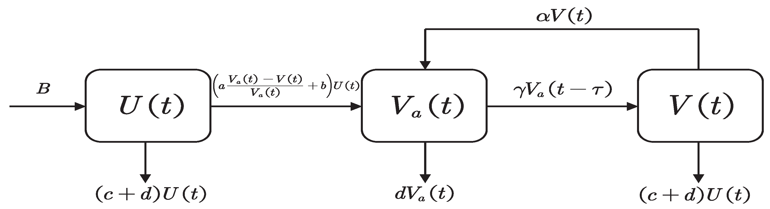
2. Mathematical Modeling

In Section 2, we will elaborate the model. The modeling in this paper is based on the dynamic process of COVID-19 vaccination.

First, we divide and explain the research object. When studying the process, we divide the sample population into three categories: The first type of sample U is an unvaccinated group, that is, the first type of population U is unvaccinated and does not have antibodies, which is recorded as unvaccinated population U. We do not consider that a small number of people have antibodies against COVID-19, so the second type of sample $V_a$ is a vaccinated group, that is, the second type of population $V_a$ is vaccinated and has antibodies, which is recorded as the vaccinated population $V_a$. The third type of sample V is the vaccine ineffective group, that is, the third type of population V has been vaccinated, but the antibody has disappeared, which is recorded as the ineffective population V.

Then, we briefly analyze the role relationship between the groups. Since COVID-19 antibodies have no maternal genetic characteristics, newborn population B is transferred to unvaccinated population U. Unvaccinated population U can become vaccinated population $V_a$ by being vaccinated against COVID-19. The vaccinated population $V_a$ may become ineffective population V due to the disappearance of antibodies after a period of time, and the vaccinated population $V_a$ can be inoculated with booster injection to prolong the time of antibody disappearance. Ineffective population V can also become vaccinated population $V_a$ through secondary vaccination with the COVID-19 vaccine. We assume that there is a vaccinated population $V_a$ that may contract COVID-19 but not die. Thus, we obtain the relationship between three populations (unvaccinated population (U), vaccinated population ($V_a$), and ineffective population (V), as shown in Figure 1:

In Figure 1, $U,V_a,V$ represent the sample numbers of unvaccinated, vaccinated and antibody disappearance, respectively, and parameters B and d represent natural increase of population and death rate of the samples, respectively; c is mortality rate due to COVID-19; $\alpha$ represents the secondary vaccination rate from V to $V_a$; $\gamma$ is the failure rate from $V_a$ to V; a and b are the positive feedback coefficients and basic vaccination rate in the positive feedback mechanism from U to $V_a$. We need to emphasize that the parameters involved in Figure 1 are all normal numbers. Finally, it is important to note that there is $V_a>V$ in the vaccinated population.

Next, we analyze the meaning of time-delay $\tau$. For the process from inoculated population $V_a$ to ineffective population V, we analyze the existence of time delay from two aspects. On the one hand, the novel coronavirus we are working on is very close to influenza virus, and the half-life of influenza virus antibodies is only about six months [35]. On the other hand, studies have shown that the half-life of antibodies in patients with mild new coronations is only 36 days [36]. Therefore, it can be concluded that COVID-19 vaccine is a non-permanent immune vaccine and has the time $\tau$ of the wide range of antibody failure, that is to say, most recipients ($\gamma$) will have the situation of antibody disappearance after the time $\tau$.

Furthermore, we construct a positive feedback mechanism on vaccine effectiveness to characterize a dynamic COVID-19 vaccination rate. For a vaccination rate from unvaccinated population U to vaccinated population $V_a$, we believe that a COVID-19 vaccination rate is affected by the willingness of the population to vaccinate. Li et al. [37] conducted a sample survey of patients in a tertiary hospital in a city, and concluded that worry about the safety and effectiveness of the vaccine was the main reason of the unwillingness for the vaccination. In Sarwar et al.’s [38] study, a multi-criteria decision-making method known as an analytical hierarchical method was applied to determine the COVID-19 vaccination willingness level of the public. The analysis revealed that the determinants of willingness to uptake the COVID-19 vaccine were individual decision, vaccine origin, adapting to change, and perceived barriers’ high obstacles to vaccinating. In Liu et al.’s [39] article, it was shown that free vaccination significantly increased COVID-19 vaccination rates. Referring to the literature above, we use the ratio of the current ineffective population V and the vaccinated population $V_a$ to characterize the effectiveness and safety of COVID-19: a smaller ratio indicates that the vaccine is more effective and safe, whereas a larger ratio indicates that the vaccine is less effective. Moreover, we denote the influence factor of the effectiveness and safety of COVID-19 vaccines as a, and the combined influence of factors includes vaccine source, vaccine cost, and vaccination barriers as b, and we can regard it as the basic fixed vaccination rate b for a period of time. To sum up, we construct a positive feedback mechanism for U to $V_a$ in the vaccination rate: $\frac{a\left(V_a-V\right)}{V_a}+b$.

Finally, combined with Figure 1, we give the following dynamic model of COVID-19 vaccination:

$$\left\{\begin{array}{c}\dot{U}\left(t\right)=B-(c+d)U\left(t\right)-\frac{a{V}_a\left(t\right)-aV\left(t\right)}{V_a\left(t\right)}U\left(t\right)-bU\left(t\right),\hfill \\ {\dot{V}}_a\left(t\right)=\frac{a{V}_a\left(t\right)-aV\left(t\right)}{V_a\left(t\right)}U\left(t\right)+bU\left(t\right)-d{V}_a\left(t\right)-\gamma V_a(t-\tau )+\alpha V\left(t\right),\hfill \\ \dot{V}\left(t\right)=\gamma V_a(t-\tau )-\alpha V\left(t\right)-(c+d)V\left(t\right).\hfill \end{array}\right.$$

(1)

where U, $V_a$, V are descriptive variables; B, a, b, c, d, $\alpha$, $\gamma$ are parameters; and $\tau$ is the time-delay. The specific definitions are given in

Table 1. Descriptions of variables and parameters in the model (1).

Symbol	Descriptions
U	Number of unvaccinated individuals without antibodies
$V_a$	Number of vaccinated individuals who develop antibodies
V	Number of vaccinated individuals whose antibodies failed
B	Natural increase of population
a	Factor affecting vaccine safety and efficacy
d	Natural mortality rate
b	Basic fixed vaccination rate
c	Mortality rate due to COVID-19
$\alpha$	Conversion rate from V to $V_a$, secondary vaccination rate for COVID-19 vaccine
$\gamma$	The conversion rate from $V_a$ to V, the COVID-19 vaccine failure rate
$\tau$	The time-delay between antibody production and antibody disappearance

.

3. Stability Analysis of Equilibrium and Existence of Hopf Bifurcation

In this section, we consider Equation (1) and determine the existence and stability of the positive equilibrium. We consider the following assumption:

(H1) $b\left(\alpha +c+d\right)+a\left(\alpha +c+d-\gamma \right)\ge 0$.

When (H1) holds, system (1) has one positive equilibrium $P(U^{*},V_a^{*},V^{*})$, where

$$\begin{array}{c}{U}^{*}=\frac{B}{c+d}-\frac{B\left[b\left(\alpha +c+d\right)+a\left(\alpha +c+d-\gamma \right)\right]}{\left(c+d\right)\left[\left(\alpha +c+d\right)\left(b+c+d\right)+a\left(\alpha +c+d-\gamma \right)\right]},\hfill \\ V_a^{*}=\frac{\left(\alpha +c+d\right)V^{*}}{\gamma },\hfill \\ V^{*}=\frac{B\gamma \left[b\left(\alpha +c+d\right)+a\left(\alpha +c+d-\gamma \right)\right]}{\left[\left(\alpha +c+d\right)\left(b+c+d\right)+a\left(\alpha +c+d-\gamma \right)\right]\left[\left(c+d\right)\left(d+\gamma \right)+\alpha d\right]}.\hfill \end{array}$$

(2)

We calculate the characteristic equation for equilibrium $P(U^{*},V_a^{*},V^{*})$ as follows:

$${\mathrm{e}}^{-\lambda \tau }\left[A_1{\lambda }^2+B_1\lambda +C_1\right]+{\lambda }^3+D_1{\lambda }^2+E_1\lambda +F_1=0,$$

(3)

where

$$\begin{array}{cc}\hfill A_1=& \gamma ,\hfill \\ \hfill B_1=& \left(\frac{a{U}^{*}\gamma }{V_a^{*}}+2c\gamma +2d\gamma +b\gamma +\frac{a\gamma \left(V_a^{*}-V^{*}\right)}{V_a^{*}}\right),\hfill \\ \hfill C_1=& \left(c+d+b+\frac{a\left(V_a^{*}-V^{*}\right)}{V_a^{*}}\right)\left(\frac{a{U}^{*}\gamma }{V_a^{*}}+\gamma c+\gamma d\right)-\frac{a{U}^{*}\gamma }{V_a^{*}}\left(\frac{a\left(V_a^{*}-V^{*}\right)}{V_a^{*}}+b\right),\hfill \\ \hfill D_1=& \left(2c+3d+b+\alpha +\frac{a\left(V_a^{*}-V^{*}\right)}{V_a^{*}}-\frac{a{U}^{*}{V}^{*}}{{\left(V_a^{*}\right)}^2}\right),\hfill \\ \hfill E_1=& \left(c+d+b+\frac{a\left(V_a^{*}-V^{*}\right)}{V_a^{*}}\right)\left(2d-\frac{a{U}^{*}{V}^{*}}{{\left(V_a^{*}\right)}^2}+\alpha +c\right)+\left(d-\frac{a{U}^{*}{V}^{*}}{{\left(V_a^{*}\right)}^2}\right)\left(\alpha +c+d\right)\hfill \\ \hfill & -\left(\frac{a\left(V_a^{*}-V^{*}\right)}{V_a^{*}}+b\right)\left(\frac{a{U}^{*}{V}^{*}}{{\left(V_a^{*}\right)}^2}\right),\hfill \\ \hfill F_1=& \left(d-\frac{a{U}^{*}{V}^{*}}{{\left(V_a^{*}\right)}^2}\right)\left(\alpha +c+d\right)\left(c+d+b+\frac{a\left(V_a^{*}-V^{*}\right)}{V_a^{*}}\right)\hfill \\ \hfill & -\left(\frac{a\left(V_a^{*}-V^{*}\right)}{V_a^{*}}+b\right)\left[\frac{a{U}^{*}{V}^{*}}{{\left(V_a^{*}\right)}^2}\left(\alpha +c+d\right)\right],\hfill \end{array}$$

with $U^{*},V_a^{*},V^{*}$ are given in Equation (2).

When $\tau =0$, Equation (3) becomes

$${\lambda }^3+a_1{\lambda }^2+a_2\lambda +a_3=0,$$

(4)

where

$$\begin{array}{cc}\hfill a_1=& -\frac{a{U}^{*}{V}^{*}}{{\left(V_a^{*}\right)}^2}+\gamma +3d+2c+b+\frac{a\left(V_a^{*}-V^{*}\right)}{V_a^{*}}+\alpha ,\hfill \\ \hfill a_2=& \gamma \left(\frac{a{U}^{*}}{V_a^{*}}-\alpha \right)+\left(-\frac{a{U}^{*}{V}^{*}}{{\left(V_a^{*}\right)}^2}+2d+\alpha +c+\gamma \right)\left(c+d+b+\frac{a\left(V_a^{*}-V^{*}\right)}{V_a^{*}}\right)\hfill \\ \hfill & -\frac{a{U}^{*}{V}^{*}}{{\left(V_a^{*}\right)}^2}\left(\frac{a\left(V_a^{*}-V^{*}\right)}{V_a^{*}}+b\right)+\left(\alpha +c+d\right)\left(d+\gamma -\frac{a{V}^{*}{U}^{*}}{{\left(V_a^{*}\right)}^2}\right),\hfill \\ \hfill a_3=& \left(c+d+b+\frac{a\left(V_a^{*}-V^{*}\right)}{V_a^{*}}\right)\left[\left(\alpha +c+d\right)\left(d+\gamma -\frac{a{U}^{*}{V}^{*}}{{\left(V_a^{*}\right)}^2}\right)+\gamma \left(\frac{a{U}^{*}}{V_a^{*}}-\alpha \right)\right]\hfill \\ \hfill & -\left(\frac{a\left(V_a^{*}-V^{*}\right)}{V_a^{*}}+b\right)\left[\frac{a\gamma U^{*}}{V_a^{*}}+\frac{a{U}^{*}{V}^{*}}{{\left(V_a^{*}\right)}^2}\left(\alpha +c+d\right)\right].\hfill \end{array}$$

According to the Routh–Hurwitz criterion, we consider the following assumption:

(H2) $a_1>0,a_3>0,a_1{a}_2-a_3>0$.

When (H2) holds, all the roots of Equation (4) have negative real parts, and the equilibrium $P(U^{*},V_a^{*},V^{*})$ is locally asymptotically stable when $\tau =0$.

When $\tau >0$, let $\lambda =\mathrm{i}\omega (\omega >0)$ be a root of Equation (3). Substituting $\lambda =\mathrm{i}\omega (\omega >0)$ into Equation (3) and separating the real and imaginary parts, we have:

$$\left\{\begin{array}{c}{\omega }^2{D}_1-F_1=-{\omega }^2{A}_{1}cos\left(\omega \tau \right)+C_{1}cos\left(\omega \tau \right)+\omega B_{1}sin\left(\omega \tau \right),\\ {\omega }^3-E_1\omega =\omega B_{1}cos\left(\omega \tau \right)+{\omega }^2{A}_{1}sin\left(\omega \tau \right)-C_{1}sin\left(\omega \tau \right).\end{array}\right.$$

(5)

Equation (5) leads to

$$\left\{\begin{array}{c}cos\left(\omega \tau \right)=\frac{m_2{\omega }^3+D_1{m}_1{\omega }^2-E_1{m}_2\omega -F_1{m}_1}{\gamma \left(m_1^2+m_2^2\right)},\hfill \\ sin\left(\omega \tau \right)=\frac{-m_1{\omega }^3+D_1{m}_2{w}^2+E_1{m}_1\omega -F_1{m}_2}{\gamma \left(m_1^2+m_2^2\right)},\hfill \end{array}\right.$$

(6)

where $m_1=\frac{-A_1{\omega }^2+C_1}{\gamma }$ and $m_2=\frac{B_1\omega }{\gamma }$.

Adding the square of two equations of Equation (5), and let ${\omega }^2=z$, we can obtain

$$h\left(z\right)=z^3+c_2{z}^2+c_{1}z+c_0,$$

(7)

where $c_2=\left(D_1^2-2E_1-A_1^2\right)$, $c_1=-\left(2F_1{D}_1-2A_1{C}_1+B_1^2-E_1^2\right)$, $c_0=F_1^2-C_1^2$.

We calculate the derivative of $h\left(z\right)$ to obtain $h^{\prime }\left(z\right)=3z^2+2c_{2}z+c_1$. When $\Delta =4{\left(c_2\right)}^2-12c_1>0$, and letting ${\tilde{z}}_1, {\tilde{z}}_2$ be the root of $h^{\prime }\left(z\right)=3z^2+2c_{2}z+c_1=0$, suppose ${\tilde{z}}_1<{\tilde{z}}_2$, thus ${\tilde{z}}_1=\frac{-2c_2+\sqrt{c_2^2-3c_1}}{3}$ and ${\tilde{z}}_2=\frac{-2c_2-\sqrt{c_2^2-3c_1}}{3}$.

Therefore, we give the following assumptions:

(H3) $c_0<0$, and satisfies $\Delta \le 0$ or $c_1\le 0$ or $c_2\ge 0$ or $h\left({\tilde{z}}_1\right)·h\left({\tilde{z}}_2\right)\ge 0$.

If (H3) holds, then Equation (7) has only one positive root $z_1$.

(H4) $c_0>0, \Delta >0, c_1>0, c_2<0, h\left({\tilde{z}}_2\right)<0$ or $c_0>0, \Delta >0, c_1<0, h\left({\tilde{z}}_2\right)<0.$

If (H4) holds, then Equation (7) has two positive roots $z_2$ and $z_3$.

(H5)  $c_0<0, \Delta >0, c_1>0, c_2<0, h\left({\tilde{z}}_1\right)·h\left({\tilde{z}}_2\right)<0.$

If (H5) holds, then Equation (7) has three positive roots $z_4$, $z_5$ and $z_6$.

In general, substituting ${\omega }_k=\sqrt{z_k}(k=1,2,···,6)$ into Equation (6), we obtain

$$\begin{array}{c}\hfill {\tau }_k^{\left(j\right)}=\left\{\begin{array}{cc}\frac{1}{{\omega }_k}[arccos\left(P_k\right)+2j\pi ],\hfill & Q_k\ge 0,\hfill \\ \frac{1}{{\omega }_k}[2\pi -arccos\left(P_k\right)+2j\pi ],\hfill & Q_k<0,k=1,2,···,6;j=0,1,2,\cdots ,\hfill \end{array}\right.\end{array}$$

(8)

where

$$\begin{array}{c}{Q}_k=sin({\omega }_k{\tau }_k^{\left(j\right)})=\frac{-m_1{\omega }_k^3+D_1{m}_2{w}_k^2+E_1{m}_1{\omega }_k-F_1{m}_2}{\gamma \left(m_1^2+m_2^2\right)},\\ P_k=cos({\omega }_k{\tau }_k^{\left(j\right)})=\frac{m_2{\omega }_k^3+D_1{m}_1{w}_k^2-E_1{m}_2{\omega }_k-F_1{m}_1}{\gamma \left(m_1^2+m_2^2\right)}.\end{array}$$

We discuss the number of positive roots of Equation (7) of the characteristic equation based on the above, and thus synthesize the following Lemma:

Lemma 1.

If  (H3)  or  (H4)  or  (H5)  holds, then Equation (3) has a pair of pure imaginary roots $\pm \mathrm{i}{\omega }_k$ when $\tau ={\tau }_k^{\left(j\right)}(k=1,2,···,6;j=0,1,2,\cdots )$, and all the other roots of Equation (3) have nonzero real parts.

Furthermore, let $\lambda \left(\tau \right)=\alpha \left(\tau \right)+\mathrm{i}\omega \left(\tau \right)$ be the root of Equation (3) satisfying $\alpha ({\tau }_k^{\left(j\right)})=0$, $\omega ({\tau }_k^{\left(j\right)})={\omega }_k(k=1,2,···,6;j=0,1,2,\cdots )$. Then, we consider the transversality condition.

Next, we derive both sides of the characteristic Equation (3) with respect to $\tau$ and solve for

$$\mathrm{Re}(\frac{\mathrm{d}\tau }{\mathrm{d}\lambda })=\frac{3z^2+2c_{2}z+c_1}{B_1^{2}z+{\left(C_1-A_{1}z\right)}^2}.$$

which gives us $\mathrm{Re}{\left(\frac{\mathrm{d}\lambda }{\mathrm{d}\tau }\right)}^{-1}=\mathrm{Re}\left(\frac{\mathrm{d}\tau }{\mathrm{d}\lambda }\right)$. Then, we have the following Lemma:

Lemma 2.

If  (H3)  or  (H4)  or  (H5)  holds, and $z_k={\omega }_k^2$, $h^{\prime }\left(z_k\right)\ne 0$, then we have the following transversality conclusions:

$${\left.\mathrm{Re}{(\frac{\mathrm{d}\lambda }{\mathrm{d}\tau })}^{-1}\right|}_{\tau ={\tau }_j^{\left(k\right)}}={\left.\mathrm{Re}(\frac{\mathrm{d}\tau }{\mathrm{d}\lambda })\right|}_{\tau ={\tau }_j^{\left(k\right)}}=\frac{h^{\prime }\left(z_k\right)}{B_1^2{z}_k+{\left(C_1-A_1{z}_k\right)}^2}\ne 0.$$

where $k=1,2,···,6;j=0,1,2,\cdots$ and $A_1,B_1$ and $C_1$ are given in Equation (3).

Based on the above conclusions, Lemmas 1 and 2, we obtain the following Theorem:

Theorem 1.

Based on the assumptions  (H1)  and  (H2)  hold, we show the conclusion associated with the equilibrium $P(U^{*},V_a^{*},V^{*})$ of the system (1). If one of three assumptions  (H3),  (H4), and  (H5)  holds, the equilibrium of system (1) undergoes the Hopf bifurcation at $\tau ={\tau }_k^{\left(j\right)}(k=1,2,···,6;j=0,1,2,\cdots )$, where ${\tau }_k^{\left(j\right)}$ is given by Equation (8), and

(1) If the assumptions  (H1)  and  (H2)  and  (H3)  hold, $h\left(z\right)$ has one positive root, then, when $\tau \in [0,{\tau }_1^{\left(0\right)})$, the equilibrium $P(U^{*},V_a^{*},V^{*})$ is locally asymptotically stable, and the equilibrium $P(U^{*},V_a^{*},V^{*})$ is unstable when $\tau >{\tau }_1^{\left(0\right)}$.

(2) If the assumptions  (H1)  and  (H2)  and  (H4)  hold, $h\left(z\right)$ has two positive roots, we suppose $z_2<z_3$, then $h^{\prime }\left(z_2\right)<0,h^{\prime }\left(z_3\right)>0$, note that ${\tau }_2^{\left(0\right)}>{\tau }_3^{\left(0\right)}$. Then, there exists $m\in N$ such that $0<{\tau }_3^{\left(0\right)}<{\tau }_2^{\left(0\right)}<{\tau }_3^{\left(1\right)}<{\tau }_2^{\left(1\right)}<\cdots <{\tau }_2^{(m-1)}<{\tau }_3^{\left(m\right)}<{\tau }_3^{(m+1)}$. When $\tau \in [0,{\tau }_3^{\left(0\right)})\cup {\displaystyle \bigcup _{l=1}^m}({\tau }_2^{(l-1)},{\tau }_3^{\left(l\right)})$, the equilibrium $P(U^{*},V_a^{*},V^{*})$ of the system (1) is locally asymptotically stable, and, when $\tau \in {\displaystyle \bigcup _{l=0}^{m-1}}({\tau }_3^{\left(l\right)},{\tau }_2^{\left(l\right)})\cup ({\tau }_3^{\left(m\right)},+\infty )$, the equilibrium $P(U^{*},V_a^{*},V^{*})$ is unstable.

(3) If the assumptions  (H1)  and  (H2)  and  (H5)  hold, $h\left(z\right)$ has three positive roots, and system (1) will generate stability switches similar to the above case (2).

4. Normal Form of Hopf Bifurcation

In this section, we calculate the normal form of Hopf bifurcation for the system (1) by using the multiple time scales method. In this paper, $\tau$ is the time delay between vaccination and vaccine failure, which has an important influence on model stability. Thus, we choose the time-delay $\tau$ as a bifurcation parameter, denoting $\tau ={\tau }_c+\epsilon {\tau }_{\epsilon }$, where ${\tau }_c$ is the critical value of Hopf bifurcation give in Equation (8), ${\tau }_{\epsilon }$ is the disturbance parameter, and $\epsilon$ is the dimensionless scale parameter. Note that, when $\tau ={\tau }_c$, the characteristic Equation (3) has eigenvalue $\lambda =\mathrm{i}\omega$, and system (1) undergoes a Hopf bifurcation near equilibrium $P(U^{*},V_a^{*},V^{*})$.

The system (1) can be written as $\dot{X}\left(t\right)=AX\left(t\right)+BX\left(t-\tau \right)+F\left(X\left(t\right),X\left(t-\tau \right)\right),$ and let $t\to t/\tau$, thus obtaining system (9):

$$\dot{X}=\tau AX+B\tau X\left(t-1\right)+\tau F\left(X,X\left(t-1\right)\right).$$

(9)

where $A:={\left(a_{ij}\right)}_{3\times 3}=\left(\begin{array}{ccc}\frac{a{V}^{*}}{V_a^{*}}-a-b-c-d& -\frac{a{V}^{*}{U}^{*}}{{\left(V_a^{*}\right)}^2}& \frac{a{U}^{*}}{V_a^{*}}\\ a+b-\frac{a{V}^{*}}{V_a^{*}}& \frac{a{U}^{*}{V}^{*}}{{\left(V_a^{*}\right)}^2}-d& \alpha -\frac{a{U}^{*}}{V_a^{*}}\\ 0& 0& -\left(\alpha +c+d\right)\end{array}\right),$ $B=\left(\begin{array}{ccc}0& 0& 0\\ 0& -\gamma & 0\\ 0& \gamma & 0\end{array}\right),$

$$\begin{array}{cc}\hfill & F\left(X\left(t\right),X\left(t-\tau \right)\right):=\left(\begin{array}{c}{F}_U\\ F_{V_a}\\ F_V\end{array}\right)\hfill \\ \hfill =& \left(\begin{array}{c}-\frac{V^{*}U{V}_a}{{\left(V_a^{*}\right)}^2}+\frac{aUV}{V_a^{*}}-\frac{a{U}^{*}{V}_{a}V}{{\left(V_a^{*}\right)}^2}+\frac{a{V}^{*}{U}^{*}{V}_a^2}{{\left(V_a^{*}\right)}^3}-\frac{a{V}^{*}{U}^{*}{V}_a^3}{{\left(V_a^{*}\right)}^4}+\frac{a{V}^{*}U{V}_a^2}{{\left(V_a^{*}\right)}^3}+\frac{a{U}^{*}V{V}_a^2}{{\left(V_a^{*}\right)}^3}-\frac{aU{V}_{a}V}{{\left(V_a^{*}\right)}^2}\\ \frac{V^{*}U{V}_a}{{\left(V_a^{*}\right)}^2}-\frac{aUV}{V_a^{*}}+\frac{a{U}^{*}{V}_{a}V}{{\left(V_a^{*}\right)}^2}-\frac{a{V}^{*}{U}^{*}{V}_a^2}{{\left(V_a^{*}\right)}^3}+\frac{a{V}^{*}{U}^{*}{V}_a^3}{{\left(V_a^{*}\right)}^4}-\frac{a{V}^{*}U{V}_a^2}{{\left(V_a^{*}\right)}^3}-\frac{a{U}^{*}V{V}_a^2}{{\left(V_a^{*}\right)}^3}+\frac{aU{V}_{a}V}{{\left(V_a^{*}\right)}^2}\\ 0\end{array}\right).\hfill \end{array}$$

We suppose h and $h^{*}$ are the eigenvector of the corresponding eigenvalue $\lambda =\mathrm{i}\omega {\tau }_c, \lambda =-\mathrm{i}\omega {\tau }_c$, respectively, of system (1) for equilibrium P, and satisfies $〈h^{*},h〉=\overline{{\left(h^{*}\right)}^T}·h=1$. By simple calculation, we can obtain:

$$\begin{array}{c}h:=\left(\begin{array}{c}{h}_1\\ h_2\\ h_3\end{array}\right)=\left(\begin{array}{c}\frac{\left(\mathrm{i}\omega +\left(d-\frac{a{V}^{*}{U}^{*}}{{\left(V_a^{*}\right)}^2}\right){\tau }_c+\gamma {\mathrm{e}}^{-\mathrm{i}\omega }{\tau }_c\right)\left(i\omega +\left(\alpha +c+d\right){\tau }_c\right)+\left(\frac{a{U}^{*}}{V_a^{*}}-\alpha \right)\gamma {\tau }_c^2{\mathrm{e}}^{-\mathrm{i}\omega }}{\gamma {\mathrm{e}}^{-\mathrm{i}\omega }\left(a+b-\frac{a{V}^{*}}{V_a^{*}}\right){\tau }_c^2}\\ \frac{i\omega +\left(\alpha +c+d\right){\tau }_c}{\gamma {\mathrm{e}}^{-\mathrm{i}\omega }{\tau }_c}\\ 1\end{array}\right),\hfill \\ h^{*}:=\left(\begin{array}{c}{h}_1^{*}\\ h_2^{*}\\ h_3^{*}\end{array}\right)=d_1\left(\begin{array}{c}1\\ \frac{\mathrm{i}\omega -\left(a+b+c+d-\frac{a{V}^{*}}{V_a^{*}}\right){\tau }_c}{\left(\frac{a{V}^{*}}{V_a^{*}}-a-b\right){\tau }_c}\\ \frac{\left(\frac{a{U}^{*}}{V_a^{*}}-\alpha \right)\left(\mathrm{i}\omega -\left(a+b+c+d-\frac{a{V}^{*}}{V_a^{*}}\right){\tau }_c\right)-\frac{a{U}^{*}{\tau }_c^2}{V_a^{*}}\left(\frac{a{V}^{*}}{V_a^{*}}-a-b\right)}{\left(\mathrm{i}\omega -\left(\alpha +c+d\right){\tau }_c\right)\left(\frac{a{V}^{*}}{V_a^{*}}-a-b\right){\tau }_c}\end{array}\right),\hfill \end{array}$$

(10)

where

$$\begin{array}{c}\lambda =\mathrm{i}\omega {\tau }_c,\hfill \\ d_1=\frac{\left(\lambda -\left(\alpha +c+d\right){\tau }_c\right)\left(\frac{a{V}^{*}}{V_a^{*}}-a-b\right)\gamma {\mathrm{e}}^{\lambda }{\tau }_c}{v_1+v_2+v_3+v_4},\hfill \\ v_1=\left(-2\lambda +\left(a+b+c+2d-\frac{a{V}^{*}{U}^{*}}{{\left(V_a^{*}\right)}^2}-\frac{a{V}^{*}}{V_a^{*}}\right){\tau }_c+\gamma {\mathrm{e}}^{\lambda }\right){\left(\lambda -\left(\alpha +c+d\right){\tau }_c\right)}^2,\hfill \\ v_2=\gamma {\tau }_c{\mathrm{e}}^{\lambda }\left(\alpha -\frac{a{U}^{*}}{V_a^{*}}\right)\left(\lambda -\left(\alpha +c+d\right){\tau }_c\right),\hfill \\ v_3=\gamma {\mathrm{e}}^{\lambda }\left(\frac{a{U}^{*}}{V_a^{*}}-\alpha \right)\left(\lambda -\left(a+b+c+d-\frac{a{V}^{*}}{V_a^{*}}\right){\tau }_c\right),\hfill \\ v_4=-\frac{a{U}^{*}{\tau }_c^2\gamma {\mathrm{e}}^{\lambda }}{V_a^{*}}\left(\frac{a{V}^{*}}{V_a^{*}}-a-b\right).\hfill \end{array}$$

We suppose the solution of system (4.1) as follows:

$$X\left(t\right)=X\left(T_0,T_1,T_2,···\right)=\sum _{k=1}^{\infty }{\epsilon }^k{X}_k\left(T_0,T_1,T_2,···\right).$$

(11)

The derivative with respect to t is transformed into:

$$\frac{d}{dt}=\frac{\partial }{\partial T_0}+\epsilon \frac{\partial }{\partial T_1}+{\epsilon }^2\frac{\partial }{\partial T_2}+···=D_0+\epsilon D_1+{\epsilon }^2{D}_2+···,$$

where $D_i=\frac{\partial }{\partial T_i}$, i=0,1,2$···$.

Note that

$$\begin{array}{c}{X}_i={(U_i,V_{a_i},V_i)}^T=X_i\left(t,\epsilon t,{\epsilon }^{2}t,···\right),\hfill \\ X_{i1}={\left(U_{i1},V_{a_{i1}},V_{i1}\right)}^T=X_i\left(t-1,\epsilon t,{\epsilon }^{2}t,···\right),i=1,2,···.\hfill \end{array}$$

Then, we can obtain:

$$\dot{X}\left(t\right)=\epsilon D_0{X}_1+{\epsilon }^2{D}_1{X}_1+{\epsilon }^3{D}_2{X}_1+{\epsilon }^2{D}_0{X}_2+{\epsilon }^3{D}_1{X}_2+{\epsilon }^3{D}_0{X}_3+···.$$

(12)

By Taylor expansion of $X\left(t-1\right)$ at $X_i\left(t-1,\epsilon t,{\epsilon }^{2}t,···\right)$, we obtain that

$$X\left(t-1\right)=\epsilon X_{11}+{\epsilon }^2\left(X_{21}-D_1{X}_{11}\right)+{\epsilon }^3\left(X_{31}-D_1{X}_{21}-D_2{X}_{11}\right)+···,$$

(13)

where $X_{i1}=X_i\left(T_0-1,T_1,T_2,···\right),i=1,2,3,···.$

We consider that $\tau$ is the bifurcation parameter, and we set $\tau ={\tau }_c+\epsilon {\tau }_{\epsilon }$, where ${\tau }_k^{\left(j\right)}$ is the critical value of the Hopf bifurcation, ${\tau }_{\epsilon }$ is the perturbation parameter, and $\epsilon$ is the dimensionless parameter. Substituting Equations (11)–(13) into Equation (9), and comparing the coefficients before $\epsilon$, we obtain the following equation:

$$\begin{array}{c}{D}_0{U}_1-{\tau }_c\left(a_{11}{U}_1+a_{12}{V}_{a_1}+a_{13}{V}_1\right)=0,\hfill \\ D_0{V}_{a_1}-{\tau }_c\left(a_{21}{U}_1+a_{22}{V}_{a_1}+a_{23}{V}_1\right)+{\tau }_c{V}_{a_{11}}\gamma =0,\hfill \\ D_0{V}_1-{\tau }_c{a}_{33}{V}_1-{\tau }_c{V}_{a_{11}}\gamma =0.\hfill \end{array}$$

(14)

Then, we have the solution of Equation (14):

$$X_1\left(T_1,T_2,T_3,···\right)=G\left(T_1,T_2,T_3,···\right){\mathrm{e}}^{i\omega {\tau }_c{T}_0}h+\overline{G}\left(T_1,T_2,T_3,···\right){\mathrm{e}}^{-i\omega {\tau }_c{T}_0}\overline{h}.$$

(15)

where h is given in Equation (10).

The expression of the coefficient before ${\epsilon }^2$ is as follows:

$$\begin{array}{c}\begin{array}{cc}\hfill & D_0{U}_2-{\tau }_c\left(a_{11}{U}_2+a_{12}{V}_{a_2}+a_{13}{V}_2\right)\hfill \\ \hfill =& -D_1{U}_1+{\tau }_{\epsilon }\left(a_{11}{U}_1+a_{12}{V}_{a_1}+a_{13}{V}_1\right)-\frac{V^{*}}{{\left(V_a^{*}\right)}^2}{U}_1{V}_{a_1}{\tau }_c\hfill \\ \hfill & +\frac{a}{V_a^{*}}{U}_1{V}_1{\tau }_c-\frac{a{U}^{*}}{{\left(V_a^{*}\right)}^2}{V}_{a_1}{V}_1{\tau }_c+\frac{a{V}^{*}{U}^{*}}{{\left(V_a^{*}\right)}^3}{V}_{a_1}^2{\tau }_c,\hfill \\ \hfill & D_0{V}_{a_2}-{\tau }_c\left(a_{21}{U}_2+a_{22}{V}_{a_2}+a_{23}{V}_2\right)+{\tau }_c{V}_{a_{21}}\gamma \hfill \\ \hfill =& -D_1{V}_{a_1}+{\tau }_c\left(\frac{V^{*}{U}_1{V}_{a_1}}{{\left(V_a^{*}\right)}^2}-\frac{a{U}_1{V}_1}{V_a^{*}}+\frac{a{U}^{*}{V}_{a_1}{V}_1}{{\left(V_a^{*}\right)}^2}-\frac{a{V}^{*}{U}^{*}{V}_{a_1}^2}{{\left(V_a^{*}\right)}^3}+\gamma D_1{V}_{a_{11}}\right)\hfill \\ \hfill & +{\tau }_{\epsilon }\left(a_{21}{U}_1+a_{22}{V}_{a_1}+a_{23}{V}_1-\gamma V_{a_{11}}\right),\hfill \\ \hfill & D_0{U}_2-{\tau }_c{a}_{33}{V}_2-{\tau }_c\gamma V_{a_{21}}=-D_1{V}_1+{\tau }_{\epsilon }{a}_{33}{V}_1-{\tau }_c\gamma D_1{V}_{a_{11}}+{\tau }_{\epsilon }\gamma V_{a_{11}}.\hfill \end{array}\hfill \end{array}$$

(16)

Substituting Equation (15) into the right-hand side of Equation (16), the coefficient vector of ${\mathrm{e}}^{i\omega T_0}$ is denoted by $m_3$. According to the solvability condition, the expression of $\frac{\partial G}{\partial T_1}$ can be obtained as follows:

$$\frac{\partial G}{\partial T_1}=K{\tau }_{\epsilon }G,$$

(17)

where $K=\frac{a_{11}{h}_1\overline{h_1^{*}}+a_{12}{h}_2\overline{h_1^{*}}+a_{13}{h}_3\overline{h_1^{*}}+a_{21}{h}_1\overline{h_2^{*}}+a_{22}{h}_2\overline{h_2^{*}}+a_{23}{h}_3\overline{h_2^{*}}-\gamma {\mathrm{e}}^{-i\omega {\tau }_c}{h}_2\overline{h_2^{*}}+a_{33}{h}_3\overline{h_3^{*}}+\gamma {\mathrm{e}}^{-i\omega {\tau }_c}{h}_2\overline{h_3^{*}}}{1+\gamma {\tau }_c\left(h_2\overline{h_3^{*}}-h_2\overline{h_2^{*}}\right){\mathrm{e}}^{-i\omega {\tau }_c}}$.

${\tau }_{\epsilon }$ is a small disturbance parameter, and it has little effect on the high order. Thus, we only consider its effect on the linear part. We suppose the solution of Equation (16) is as follows:

$$\begin{array}{cc}\hfill & U_2=g_1{\mathrm{e}}^{2i\omega {\tau }_c{T}_0}{G}^2+\overline{g_1}{\mathrm{e}}^{-2i\omega {\tau }_c{T}_0}{\overline{G}}^2+l_{1}G\overline{G},\hfill \\ \hfill & V_{a_2}=g_2{\mathrm{e}}^{2i\omega {\tau }_c{T}_0}{\overline{G}}^2+\overline{g_2}{\mathrm{e}}^{-2i\omega {\tau }_c{T}_0}{\overline{G}}^2+l_{2}G\overline{G},\hfill \\ \hfill & V_2=g_3{\mathrm{e}}^{2i\omega {\tau }_c{T}_0}{G}^2+\overline{g_3}{\mathrm{e}}^{-2i\omega {\tau }_c{T}_0}{\overline{G}}^2+l_{3}G\overline{G}.\hfill \end{array}$$

(18)

Substituting Equation (18) into Equation (16), we obtain:

$$\left(\begin{array}{c}{g}_1\\ g_2\\ g_3\end{array}\right)=\frac{A_2^{*}}{\left|A_2\right|}\left(\begin{array}{c}{y}_1^1\\ y_2^1\\ y_3^1\end{array}\right),\left(\begin{array}{c}{l}_1\\ l_2\\ l_3\end{array}\right)=\frac{A_3^{*}}{\left|A_3\right|}\left(\begin{array}{c}{y}_1^2\\ y_2^2\\ y_3^2\end{array}\right),$$

(19)

where

$$\begin{array}{c}{y}_1^1=-\frac{V^{*}}{{\left(V_a^{*}\right)}^2}{h}_1{h}_2+\frac{a}{V_a^{*}}{h}_1{h}_3-\frac{a{U}^{*}}{{\left(V_a^{*}\right)}^2}{h}_2{h}_3+\frac{a{V}^{*}{U}^{*}}{{\left(V_a^{*}\right)}^3}{h}_1^2,\hfill \\ y_2^1=\frac{V^{*}}{{\left(V_a^{*}\right)}^2}{h}_1{h}_2-\frac{a}{V_a^{*}}{h}_1{h}_3+\frac{a{U}^{*}}{{\left(V_a^{*}\right)}^2}{h}_2{h}_3-\frac{a{V}^{*}{U}^{*}}{{\left(V_a^{*}\right)}^3}{h}_1^2,\hfill \\ y_3^1=0.\hfill \\ y_1^2=\frac{V^{*}}{{\left(V_a^{*}\right)}^2}\left(h_1\overline{h_2}+\overline{h_1}{h}_2\right)-\frac{a}{V_a^{*}}\left(h_1\overline{h_3}+\overline{h_1}{h}_3\right)+\frac{a{U}^{*}}{{\left(V_a^{*}\right)}^2}\left(h_2\overline{h_3}+\overline{h_2}{h}_3\right)-\frac{2a{V}^{*}{U}^{*}}{{\left(V_a^{*}\right)}^3}{h}_1\overline{h_1},\hfill \\ y_2^2=-\frac{V^{*}}{{\left(V_a^{*}\right)}^2}\left(h_1\overline{h_2}+\overline{h_1}{h}_2\right)+\frac{a}{V_a^{*}}\left(h_1\overline{h_3}+\overline{h_1}{h}_3\right)-\frac{a{U}^{*}}{{\left(V_a^{*}\right)}^2}\left(h_2\overline{h_3}+\overline{h_2}{h}_3\right)+\frac{2a{V}^{*}{U}^{*}}{{\left(V_a^{*}\right)}^3}{h}_1\overline{h_1},\hfill \\ y_3^2=0.\hfill \\ A_k=\left(\begin{array}{ccc}{x}_{11}^k& x_{12}^k& x_{13}^k\\ x_{21}^k& x_{22}^k& x_{23}^k\\ x_{31}^k& x_{32}^k& x_{33}^k\end{array}\right)\hfill \\ A_k^{*}=\left(\begin{array}{ccc}{x}_{22}^k{x}_{33}^k-x_{32}^k{x}_{23}^k& -x_{21}^k{x}_{33}^k+x_{31}^k{x}_{23}^k& x_{21}^k{x}_{32}^k-x_{31}^k{x}_{22}^k\\ -x_{12}^k{x}_{33}^k+x_{32}^k{x}_{13}^k& x_{11}^k{x}_{33}^k-x_{31}^k{x}_{13}^k& -x_{11}^k{x}_{32}^k+x_{31}^k{x}_{12}^k\\ x_{12}^k{x}_{23}^k-x_{22}^k{x}_{13}^k& -x_{11}^k{x}_{23}^k+x_{21}^k{x}_{13}^k& x_{11}^k{x}_{22}^k-x_{21}^k{x}_{12}^k\end{array}\right)\hfill \\ \left|A_k\right|=x_{11}^k\left(x_{22}^k{x}_{33}^k-x_{32}^k{x}_{23}^k\right)-x_{12}^k\left(x_{21}^k{x}_{33}^k-x_{31}^k{x}_{23}^k\right)+x_{13}^k\left(x_{21}^k{x}_{32}^k-x_{31}^k{x}_{22}^k\right),k=1,2,3.\hfill \end{array}$$

with

$$\begin{array}{c}{x}_{11}^1=a+b+c+d-\frac{a{V}^{*}}{V_a^{*}}+i\omega ,x_{12}^1=\frac{a{V}^{*}{U}^{*}}{{\left(V_a^{*}\right)}^2},x_{13}^1=-\frac{a{U}^{*}}{V_a^{*}},\hfill \\ x_{21}^1=\frac{a{V}^{*}}{V_a^{*}}-a-b,x_{22}^1=d-\frac{a{V}^{*}{U}^{*}}{{\left(V_a^{*}\right)}^2}+i\omega +\gamma {\mathrm{e}}^{-i\omega {\tau }_c},x_{23}^1=\frac{a{U}^{*}}{V_a^{*}}-\alpha ,\hfill \\ x_{31}^1=0,x_{32}^1=-\gamma {\mathrm{e}}^{-i\omega {\tau }_c},x_{33}^1=\alpha +c+d+i\omega ,\hfill \\ x_{11}^2=a+b+c+d-\frac{a{V}^{*}}{V_a^{*}}+2i\omega ,x_{12}^2=\frac{a{V}^{*}{U}^{*}}{{\left(V_a^{*}\right)}^2},x_{13}^2=-\frac{a{U}^{*}}{V_a^{*}},\hfill \\ x_{21}^2=\frac{a{V}^{*}}{V_a^{*}}-a-b,x_{22}^2=d-\frac{a{V}^{*}{U}^{*}}{{\left(V_a^{*}\right)}^2}+2i\omega +\gamma {\mathrm{e}}^{-2i\omega {\tau }_c},x_{23}^2=\frac{a{U}^{*}}{V_a^{*}}-\alpha ,\hfill \\ x_{31}^2=0,x_{32}^2=-\gamma {\mathrm{e}}^{-2i\omega {\tau }_c},x_{33}^2=\alpha +c+d+2i\omega ,\hfill \\ x_{11}^3=\frac{a{V}^{*}}{V_a^{*}}-a-b-c-d,x_{12}^3=-\frac{a{V}^{*}{U}^{*}}{{\left(V_a^{*}\right)}^2},x_{13}^3=\frac{a{U}^{*}}{V_a^{*}},\hfill \\ x_{21}^3=a+b-\frac{a{V}^{*}}{V_a^{*}},x_{22}^3=\frac{a{V}^{*}{U}^{*}}{{\left(V_a^{*}\right)}^2}-d-\gamma ,x_{23}^3=\alpha -\frac{a{U}^{*}}{V_a^{*}},\hfill \\ x_{31}^3=0,x_{32}^3=\gamma ,x_{33}^3=-\alpha -c-d.\hfill \end{array}$$

The expression of the coefficient before ${\epsilon }^3$ is:

$$\begin{array}{cc}\hfill & \begin{array}{cc}& D_0{U}_3-{\tau }_c\left(a_{11}{U}_3+a_{12}{V}_{a_3}+a_{13}{V}_3\right)\hfill \\ \hfill =& -D_1{U}_2{D}_2{U}_1+{\tau }_{\epsilon }\left(a_{11}{U}_2+a_{12}{V}_{a_2}+a_{13}{V}_2\right)-\frac{V^{*}}{{\left(V_a^{*}\right)}^2}\left(U_1{V}_{a_1}{\tau }_{\epsilon }+U_1{V}_{a_2}{\tau }_c+U_2{V}_{a_1}{\tau }_c\right)\hfill \\ \hfill & +\frac{a}{V_a^{*}}\left(U_1{V}_1{\tau }_{\epsilon }+U_1{V}_2{\tau }_c+U_2{V}_1{\tau }_c\right)-\frac{a{U}^{*}}{{\left(V_a^{*}\right)}^2}\left(V_{a_1}{V}_1{\tau }_{\epsilon }+V_{a_1}{V}_2{\tau }_c+V_{a_2}{V}_1{\tau }_c\right)-\frac{a{V}^{*}{U}^{*}}{{\left(V_a^{*}\right)}^4}{V}_{a_1}^3{\tau }_c\hfill \\ \hfill & +\frac{a{V}^{*}{U}^{*}}{{\left(V_a^{*}\right)}^3}\left(V_{a_1}^2{\tau }_{\epsilon }+2V_{a_1}{V}_{a_2}{\tau }_c\right)+\frac{a{V}^{*}}{{\left(V_a^{*}\right)}^3}{U}_1{V}_{a_1}^2{\tau }_c+\frac{a{U}^{*}}{{\left(V_a^{*}\right)}^3}{V}_{a_1}^2{V}_1{\tau }_c-\frac{a}{{\left(V_a^{*}\right)}^2}{U}_1{V}_{a_1}{V}_1{\tau }_c,\hfill \end{array}\hfill \\ \hfill & \begin{array}{cc}& D_0{V}_{a_3}-{\tau }_c\left(a_{21}{U}_3+a_{22}{V}_{a_3}+a_{23}{V}_3\right)+{\tau }_c{V}_{a_{31}}\gamma \hfill \\ \hfill =& -D_1{V}_{a_2}-D_2{V}_{a_1}+{\tau }_{\epsilon }\left(a_{21}{U}_2+a_{22}{V}_{a_2}+a_{23}{V}_2\right)+\frac{V^{*}}{{\left(V_a^{*}\right)}^2}\left(U_1{V}_{a_1}{\tau }_{\epsilon }+U_1{V}_{a_2}{\tau }_c+U_2{V}_{a_1}{\tau }_c\right)\hfill \\ \hfill & -\frac{a}{V_a^{*}}\left(U_1{V}_1{\tau }_{\epsilon }+U_1{V}_2{\tau }_c+U_2{V}_1{\tau }_c\right)+\frac{a{U}^{*}}{{\left(V_a^{*}\right)}^2}\left(V_{a_1}{V}_1{\tau }_{\epsilon }+V_{a_1}{V}_2{\tau }_c+V_{a_2}{V}_1{\tau }_c\right)+\frac{a{V}^{*}{U}^{*}}{{\left(V_a^{*}\right)}^4}{V}_{a_1}^3{\tau }_c\hfill \\ \hfill & -\frac{a{V}^{*}{U}^{*}}{{\left(V_a^{*}\right)}^3}\left(V_{a_1}^2{\tau }_{\epsilon }+2V_{a_1}{V}_{a_2}{\tau }_c\right)-\frac{a{V}^{*}}{{\left(V_a^{*}\right)}^3}{U}_1{V}_{a_1}^2{\tau }_c-\frac{a{U}^{*}}{{\left(V_a^{*}\right)}^3}{V}_{a_1}^2{V}_1{\tau }_c+\frac{a}{{\left(V_a^{*}\right)}^2}{U}_1{V}_{a_1}{V}_1{\tau }_c\hfill \\ \hfill & +{\tau }_c\gamma D_1{V}_{a_{21}}+{\tau }_c\gamma D_2{V}_{a_{11}}-{\tau }_{\epsilon }\gamma \left(V_{a_{21}}-D_1{V}_{a_{11}}\right),\hfill \end{array}\hfill \\ \hfill & \begin{array}{cc}& D_0{V}_3-{\tau }_c{a}_{33}{V}_3-{\tau }_c\gamma V_{a_{31}}\hfill \\ \hfill =& -D_1{V}_2{D}_2{V}_1+{\tau }_{\epsilon }{a}_{33}{V}_2-{\tau }_c\gamma \left(D_1{V}_{a_{21}}+D_2{V}_{a_{11}}\right)+{\tau }_{\epsilon }\gamma \left(V_{a_{21}}-D_1{V}_{a_{11}}\right).\hfill \end{array}\hfill \end{array}$$

(20)

Substituting Equations (15), (18), and (19) into the right-hand side of Equation (20), and $m_4$ denotes the coefficient vector of ${\mathrm{e}}^{i\omega T_0}$. According to the solvability condition $〈h^{*},m_4〉=0$, and noting that ${\tau }_{\epsilon }^2$ is small enough for small unfolding parameter ${\tau }_{\epsilon }$, we ignore the term ${\tau }_{\epsilon }^{2}G$. Then, we have:

$$\frac{\partial G}{\partial T_2}=H{G}^2\overline{G},$$

(21)

where

$$\begin{array}{c}H=\frac{{\tau }_c\left(\overline{h_1^{*}}-\overline{h_2^{*}}\right){\sum }_{i=1}^4{H}_i}{1+{\tau }_c\gamma e^{-i\omega {\tau }_c}{h}_2\left(\overline{h_3^{*}}-\overline{h_2^{*}}\right)},\hfill \\ H_1=-\frac{V^{*}}{{\left(V_a^{*}\right)}^2}\left(h_1{l}_2+g_2\overline{h_1}+h_2{l}_1+\overline{h_2}G\right)+\frac{a}{V_a^{*}}\left(h_1{l}_3+\overline{h_1}{g}_3+h_3{l}_1+\overline{h_3}G\right),\hfill \\ H_2=-\frac{a{U}^{*}}{{\left(V_a^{*}\right)}^2}\left(h_2{l}_3+\overline{h_2}{g}_3+h_3{l}_2+\overline{h_3}{g}_2\right)+\frac{2a{V}^{*}{U}^{*}}{{\left(V_a^{*}\right)}^3}\left(h_2{l}_2+\overline{h_2}{g}_2\right),\hfill \\ H_3=-\frac{3a{V}^{*}{U}^{*}}{{\left(V_a^{*}\right)}^4}{h}_2^2\overline{h_2}+\frac{a{V}^{*}}{{\left(V_a^{*}\right)}^3}\left(2h_1{h}_2\overline{h_2}+\overline{h_1}{h}_2^2\right),\hfill \\ H_4=\frac{a{U}^{*}}{{\left(V_a^{*}\right)}^3}\left(2h_2\overline{h_2}{h}_3+h_2^2\overline{h_3}\right)-\frac{a}{{\left(V_a^{*}\right)}^2}\left(h_1{h}_2\overline{h_3}+h_1\overline{h_2}{h}_3+\overline{h_1}{h}_2{h}_3\right),\hfill \end{array}$$

where $g_k$ ( $k=1,2,3$ ) and $l_k$ ( $k=1,2,3$ ) are given in Equation (19), and $h_j$ ( $j=1,2,3$ ) and $h_j^{*}$ ( $j=1,2,3$ ) are given in Equation (10).

Letting $G\mapsto \left(G/\epsilon \right),$ we can obtain the normal form of Hopf bifurcation of system (1) as:

$$\dot{G}=K{\tau }_{\epsilon }G+H{G}^2\overline{G},$$

(22)

where K is given in Equation (17), and H is given in Equation (21).

Letting $G=r{\mathrm{e}}^{i\theta }$ and substituting it into Equation (22), and we can obtain the normal form of the Hopf bifurcation in polar coordinates:

$$\left\{\begin{array}{c}\dot{r}=\mathrm{Re}\left(K\right){\tau }_{\epsilon }r+\mathrm{Re}\left(H\right)r^3,\\ \dot{\theta }=\mathrm{Im}\left(K\right){\tau }_{\epsilon }+\mathrm{Im}\left(H\right)r^2,\end{array}\right.$$

(23)

where K is expressed in Equation (17), and H is expressed in Equation (21).

According to the normal form of the Hopf bifurcation by polar coordinates, we just need to consider the first equation by system (23). Thus, there is the following theorem:

Theorem 2.

For system (23), when $\frac{\mathrm{Re}\left(K\right){\tau }_{\epsilon }}{\mathrm{Re}\left(H\right)}<0$, there is a nontrivial fixed point $r=$$\sqrt{-\frac{\mathrm{Re}\left(K\right){\tau }_{\epsilon }}{\mathrm{Re}\left(H\right)}<0}$, and system (1) has periodic solution:

(1) If $\mathrm{Re}\left(K\right){\tau }_{\epsilon }<0$, then the periodic solution reduced on the center manifold is unstable.

(2) If $\mathrm{Re}\left(K\right){\tau }_{\epsilon }>0$, then the periodic solution reduced on the center manifold is stable.

5. Numerical Simulations

In this section, since different countries have different prevention and control strategies and basic national conditions, there are some differences in the parameters values taken in the corresponding models. We will complete the numerical simulations in two parts: the first part is the parameters analysis to estimate the required parameters range in the model and select two sets of parameters values within a reasonable parameters range; the second part is the numerical simulations and parameters discussion, using the two sets of reasonable parameters selected in the first part as an example and MATLAB for numerical simulations. In addition, based on the COVID-19 variant strains, the effect of each parameter on the critical time ${\tau }_1^{\left(0\right)}$ is discussed.

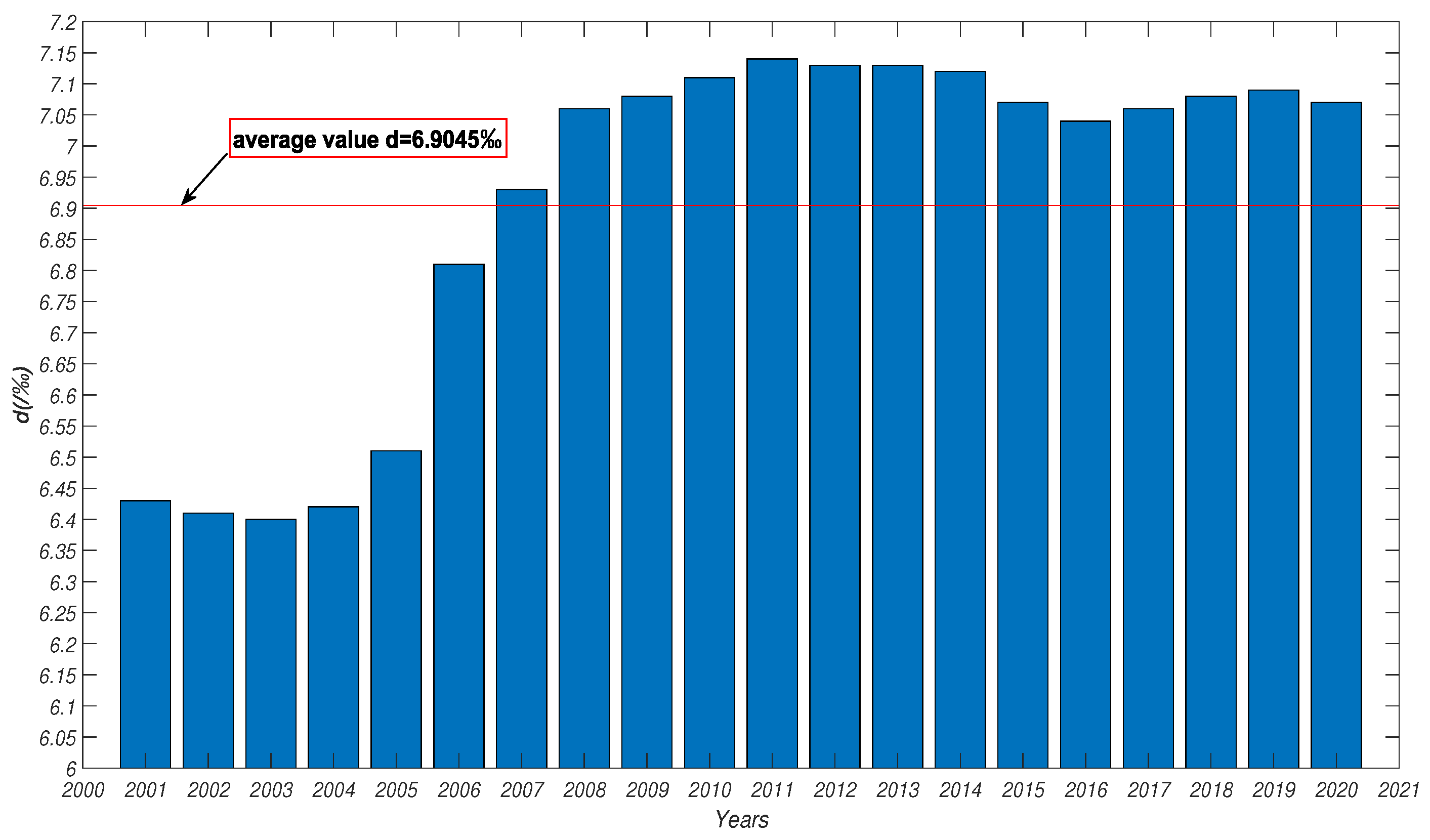
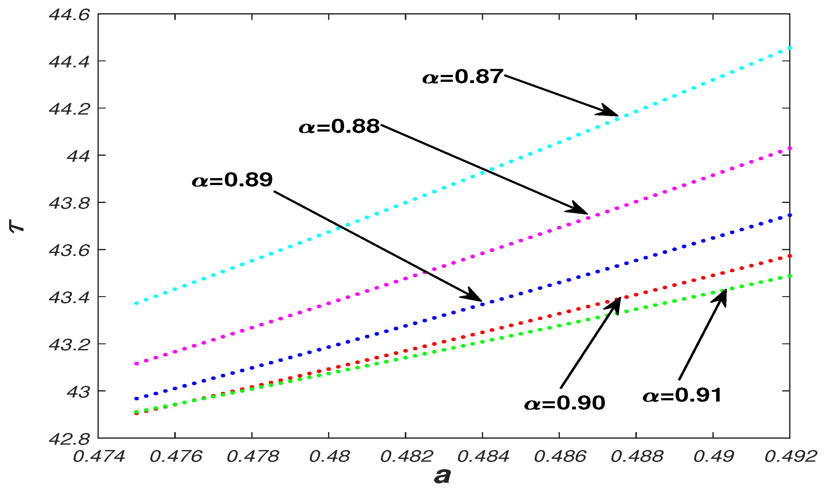
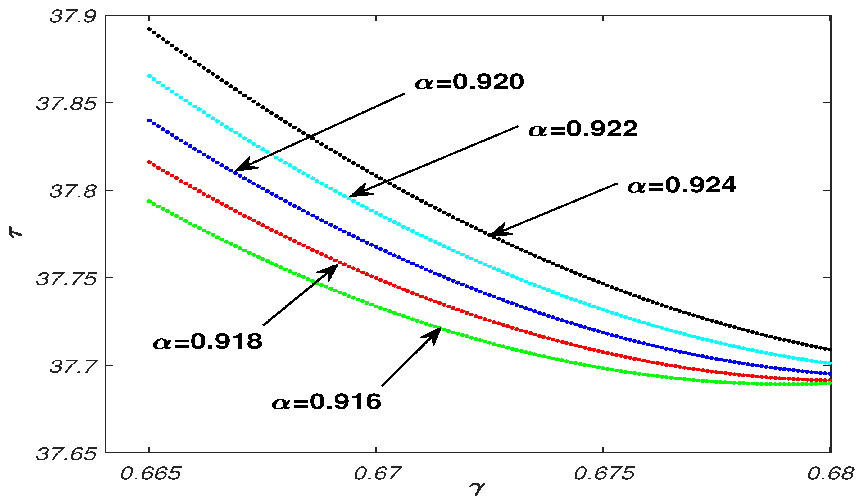
5.1. Parameter Analysis

In this part, we estimate some parameters used in numerical simulations to make them closer to the actual parameters. Then, we give estimates of natural birth rate $B_r$, disease-related death rate c, and natural death rate d. At the same time, we also made some reasonable assumptions about the large range of failure rate $\gamma$, the weight factor a, the fixed vaccination rate b, and the secondary vaccination rate $\alpha$.

First, for the natural birth rate, we select the natural birth rate of some countries in a certain year of Central Intelligence Agency (CIA) as the study data, and after excluding the outliers, we analyze the range of natural birth rate values roughly: $Br\in (0.770,1.250).$ Then, from the perspective of time change, we specifically analyze the change of natural birth rate $B_r$ in China in recent years by using the data from the National Bureau of Statistics of the People’s Republic of China (NBSPRC) as an example, and obtain that its mean value is within a reasonable interval. Analyze the world natural birth rate $B_r$ from two dimensions of region and time. Finally, we consider the population base as unit 1, and the natural increase of population B and the natural birth rate $B_r$ are numerically equal. Thus, the birth rate $B=1.120\%$ is selected as the simulations parameter.

Second, for COVID-19 disease-related mortality c, we select the data of Johns Hopkins University (https://coronavirus.jhu.edu/map.html, accessed on 12 December 2021) to observe the mortality due to illness, and then we find that different countries have large fluctuations. Therefore, we select some representative countries in a balanced way and analyze the value range of disease-related mortality c. Here, the data mean is used as the parameters in the next section, and the disease-related mortality $c=4.6550\%$ is obtained with general significance. It is important to note that the model applies equally to other reasonable values of the parameter c.

Next, as for the natural mortality rate d, the natural mortality rate of a country can be influenced by many aspects and varies greatly from country to country in practice. Therefore, when analyzing the natural mortality rate d, we select data from different countries in a balanced way for the analysis, and we take the data from the Intelligent Data Platform (https://mobile.hellobi.com, accessed on 14 December 2021) as an example, and excluding the abnormal mortality data in that year, we consider a reasonable interval for the natural mortality rate d: $d\in (4.5500,14.5000)$. For a better fit, the birth rate $B_r$ refers to the data from National Bureau of Statistics of the People’s Republic of China (NBSPRC), so the mortality rate is also selected partially from NBSPRC, as shown in Figure 2. Due to the large range of intervals, we select $d=0.6904\%$ and $d=1.4170\%$ for subsequent numerical simulations.

Finally, for parameters without numerical support, we select parameters values in the way of reasonable assumptions to carry out numerical simulations in the next section. In this model, for other assumed parameters, the model has stability and can give the model conclusion under reasonable parameters.

For large-range failure rate $\gamma$, the large-range is a catch-all term. Here, we believe that a failure rate greater than $0.5$ and less than 1 is identified as a large-scale failure rate. In the future numerical simulations, we will take the vicinity of $\gamma =0.67$ as an example for simulations.

As for the impact factor a and the fixed vaccination rate b, the values of a and b are greatly influenced by personal subjective consciousness and are also related to the publicity and encouragement policies of a country or region, but the relationship between a and b should be guaranteed: $a+b\le 1$. In the following simulations, we take both a and b near $0.5$ as an example.

For the secondary vaccination rate $\alpha$, we can make assumptions, the significance of which is to study the epidemic prevention and control effects under different secondary vaccination rate $\alpha$. In the simulations, we take $\alpha$ near $0.9$ as an example for numerical simulations.

In summary, the two groups of parameters used in the simulations results in the next section are as follows:

$I:B=0.0112, d=0.0069, c=0.04655, \gamma =0.675, a=0.49, b=0.5, \alpha =0.9$.

$II:B=0.0112, d=0.01417, c=0.04655, \gamma =0.685, a=0.49, b=0.5, \alpha =0.92$.

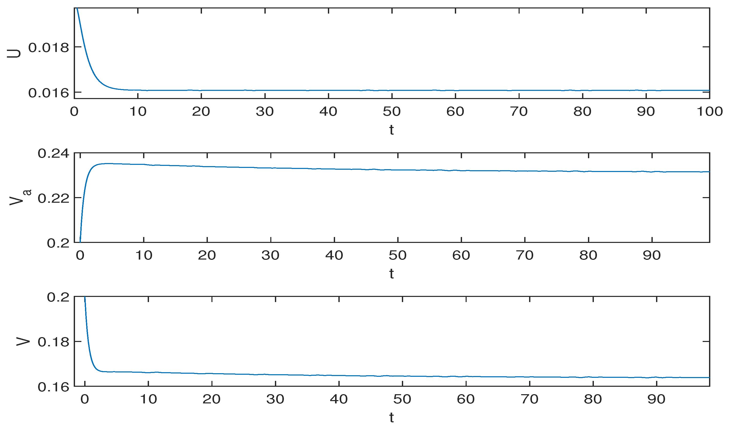
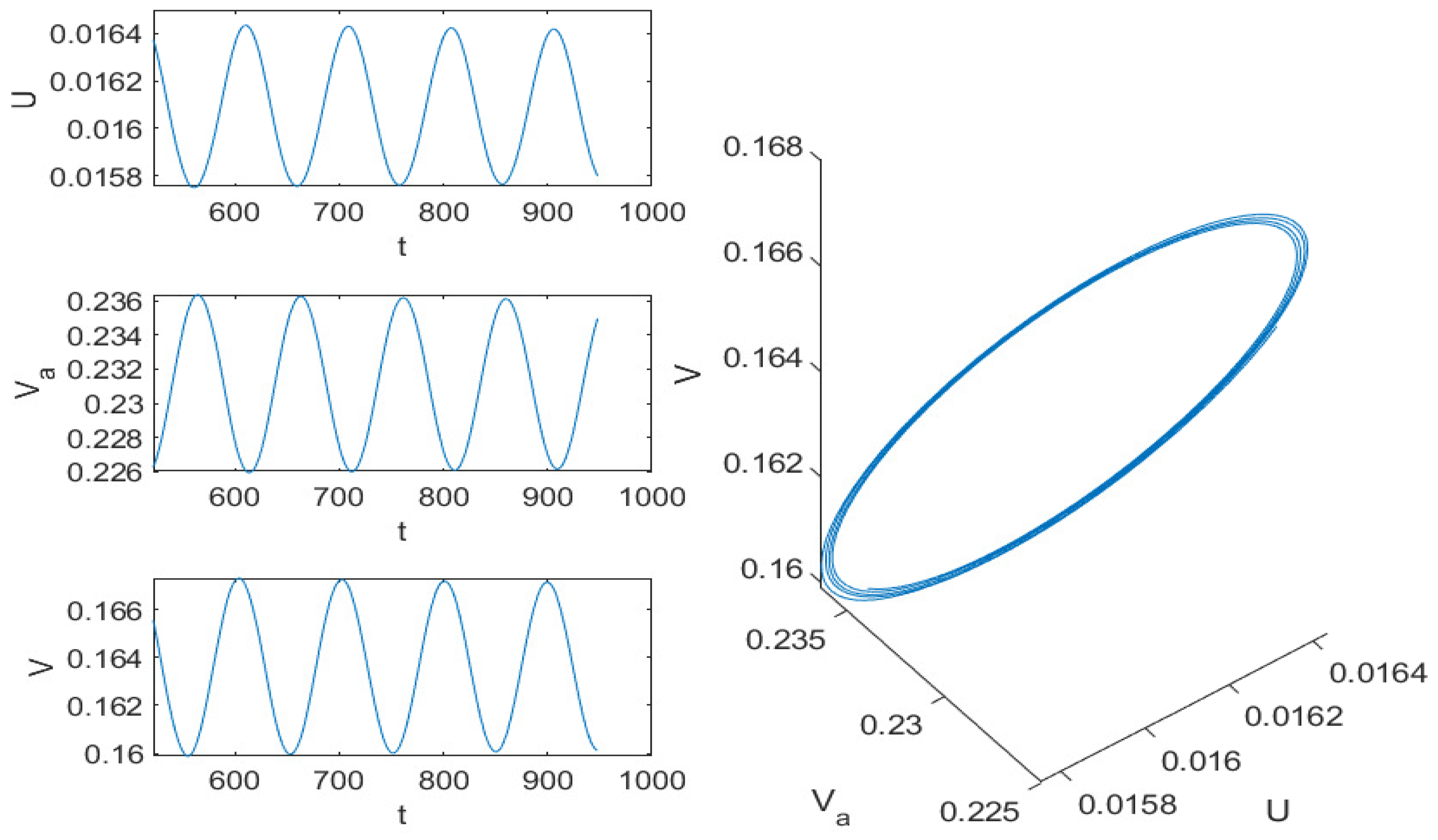
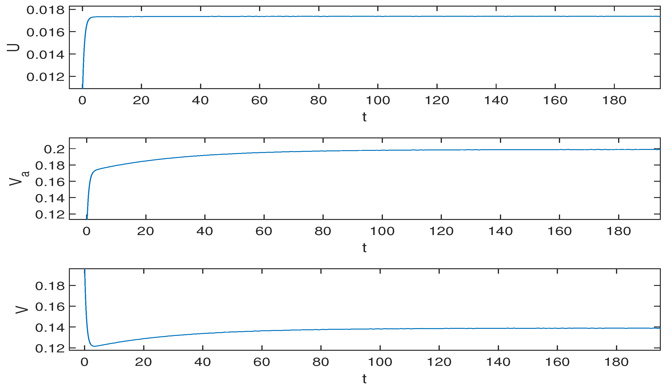
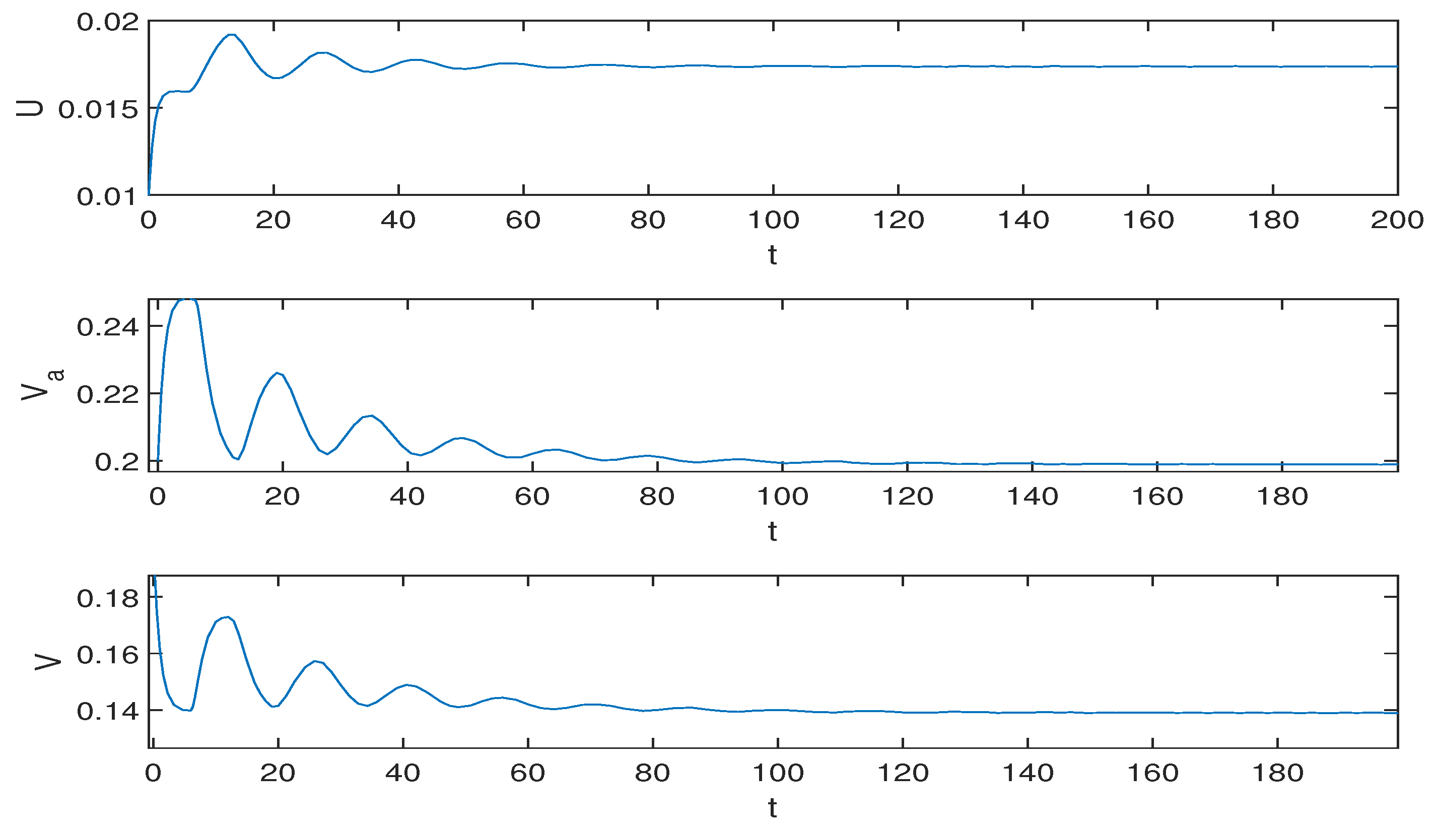
5.2. Numerical Simulation Results

In this section, we take the two groups of parameters given in Section 5.1 as examples for numerical simulations, and analyze the epidemic prevention and control effects in the sense of this group of parameters, and then provide a critical time ${\tau }_1^{\left(0\right)}$ for controllable widespread antibody failure, which provides a reference for the inoculation time of booster injection. In order to explore the effect of different epidemic prevention and control measures, we discuss the influence of fixed vaccination rate b, secondary vaccination rate $\alpha$ and failure rate $\gamma$ on the critical time ${\tau }_1^{\left(0\right)}$ of controllable widespread antibody failure. Finally, considering the frequent mutation of COVID-19 virus, we analyze the impact on epidemic prevention and control from the disease-related mortality rate c of the mutated strains.

For the first group parameters I:

$$B=0.0112, d=0.0069, c=0.04655, \gamma =0.675, a=0.49, b=0.5, \alpha =0.9.$$

Obviously, the assumption (H1) holds, system (1) only has one nonnegative equilibrium P. After calculation, the assumption (H2) holds. Thus, the equilibrium $P=(U^{*},V_a^{*},V^{*})$$\approx (0.016079,0.231125,0.163626)$ is locally asymptotically stable when $\tau =0$.

Using MATLAB, we can obtain ${\omega }_0=0.005233, Q_0\approx 0.225625, P_0\approx 0.947214, {\tau }_1^{\left(0\right)}\approx 38.2901$ by plugging parameters group I into Equations (6)–(8). According to Theorem 1, the equilibrium P is locally asymptotically stable at $\tau \in [0,{\tau }_1^{\left(0\right)})$, and the Hopf bifurcation occurs near the equilibrium P when $\tau ={\tau }_1^{\left(0\right)}$. Then, we obtain $\mathrm{Re}\left(K\right)>0, \mathrm{Re}\left(H\right)<0$ from Equations (17) and (21). Thus, according to Theorem 2, the system (1) has forward periodic solution and the bifurcating periodic solution is stable when ${\tau }_{\epsilon }>0$.

When $\tau$ = 0, we choose the initial value (0.02, 0.2, 0.2) and the equilibrium P of system (1) is locally asymptotically stable (see Figure 3).

When $\tau =6\in \left(0,{\tau }_1^{\left(0\right)}\right)$, we choose initial values $\left(0.015, 0.12, 0.2\right)$, and the equilibrium P of system (1) is locally asymptotically stable (see Figure 4).

When $\tau =38.4>{\tau }_1^{\left(0\right)}=38.2901$ is near ${\tau }_1^{\left(0\right)}$, we choose initial values $(0.012, 0.232, 0.162)$, and system (1) has stable forward periodic solution near the equilibrium P (see Figure 5).

It can be seen from Figure 3, Figure 4 and Figure 5, and the equilibrium P of system (1) is locally asymptotically stable when $\tau \in [0,{\tau }_1^{\left(0\right)})$ as shown in Figure 3 and Figure 4. The periodic solution of system (1) near equilibrium P is stable when $\tau$ is near ${\tau }_1^{\left(0\right)}$ as shown in Figure 5. The equilibrium P of system (1) is unstable when $\tau \in ({\tau }_1^{\left(0\right)},+\infty )$.

Remark 1.

Under the first group parameters I, it can be found by numerical simulations that the time $\tau =0$ of the wide range of antibody failure, that is, most people produce antibodies after vaccination and lose them in a short time. As the secondary vaccination rate α in the parameter is ideal, system (1) at this time is also stable, and the epidemic can be maintained even when the vaccine cost is high. When $\tau \in [0,{\tau }_1^{\left(0\right)})$, the shorter the time τ of the wide range of antibody failure is, the faster the antibody tends to stabilize, which also indicates that the number of secondary vaccinations is bigger, and the cost of controlling the epidemic is higher, but finally stabilizes near the equilibrium P. When $\tau >{\tau }_1^{\left(0\right)}$ is near ${\tau }_1^{\left(0\right)}$, the time τ of the wide range of antibody failure will change in a small range, and the antibody presence level will also show periodic changes. At this time, the epidemic prevention and control effect are controllable. When $\tau \in ({\tau }_1^{\left(0\right)},+\infty )$, the antibody distribution level cannot be controlled effectively. The fluctuation range of antibody distribution increases with the increase of time. According to the actual situation, the effectiveness of vaccines will have a certain period of time; generally, there is no permanent effective situation. Therefore, the time τ of a wide range of antibody failure is finite. Although there are periods when the antibody level is ideal, there are also periods when the antibody level is low. In this case, the antibody level cannot be controlled to be stable, and the low antibody level may lead to the outbreak of the epidemic, and the epidemic prevention and control effect are not ideal. Based on the above analysis, we can conclude that the optimal time ${\tau }_1^{\left(0\right)}=38.2901$ of controllable widespread antibody failure, which provides a reference for the second vaccination time of COVID-19 vaccine in medicine.

Next, we consider a group of parameters with higher mortality. In order to compare with the first group parameters I, we also idealize the secondary vaccination rate α, and select the secondary vaccination rate α under the future vaccination level. For the second group parameters $II$:

$$B=0.01231, d=0.01417, c=0.04655, \gamma =0.685, a=0.49, b=0.5, \alpha =0.92.$$

Obviously, the assumption  (H1)  holds, substituting these parameters values into Equation (2), we obtain that system (1) only has one nonnegative equilibrium $P=(U^{*},V_a^{*},V^{*})$$\approx (0.017375,$ $0.198918, 0.138938)$. After calculation, the assumption f̠(H2) holds. Thus, the equilibrium P is locally asymptotically stable when $\tau =0$.

When $\tau =0$, we choose the initial values $(0.01, 0.1, 0.2)$, and the equilibrium P of system (1) is locally asymptotically stable (see Figure 6).

Substituting these parameters’ values into Equation (7), we obtain $c_0\approx -0.000081, c1\approx 0.254617, c2\approx 1.033500$. By derivation of Equation (7), $\Delta \approx 1.217044, {\tilde{z}}_1\approx -0.505131, {\tilde{z}}_2\approx -0.872863$, we further calculate $h\left({\tilde{z}}_1\right)\approx 0.006119, h\left({\tilde{z}}_2\right)\approx -0.099943$. It satisfies assumption (H4). Using MATLAB, according to Equations (7) and (8), we obtain ${\omega }_1\approx 0.017865, Q_0\approx 0.62373, P_0\approx 0.78164, {\tau }_1^{\left(0\right)}\approx 35.2992$.

Thus, according to Theorem 1, the equilibrium P is locally asymptotically stable when $\tau \in [0,{\tau }_1^{\left(0\right)})$, and the Hopf bifurcation occurs near the equilibrium P when ${\tau }_1^{\left(0\right)}$. According to Equation (17), Equation (21), and Theorem 2, we conclude that $\mathrm{Re}\left(K\right)>0, \mathrm{Re}\left(H\right)<0$; thus, system (1) has a forward periodic solution and the bifurcating periodic solution is stable when ${\tau }_{\epsilon }>0$.

When $\tau =6\in [0,{\tau }_1^{\left(0\right)})$, we choose the initial value $(0.01, 0.2, 0.2)$, and the equilibrium P of system (1) is locally asymptotically stable (see Figure 7).

When $\tau =35.5>{\tau }_1^{\left(0\right)}=35.2992$, we choose the initial value $(0.01, 0.2, 0.15)$, the model (1) has a stable forward periodic solution near the equilibrium P (see Figure 8).

It can be seen from Figure 6, Figure 7 and Figure 8, the equilibrium P of system (1) is locally asymptotically stable as shown in Figure 6 and Figure 7. The equilibrium P of system (1) is unstable when $\tau \in ({\tau }_1^{\left(0\right)},+\infty )$. The equilibrium P of system (1) exhibits periodic fluctuation and bifurcates stable periodic solutions when $\tau$ approaches the critical time ${\tau }_1^{\left(0\right)}$ as shown in Figure 8. With the increase of $\tau$, the fluctuation tendency of the system (1) at the same time level also increases.

Remark 2.

According to the above numerical simulations, it can be found that, when the time $\tau <{\tau }_1^{\left(0\right)}$ of the wide range of antibody failure, it will eventually stabilize to the same antibody presence level after a certain time. According to our analysis, the smaller the time delay τ is, the faster it tends to be stable. However, according to the actual situation, the smaller the failure time is, the more total inoculated doses will increase, resulting in the increase of epidemic prevention cost, and ultimately maintain the same epidemic effect. Therefore, the ideal situation of epidemic prevention and control is that antibody levels are stable and controllable, the validity of vaccines is longer, and the cost of epidemic prevention can be saved and the cost of epidemic prevention can be reduced. When $\tau \in ({\tau }_1^{\left(0\right)},+\infty )$ and τ varies in a small range near ${\tau }_1^{\left(0\right)}$, the antibody levels will show periodic changes, but the overall situation of epidemic prevention and control is roughly stable. When $\tau >{\tau }_1^{\left(0\right)}$, the antibody presence level is high and low, and epidemic prevention and control is uncertain, which may lead to the outbreak of epidemic at the low antibody presence level.

Remark 3.

In the process of numerical simulations, we take the first group parameters I and the second group parameters II as examples and give the critical time ${\tau }_1^{\left(0\right)}$ of controllable widespread antibody failure of $38.5$ weeks and $35.3$ weeks, respectively, which can provide a reference for the vaccination time of COVID-19 vaccine booster injection in medical aspect to prolong the time of antibody disappearance.

Through the analysis of the simulations results of the two groups of parameters data, the antibody presence level is used to measure the epidemic prevention and control effect. Taking the time of six weeks of the wide range of antibody failure in the simulations as an example, the three groups population is roughly stable at $0.016, 0.231$, and $0.164$ (unit: million) for the first group parameters I, while the three groups population is stable at $0.017, 0.624$, and $0.139$ (unit: million) for the second group parameters II, and the proportions of antibody are $56.34\%$ and $56.21\%$, respectively. It can be concluded that, under the same epidemic vaccination strategy, the existence level of antibody is roughly the same, which is consistent with the reality.

In terms of the critical time ${\tau }_1^{\left(0\right)}$ for controllable widespread antibody failure, the group with lower mortality has better critical time ${\tau }_1^{\left(0\right)}$ for controllable widespread antibody failure than the group with higher mortality. The shorter the time $\tau$ of the wide range of antibody failure, the more vaccinations per person, the higher the cost of quarantine, and the greater the impact on normal life. Through the above theoretical analysis, we can know that the antibody existence level will be the same if the antibody failure time $\tau$ is appropriately increased within the critical time $\tau$ for controllable widespread antibody failure. Therefore, we can achieve the ideal of epidemic prevention and control through more effective and longer-lasting vaccines.

Next, we discuss the impact of different epidemic prevention and control strategies on the epidemic prevention and control. We use the combination of discrete and continuous variables to investigated the influence on the critical time ${\tau }_1^{\left(0\right)}$ of controllable widespread antibody failure. We will discuss the effects of validity factor a, fixed vaccination rate b, failure rate $\gamma$, and disease-related mortality c on the critical time ${\tau }_1^{\left(0\right)}$ in detail below. Finally, the impact of a sudden increase in disease-related mortality c and antibody failure rate $\gamma$ due to the emergence of a mutant strain of COVID-19 is analyzed.

We first analyze the impact factor a on vaccine effectiveness on the vaccination rate, and thus affect the critical time ${\tau }_1^{\left(0\right)}$ of controllable widespread antibody failure in system (1), and add the secondary vaccination rate $\alpha$ of a discrete case as shown in Figure 9:

In Figure 9, it observes that the increase of influence factor a has a significant promoting effect on the critical time ${\tau }_1^{\left(0\right)}$, and the promoting relationship between them is approximately linear. Therefore, in the context of this discussion, we can promote the safety and effectiveness of COVID-19 vaccines by strengthening publicity, so as to improve the impact of vaccine effectiveness on vaccination, which also provides some suggestions for future epidemic prevention and control.

When other parameters are fixed, the influence of fixed vaccination rate b in the continuous case and secondary vaccination rate $\alpha$ in the discrete case on the critical time ${\tau }_1^{\left(0\right)}$ is investigated in Figure 10.

In Figure 10, we find that the critical time ${\tau }_1^{\left(0\right)}$ will be suppressed by fixed vaccination rate b in a linear manner. In comparison with Figure 9, in order to increase the vaccination rate of COVID-19, to improve the final antibody presence level, and to promote the critical time ${\tau }_1^{\left(0\right)}$, we should properly regulate the vaccination strategy from two aspects: on the one hand, we should appropriately improve the role of effectiveness in vaccination willingness; on the other hand, the fixed vaccination rate b brought about by other factors should be appropriately reduced.

As the COVID-19 virus continues to mutate, it has created multiple mutated strains with higher transmissibility and mortality. Then, we consider the effects of the failure rate $\gamma$ (see Figure 11) and mortality rate c (see Figure 12) on the critical time ${\tau }_1^{\left(0\right)}$.

From Figure 11, it can be concluded that the smaller the antibody failure rate $\gamma$ is, the larger the critical time ${\tau }_1^{\left(0\right)}$ is. The influence of failure rate $\gamma$ on the critical time ${\tau }_1^{\left(0\right)}$ decreases with the increase of failure rate $\gamma$. When the failure rate $\gamma >0.68$, the effect of $\gamma$ on ${\tau }_1^{\left(0\right)}$ is almost zero. When the failure rate $\gamma <0.68$, the smaller $\gamma$ is, the more obvious the effect of increasing the critical time ${\tau }_1^{\left(0\right)}$ is. Therefore, from the perspective of epidemic control, we have confirmed the need to reduce the vaccine’s own failure rate $\gamma$ from the perspective of epidemic control.

In the case of the COVID-19 mutant strains, the mutant strains cause a spike in antibody failure rate $\gamma$. If the failure rate $\gamma$ of the primary antibody is less than $0.68$, the $\gamma$ surge will cause the shortening of the critical time ${\tau }_1^{\left(0\right)}$. If the failure rate $\gamma$ of the original antibody is high, the effect of $\gamma$ surge may be relatively small. Therefore, we should keep $\tau$ at a distance ${\tau }_1^{\left(0\right)}$ to prevent the risk of uncertainty due to mutant strains.

From Figure 12, comparing the influence of disease mortality rate c and secondary vaccination rate $\alpha$ on the critical time ${\tau }_1^{\left(0\right)}$, we can find that the influence of disease mortality rate c on the critical time ${\tau }_1^{\left(0\right)}$ is significantly higher than that of secondary vaccination rate $\alpha$ on the critical time ${\tau }_1^{\left(0\right)}$.

From the perspective of the COVID-19 mutant strains, the COVID-19 mutant strains may cause discrete changes in disease mortality rate c. We consider the effect of the discrete change of c on ${\tau }_1^{\left(0\right)}$ in Figure 12. Small changes in disease mortality rate c caused by the mutated strains may lead to large changes in the critical time ${\tau }_1^{\left(0\right)}$ of controllable widespread antibody failure, leading to instability in the vaccination system. After a certain period of time, antibody levels rise and fall, and the COVID-19 mutated strains may trigger a new outbreak. Therefore, we should pay attention to the variation trend of mutant strains and change the inoculation strategy in time when necessary. Before it becomes a mainstream mutant strain, countermeasures should be taken to ensure the effect of epidemic prevention and control.

Remark 4.

According to Figure 9, Figure 10, Figure 11 and Figure 12, we find that the secondary vaccination rate α has a turning point ${\alpha }_0$ around $0.91$. In a certain range before ${\alpha }_0$, as shown in Figure 9 and Figure 10, the increase of the secondary vaccination rate α leads to the decrease of the critical time ${\tau }_1^{\left(0\right)}$, and the closer it is to $0.91$, the less the effect is. In a certain range after ${\alpha }_0$, the increase of secondary vaccination rate α will increase the critical time ${\tau }_1^{\left(0\right)}$, and the change relationship between the two is approximately linear, as shown in Figure 11 and Figure 12.

6. Conclusions

In this paper, an $U{V}_{a}V$ vaccination model with time-delay was constructed for COVID-19 vaccination based on the transmission characteristics of COVID-19 vaccine antibodies. Compared with the traditional SIR model, this paper paid more attention to the presence of antibodies in the population and the vaccination situation of vaccines. At the same time, the effect of vaccination intention on vaccination rate was added into the model. We also analyzed the existence and stability of equilibrium, and studied the existence and stability of the Hopf bifurcation associated with existing equilibrium. Then, we derived the normal form of the Hopf bifurcation in the vaccination model by using the multiple time scales method. Finally, according to the parameters estimations and the data given in the literature, it was divided into two groups of parameters. One group is the small natural mortality parameters, and the other is the natural mortality parameters. Numerical simulations were carried out to verify the correctness of the theoretical analysis.

In [40], Lu et al. studied the impact of critical treatment time on epidemic prevention and control. In this paper, we considered the impact of the large-scale failure time of critical antibodies on epidemic prevention and control from the perspective of failure time. Numerical simulations showed that, when the time $\tau <{\tau }_1^{\left(0\right)}$ of the wide range of antibody failure was obtained in the sense of two parameters, after a certain time, the antibody would eventually approach the same level of existence, and the epidemic prevention and control effects were basically the same. Different failure time $\tau$ would produce different critical time ${\tau }_1^{\left(0\right)}$; the shorter the failure time $\tau$, the faster the critical time ${\tau }_1^{\left(0\right)}$. However, the shorter the lapse, the greater the total number of vaccinations. Obviously, on the one hand, frequent vaccination would inevitably bring a great impact on people’s life and work, but also seriously hindered the development of society and the country; on the other hand, frequent vaccinations increased the cost of prevention. When $\tau$ changed in a small range near ${\tau }_1^{\left(0\right)}$, we believed that the antibody level changed periodically and the epidemic prevention and control situation was under control. When $\tau >{\tau }_1^{\left(0\right)}$, the antibody presence level was high and low, and there was a risk of causing a new epidemic. Therefore, taking these two groups of parameters as examples, we gave the critical time ${\tau }_1^{\left(0\right)}$ of controllable widespread antibody failure of $38.5$ weeks and $35.3$ weeks, respectively, and the stability of the system would be greatly affected before and after the critical time ${\tau }_1^{\left(0\right)}$. This provided a medical reference for the time of COVID-19 vaccine booster injection to prolong the time of antibody disappearance.

In addition, according to Wang’s et al. [41] research, the protection rate, the infection rate, and the average quarantine time had a significant impact on the prevention and the control of the epidemic. We discussed the impact of different vaccination strategies on the time ${\tau }_1^{\left(0\right)}$ for controllable widespread antibody failure, and considered the influence of COVID-19 mutated strains on epidemic prevention and control. We also provided some suggestions for epidemic prevention and control from the perspective of mathematical model and dynamic property analysis as follows:

(1): In the positive feedback mechanism, the effect factor a on vaccine effectiveness had a significant promoting effect on the critical time ${\tau }_1^{\left(0\right)}$. We can increase the impact of vaccine effectiveness on vaccination by increasing awareness about the safety and effectiveness of COVID-19 vaccines.

(2): In the positive feedback mechanism, the relatively fixed vaccination rate b inhibited the critical time ${\tau }_1^{\left(0\right)}$. Combined with (1), vaccination strategies were appropriately regulated from two aspects: on the one hand, the role of effectiveness in vaccination intention was appropriately increased; on the other hand, the fixed vaccination rate b brought about by other factors should be appropriately reduced.

(3): Considered that the mutant strains of COVID-19 may cause a sudden increase in the antibody failure rate $\gamma$ and thus reduced the critical time ${\tau }_1^{\left(0\right)}$. In addition, the smaller the failure rate $\gamma$ is, the more obvious the effect of critical time is. Therefore, from the perspective of model sensitivity, we confirmed the necessity of reducing vaccine failure rate $\gamma$.

(4): Considered that mutated strains of COVID-19 may caused mutations in disease-related mortality c. A small change in disease-related mortality c may cause a large change in the critical time ${\tau }_1^{\left(0\right)}$, which may change the system (1) stability. We should pay attention to the variation trend of mutant strains and change the inoculation strategy in time when necessary. Before the mutated strains cause a new outbreak, analysis showed that we can take measures such as vaccination boosters to reduce vaccine failure rates, thus reducing mortality due to disease and ensuring that the outbreak is within manageable limits.

References

1. Maramattom, B.V.; Bhattacharjee, S. Neurological complications with COVID-19: A contemporaneous review. Ann. Indian Acad. 2020, 23, 468–476. [Google Scholar] [CrossRef] [PubMed]
2. Zhao, D.H.; Lin, H.J.; Zhang, Z.R. Evidence-based framework and implementation of China’s strategy in combating COVID-19. Risk Manag. Healthc. Policy 2020, 13, 1989–1998. [Google Scholar] [CrossRef] [PubMed]
3. Atalan, A. Is the lockdown important to prevent the COVID-19 pandemic? Effects on psychology, environment and economy-perspective. Ann. Med. Surg. 2012, 56, 38–42. [Google Scholar] [CrossRef] [PubMed]
4. Acharya, S.R.; Moon, D.H.; Shin, Y.C. Assessing attitude toward COVID-19 vaccination in South Korea. Front. Psychol. 2021, 12, 694151. [Google Scholar] [CrossRef] [PubMed]
5. Chakraborty, C.; Sharma, A.R.; Bhattacharya, M.; Agoramoorthy, G.; Lee, S.S. Asian-origin approved COVID-19 vaccines and current status of COVID-19 vaccination program in Asia: A critical analysis. Vaccines 2021, 9, 600. [Google Scholar] [CrossRef]
6. Tagoe, E.T.; Sheikh, N.; Morton, A.; Nonvignon, J.; Sarker, A.R.; Williams, L.; Megiddo, I. COVID-19 vaccination in lower-middle income countries: National stakeholder views on challenges, barriers and potential solutions. Front. Public Health 2021, 9, 709127. [Google Scholar] [CrossRef]
7. Van De Pas, R.; Van De Pas, M.A.; Ravinetto, R.; Srinivas, P.; Ochoa, T.J. COVID-19 vaccine equity: A health systems and policy perspective. Expert Rev. Vaccines 2021, 21, 25–36. [Google Scholar] [CrossRef]
8. Zhu, F.; Li, Y.; Guan, X.; Hou, L.; Wang, W.; Li, J.X.; Wu, S.P.; Wang, B.S.; Wang, Z.; Wang, L.; et al. Safety, tolerability and immunogenicity of a recombinant adenovirus type-5 vectored COVID-19 vaccine: A dose-escalation, open-label, non-randomised, first-in-human trial. Lancet 2020, 395, 1845–1854. [Google Scholar] [CrossRef]
9. Zhu, Y.; Wei, Y.; Sun, C.; He, H. Development of vaccines against COVID-19. Prev. Med. 2021, 33, 143–148. [Google Scholar]
10. Hodgson, S.H.; Mansatta, K.; Mallett, G.; Harris, V.; Emary, K.R.W.; Pollard, A.J. What defines an efficacious COVID-19 vaccine? A review of the challenges assessing the clinical efficacy of vaccines against SARS-CoV-2. Lancet Infect. Dis. 2021, 21, E26–E35. [Google Scholar] [CrossRef]
11. Grubaugh, N.D.; Hanage, W.P.; Rasmussen, A.L. Making sense of mutation: What D614G means for the COVID-19 pandemic remains unclear. Cell 2020, 182, 794–795. [Google Scholar] [CrossRef] [PubMed]
12. Olaniyi, S.; Obabiyi, O.S.; Okosun, K.O.; Oladipo, A.T.; Adewale, S.O. Mathematical modelling and optimal cost-effective control of COVID-19 transmission dynamics. Eur. Phys. J. Plus 2020, 135, 938. [Google Scholar] [CrossRef] [PubMed]
13. Abdy, M.; Side, S.; Annas, S.; Nur, W.; Sanusi, W. A SIR epidemic model for COVID-19 spread with fuzzy parameter: The case of Indonesia. Adv. Differ. Equ. 2021, 2021, 105. [Google Scholar] [CrossRef] [PubMed]
14. Bardina, X.; Ferrante, M.; Rovira, C. A stochastic epidemic model of COVID-19 disease. Aims Math. 2020, 5, 7661–7677. [Google Scholar] [CrossRef]
15. He, S.B.; Peng, Y.X.; Sun, K.H. SEIR modeling of the COVID-19 and its dynamics. Nonlinear Dynam. 2020, 101, 1667–1680. [Google Scholar] [CrossRef] [PubMed]
16. Algehyne, E.A.; Din, R.U. On global dynamics of COVID-19 by using SQIR type model under nonlinear saturated incidence rate. Alex. Eng. J. 2021, 60, 393–399. [Google Scholar] [CrossRef]
17. Li, N.; Wang, Z.Y.; Pei, Z. Sequential resource planning decisions in an epidemic based on an innovative spread model. IEEE T. Autom. Sci. Eng. 2022, 19, 677–691. [Google Scholar] [CrossRef]
18. Li, M.Y.; Zhang, Y.J.; Zhou, X.H. Analysis of transimission pattern of COVID-19 based on EM algorithm and epidemiological data. Acta Math. Appl. Sin. 2020, 43, 427–439. [Google Scholar]
19. Chong, P.Y.; Yin, H. System dynamics simulation on spread of COVID-19 by traffic and transportation. J. Traf. Trans. Eng. 2020, 20, 100–109. [Google Scholar]
20. Cadoni, M.; Gaeta, G. Size and timescale of epidemics in the SIR framework. Phys. D 2020, 411, 132626. [Google Scholar] [CrossRef]
21. Yang, L.L.; Su, Y.M.; Zhuo, X.J. Comparison of two different types of fractional-order COVID-19 distributed time-delay models with real data application. Int. J. Mod. Phys. B 2021, 35, 2150219. [Google Scholar] [CrossRef]
22. Radha, M.; Radha, S. A study on COVID-19 transmission dynamics: Stability analysis of SEIR model with Hopf bifurcation for effect of time delay. Adv. Differ. Equ. 2020, 1, 523. [Google Scholar] [CrossRef] [PubMed]
23. Chang, X.H.; Wang, J.R.; Liu, M.X.; Jin, Z.; Han, D. Study on an SIHRS model of COVID-19 pandemic with impulse and time delay under media coverage. IEEE Access 2021, 9, 49387–49397. [Google Scholar] [CrossRef] [PubMed]
24. Zhu, C.C.; Zhu, J. Dynamic analysis of a delayed COVID-19 epidemic with home quarantine in temporal-spatial heterogeneous via global exponential attractor method. Chaos Solitons Fract. 2021, 143, 110546. [Google Scholar] [CrossRef] [PubMed]
25. Yang, F.F.; Zhang, Z.Z. A time-delay COVID-19 propagation model considering supply chain transmission and hierarchical quarantine rate. Adv. Differ. Equ. 2021, 1, 191. [Google Scholar] [CrossRef]
26. Hossain, M.K.; Hassanzadeganroudsari, M.; Apostolopoulos, V. The emergence of new strains of SARS-CoV-2. What does it mean for COVID-19 vaccines? Expert Rev. Vaccines 2021, 20, 635–638. [Google Scholar] [CrossRef]
27. Tartof, S.Y.; Slezak, J.M.; Fischer, H.; Hong, V.; Ackerson, B.K.; Ranasinghe, O.N.; Frankland, T.B.; Ogun, O.A.; Zamparo, J.M.; Gray, S.; et al. Effectiveness of mRNA BNT162b2 COVID-19 vaccine up to 6 months in a large integrated health system in the USA: A retrospective cohort study. Lancet 2021, 398, 1407–1416. [Google Scholar] [CrossRef]
28. Jara, A.; Undurraga, E.A.; Gonzalez, C.; Paredes, F.; Fontecilla, T.; Jara, G.; Pizarro, A.; Acevedo, J.; Leo, K.; Leon, F.; et al. Effectiveness of an inactivated SARS-CoV-2 vaccine in Chile. N. Engl. J. Med. 2021, 385, 875–884. [Google Scholar] [CrossRef]
29. Xiao, L.L.; Zhang, Y.; Hu, X.W.; Liu, T.; Liu, Y. Analysis of global prevalence of SARS-CoV-2 varia. Chin. J. Front. Health Quar. 2022, 45, 10–12. [Google Scholar]
30. Shi, Q.F.; Gao, X.D.; Hu, B.J. Research progress on characteristics, epidemiology and control measure of SARS-CoV-2 delta voc. Chin. J. Nosocomiol. 2021, 31, 3703–3707. [Google Scholar]
31. Raman, R.; Patel, K.; Ran, K. COVID-19: Unmasking emerging SARS-CoV-2 variants, vaccines and therapeutic strategies. Biomolecules 2021, 11, 993. [Google Scholar] [CrossRef] [PubMed]
32. Darvishi, M.; Rahimi, F.; Talebi, B.A. SARS-CoV-2 lambda (C.37): An emerging variant of concern. Gene. Rep. 2021, 25, 101378. [Google Scholar] [CrossRef] [PubMed]
33. Choi, J.Y.; Smith, D.M. SARS-CoV-2 variants of concern. Yonsei Med. J. 2021, 62, 961–968. [Google Scholar] [CrossRef] [PubMed]
34. Mohapatra, R.K.; Tiwari, R.; Sarangi, A.K.; Sharma, S.K.; Khandia, R. Twin combination of omicron and delta variants triggering a tsunami wave of ever high surges in COVID-19 cases: A challenging global threat with a special focus on the Indian subcontinent. J. Med. Virol. 2022, 94, 1761–1765. [Google Scholar] [CrossRef] [PubMed]
35. Zhao, X.H.; Ning, Y.L.; Chen, M.I.C.; Cook, A.R. Individual and population trajectories of influenza antibody titers over multiple seasons in a tropical country. Am. J. Epidemiol. 2018, 187, 135–143. [Google Scholar] [CrossRef] [PubMed]
36. Ibarrondo, F.J.; Fulcher, J.A.; Yang, O.O. Rapid decay of Anti-SARS-CoV-2 antibodies in persons with mild COVID-19. N. Engl. J. Med. 2020, 383, 1085–1087. [Google Scholar] [CrossRef] [PubMed]
37. Li, J.; Ao, N.; Yin, J.H. Willingness for COVID-19 vaccination and its influencing factors among outpatient clinic attendees in Kunming city. China J. Public Health 2021, 37, 411–414. [Google Scholar]
38. Sarwar, A.; Nazar, N.; Nazar, N.; Qadir, A. Measuring vaccination willingness in response to COVID-19 using a multi-criteria-decision-making method. Hum. Vaccines 2021, 17, 1–8. [Google Scholar] [CrossRef]
39. Liu, R.G.; Liu, Y.X.; Nicholas, S.; Leng, A.L.; Maitland, E.; Wang, J. COVID-19 vaccination willingness among Chinese adults under the free vaccination policy. Vaccines 2021, 9, 292. [Google Scholar] [CrossRef]
40. Lu, H.f.; Ding, Y.T.; Gong, S.L.; Wang, S.S. Mathematical modeling and dynamic analysis of SIQR model with delay for pandemic COVID-19. Math. Biosci. Eng. 2021, 18, 3197–3214. [Google Scholar] [CrossRef]
41. Wang, J.W.; Cui, Z.W.; Dong, S. Simulation of COVID-19 propagation and transmission mechanism and intervention effect based on generalized SEIR model. Sci. Technol. Rev. 2020, 38, 130–138. [Google Scholar]
Figure 1. Flow chart for the U V a V model.
Mathematics 10 01583 g001
Figure 2. Annual natural mortality d in a low mortality country.
Mathematics 10 01583 g002
Figure 3. When τ = 0, the equilibrium P of system (1) is locally asymptotically stable.
Mathematics 10 01583 g003
Figure 4. When τ = 4 , the equilibrium P of system (1) is locally asymptotically stable.
Mathematics 10 01583 g004
Figure 5. When τ = 38.4 , the periodic solution of system (1) near equilibrium P is stable.
Mathematics 10 01583 g005
Figure 6. When τ = 0, the equilibrium P of system (1) is locally asymptotically stable.
Mathematics 10 01583 g006
Figure 7. When τ = 6 , the equilibrium P of system (1) is locally asymptotically stable.
Mathematics 10 01583 g007
Figure 8. When τ = 35.5 , the periodic solution of system (1) near equilibrium P is stable.
Mathematics 10 01583 g008
Figure 9. The influence of positive feedback factor a on the critical time τ 1 ( 0 ) .
Mathematics 10 01583 g009
Figure 10. Influence of fixed vaccination rate b (continuous case) and secondary vaccination rate α (discrete case) on the critical time τ 1 ( 0 ) .
Mathematics 10 01583 g010
Figure 11. The influence of continuous antibody failure rate γ and discrete secondary vaccination rate α on the critical time τ 1 ( 0 ) .
Mathematics 10 01583 g011
Figure 12. The influence of continuous secondary vaccination rate α and discrete mortality rate c on the critical time τ 1 ( 0 ) .
Mathematics 10 01583 g012