Steady Flow of Burgers’ Nanofluids over a Permeable Stretching/Shrinking Surface with Heat Source/Sink

Abstract

An engineered fluid, called nanofluid, is expected to have better thermal conductivity than conventional working fluids. The superior heat transfer performance and various possible applications promote the analysis of nanofluids in different flow geometries. This paper studies the flow of non-Newtonian Burgers’ nanofluids over a permeable stretching/shrinking surface with a heat source/sink. In the current study, we highlight the use of the single-phase nanofluid model in studying the boundary layer flow. The basic partial differential equations are transformed into ordinary (similarity) differential equations. Then, the resulting equations and boundary conditions are solved numerically in MATLAB using the bvp4c package. Triple solutions are presented, and stability analysis certifies that the first solution is physically realizable in practice. It is found that the increment of the heat source parameter raised the temperature profile of the nanofluids. Al₂O₃/H₂O and Cu/H₂O nanofluids produced the highest skin friction coefficient in the flow over stretching and shrinking surfaces, respectively. Meanwhile, Cu/H₂O nanofluid showed a better heat transfer performance when compared to Al₂O₃/H₂O and TiO₂/H₂O nanofluids. The present study is novel and could serve as a reference to other researchers for further analysis of heat transfer performance and the rheological behavior of nanofluids.

1. Introduction

Every fluid that obeys Newton’s law of viscosity, i.e., viscosity is independent of shear stress, is termed a Newtonian fluid. Meanwhile, fluids such as toothpaste, ketchup, polymers, colloids, and tars with variable viscosity depending on the shear rate and shear stress are called non-Newtonian fluids. The non-Newtonian fluids are further classified into three sub-categories: the differential-type, integral-type, and rate-type. Fluid models such as Maxwell, Oldroyd-B, and Burgers are proposed to represent the rate-type fluids, characterized by the fluid relaxation and retardation time phenomena [1]. Among these models, only the Burgers’ fluid model expresses relaxation and retardation time properties simultaneously, which is suitable for describing the rheological properties of assorted viscoelastic materials; for example, asphalt, soil, cheese, and polymeric liquids (see Hayat et al. [2]; Rashidi et al. [3]). However, the Burgers’ model is less popular among researchers due to its complex constitutive equations and mathematical formulation. Some of the studies on Burgers’ fluid are those by Alsaedi et al. [4], Hayat et al. [5,6,7,8], Ahmad et al. [9], Khan et al. [10], Imran et al. [11], Safdar et al. [12], Akram et al. [13], Jiang et al. [14], and Gangadhar et al. [15].

Rapid development in engineering applications and electronic devices demands a more efficient and advanced nanofluid to act as a coolant in removing excess heat from devices. Nanofluids are defined by Choi [16] as fluids containing particles with an average size of 10 nanometers (e.g., carbon nanotubes, carbides, metals, and oxides). These particles are dispersed in a conventional heat transfer fluid (e.g., water, oil, and ethylene glycol), called base fluid. The synthesis of nanofluids serves the purpose of finding superior heat transfer fluid with better performance than conventional fluids. Incorporating high thermal conductivity nanoparticles into the conventional fluids improves the heat transfer performance of the fluids (see Alghamdi [17]; Khan and Alzahrani [18]; Hayat et al. [19,20]; Iqbal et al. [21]). The processes of preparing nanofluids were elucidated by Xuan and Li [22], Das et al. [23], and Khattak et al. [24]. Due to various applications of nanofluids, for example, in manufacturing processes, microelectronics, biomedical field, food processing, nuclear cooling system, and computer processor, it is interesting to study the flow of different nanofluids over diverse physical geometries and conditions. It is worth mentioning that references to nanofluids can be found in the books by Das et al. [25], Nield and Bejan [26], Minkowycz et al. [27], and Shenoy et al. [28], and in the review papers by Manca et al. [29], Myers et al. [30], Mahian et al. [31,32,33], and others. Khan and Khan [34] discussed the forced convection flow of Burgers’ nanofluid over a stretching sheet. Whereas Khan and Khan [35] studied the free convection flow of Burgers’ nanofluid in the presence of heat generation/absorption. The effects of the heat generation parameter on the temperature profile were the opposite of the heat absorption parameter. Then, Hayat et al. [19] analyzed the flow of Burgers’ nanofluid with convective boundary condition and a magnetic field. The nanofluid velocity in hydromagnetic flow was shown to be slower than in the hydrodynamic flow due to the existence of Lorentz force. Meanwhile, the relaxation and retardation time parameters reduce and enhance the velocity of the nanofluid, respectively. The same results were reported by Hayat et al. [20] for mixed convection flow. The Buongiorno nanofluid model [36] was utilized in [19,20,34,35] with thermophoresis and Brownian motion considered in these studies. Rashidi et al. [3] found that the thermophoresis and Brownian motion parameters improve the molecular movement that raises the nanofluid temperature. However, the nanofluid concentration decreases with the increment of the Brownian motion parameter. The semi-analytical solution for Burgers’ nanofluid flow between parallel channels was presented by Muhammad et al. [37]. Meanwhile, the study by Khan et al. [38] and Khan et al. [1] revealed that the enhancement of thermal and concentration boundary layers was achieved through the increase of Burgers’ material parameter. However, the augmentation of this parameter impedes the nanofluid velocity. Other recent studies on Burgers’ nanofluid were carried out by Iqbal et al. [21], Khan et al. [39], Waqas et al. [40], Ramzan et al. [41], and Wang et al. [42].

The present study will combine the Burgers’ fluid model and the single-phase Tiwari and Das [43] nanofluid model to depict the flow of nanofluids over a stretching/shrinking surface with heat generation/absorption. Flow with such geometry and conditions may have applications for heat exchangers, cooling of devices, nuclear reactors, automobiles, extrusion of plastic sheets, and many others. A previous study on Burgers’ nanofluid, conducted by Khan and Khan [35], adopted the two-phase Buongiorno nanofluid model and only analyzed the stretching sheet case. Contrary to the Buongiorno model, the Tiwari and Das model considers the effects of nanoparticles volume fraction with the assumption of a no-slip condition between the nanoparticles and base fluid. The non-linear ordinary differential equations and boundary conditions will be solved numerically in MATLAB using the bvp4c package. The results, presented in tables and graphs, will be examined and discussed in detail. Through the authors’ knowledge, studies on Burgers’ fluid using the single-phase nanofluid model have not been carried out by other researchers. Thus, the current study is an original work to be added to the limited literature and provides new information to the researchers working in the area of nanofluids. Three different nanofluids are considered, namely Cu/H₂O, Al₂O₃/H₂O, and TiO₂/H₂O. It should be mentioned that we are able to generate triple solutions for the shrinking case ($\lambda <0)$, which doesn’t exist for many shrinking problems.

2. Mathematical Model

Consider the steady flow of Burgers’ fluid over a permeable stretching/shrinking surface (sheet) with heat source/sink, as shown in Figure 1. $x$ and $y$ are the Cartesian coordinates such that the $x$−axis runs along the surface of the sheet while the $y$−axis is in the normal direction to the sheet with the flow being at $y\ge 0$. As a thermal enhancement, three different nanoparticles, namely Cu, Al₂O₃, and TiO₂, are diluted in a base fluid (water). Assumptions are made such that the velocity of the stretching/shrinking sheet is $U_w\left(x\right)$, and the mass transfer is $v_w$ with $v_w<0$ for suction and $v_w>0$ for injection. The temperature of the sheet is constant $T_w$, while the working fluid temperature is $T_{\infty }$.

The equations governing the steady boundary layer flow of an incompressible Burgers’ nanofluid with a heat source/sink are written in Cartesian coordinates $\left(x,y\right)$ as (see Khan and Khan [35]; Ejaz et al. [45]):

$$\frac{\partial u }{\partial x}+\frac{\partial v }{\partial y}=0,$$

(1)

$$\begin{array}{c}u \frac{\partial u}{\partial x}+v \frac{\partial u}{\partial y}+{\lambda }_1\left(v^2 \frac{{\partial }^{2}u}{\partial y^2}+2 u v \frac{{\partial }^{2}u}{\partial x \partial y}\right)+\\ {\lambda }_2[v^3\frac{{\partial }^{3}u}{\partial y^3}+3 v^2\left(\frac{\partial v}{\partial y} \frac{{\partial }^{2}u}{\partial y^2}+\frac{\partial u}{\partial y} \frac{{\partial }^{2}u}{\partial x \partial y}\right)+3 u v^2\frac{{\partial }^{3 }u}{\partial x \partial y^2}+\\ 2 uv \frac{\partial v}{\partial y} \frac{{\partial }^{2}u}{\partial x \partial y}]= \frac{{\mu }_n}{{\rho }_n} \left[\begin{array}{c}\frac{{\partial }^{2}u}{\partial y^2}+{\lambda }_3 (u \frac{{\partial }^{3}u}{\partial x \partial y^2}+v \frac{{\partial }^{3}u}{\partial y^3}-\\ \frac{\partial u}{\partial x} \frac{{\partial }^{2}u}{\partial y^2}-\frac{\partial u}{\partial y} \frac{{\partial }^{2}v}{\partial y^2})\end{array}\right],\end{array}\}$$

(2)

$$u \frac{\partial T}{\partial x}+v \frac{\partial T}{\partial y}=\frac{k_n}{{\left(\rho C_p\right)}_n} \frac{{\partial }^{2}T}{\partial y^2}+\frac{Q}{{\left(\rho C_p\right)}_n} \left(T-T_{\infty }\right),$$

(3)

along with the boundary conditions (see Hayat et al. [7])

$$\begin{array}{}\\ \begin{array}{c}v=v_w,\hspace{1em}u=U_w\left(x\right) \lambda =a x \lambda ,\hspace{1em}T=T_w\hspace{1em}\mathrm{at}\hspace{1em}y=0\end{array}\\ u\to 0,\hspace{1em}\frac{\partial u}{\partial y}\to 0,\hspace{1em}T\to T_{\infty }\hspace{1em}as\hspace{1em}y\to \infty .\end{array},\}$$

(4)

Here, $u$ and $v$ represent the velocity components along $x-$ and $y-$axes, $a$ is a positive constant, $T$ is the temperature, ${\lambda }_1$ and ${\lambda }_3 \left(\le {\lambda }_1\right)$ are the relaxation and retardation times, respectively, ${\lambda }_2$ is the material parameter of the Burgers’ fluid, $Q_0$ is the heat generation/absorption parameter, and $\lambda$ is the constant stretching/shrinking parameter with $\lambda <0$ for the shrinking sheet, $\lambda =0$ for static sheet, and $\lambda >0$ for the stretching sheet.

Next, ${\rho }_n$ is the density, ${\left(\rho C_p\right)}_n$ is the heat capacity, ${\mu }_n$ is the dynamic viscosity, and $k_n$ is the thermal conductivity of the nanofluid, given by (see Ho et al. [46]; Sheremet et al. [47]):

$$\begin{array}{c}{\rho }_n=\left(1-\varphi \right) {\rho }_f+\varphi {\rho }_s,\\ {\left(\rho C_p\right)}_n=\left(1-\varphi \right) {\left(\rho C_p\right)}_f+\varphi {\left(\rho C_p\right)}_s,\\ \frac{{\mu }_n}{{\mu }_f}=\frac{1}{{\left(1-\varphi \right)}^{2.5}},\\ \frac{k_n}{k_f}=\frac{k_s+2k_f-2\varphi \left(k_f-k_s\right)}{k_s+2k_f+2\varphi \left(k_f-k_s\right)}.\end{array}\}$$

(5)

Here, the suffixes $f,n,\mathrm{and}s$ describe the base fluid, nanofluid, and nanoparticle, respectively, $\varphi$ is the nanoparticle volume fraction $\left(\varphi =0\mathrm{correspond}\mathrm{to}\mathrm{a}\mathrm{regular}\mathrm{fluid}\right)$, and $C_p$ is the heat capacity at constant pressure.

Table 1. Thermal and physical characteristics for nanoparticles (see Oztop and Abu Nada [48]).

Properties	$\mathit{\rho } ($kg/m3)	${\mathit{C}}_{\mathit{p}} (\mathbf{J}\mathbf{/}\mathbf{kg}\mathbf{K}\mathbf{)}$	$\mathit{k} \mathbf{(}\mathbf{W}\mathbf{/}\mathbf{m}\mathbf{K}\mathbf{)}$	$\mathit{P}\mathit{r}$
Cu	8933	385	400	-
Al2O3	3970	765	40	-
TiO2	4250	686.2	8.9538	-
H2O	997.1	4179	0.613	6.2

describes the thermal and physical characteristics of base liquids and nanoparticles.

Guided by the boundary conditions (4), we introduce the following similarity variables:

$$\psi =\sqrt{a{\nu }_f}xf\left(\eta \right),\hspace{1em}\theta \left(\eta \right)=\frac{T-T_{\infty }}{T_w-T_{\infty }},\hspace{1em}\eta =y\sqrt{\frac{a}{{\nu }_f}},$$

(6)

where $\psi \left(x,y\right)$ is the Stokes stream function defined as $u=\partial \psi /\partial y$ and $v=-\partial \psi /\partial x$. Thus, we have:

$$u=ax{f}^{\prime }\left(\eta \right),v=-\sqrt{a{\nu }_f}f\left(\eta \right),$$

(7)

In addition,

$$v_w=-\sqrt{a{\nu }_f}S,$$

(8)

where prime (′) denotes differentiation with respect to $\eta$, and the mass flux parameter is $S$ with $S<0$ for injection and $S>0$ for suction.

We obtain the following ordinary (similarity) differential equations after substituting (6) into Equations (2) and (3):

$$\begin{array}{c}\frac{{\mu }_n/{\mu }_f}{{\rho }_n/{\rho }_f}{f}^{‴}+f{f}^{″}-{f^{\prime }}^2+{\beta }_1\left(2 f f^{\prime }{f}^{″}-f^2{f}^{‴}\right)+\\ {\beta }_2 \left(f^3 f^{iv}-2f{f}^{″}{f^{\prime }}^2-3 f^2{f^{″}}^2\right)+\\ \frac{{\mu }_n/{\mu }_f}{{\rho }_n/{\rho }_f}{\beta }_3\left({f^{″}}^2-f f^{iv}\right)=0\end{array}\}$$

(9)

$$\frac{1}{Pr}\frac{k_n}{k_f} {\theta }^{″}+\frac{{\left(\rho C_p\right)}_n}{{\left(\rho C_p\right)}_f}f {\theta }^{\prime }+K\theta =0$$

(10)

along with the boundary conditions

$$\begin{array}{c} \\ \begin{array}{c}f\left(0\right)=S, f^{\prime }\left(0\right)=\lambda , \theta \left(0\right)=1\end{array}\\ f^{\prime }\left(\eta \right)\to 0, f^{″}\left(\eta \right)\to 0, \theta \left(\eta \right)\to 0 as \eta \to \infty \end{array}\}$$

(11)

Here, $Pr$ is the Prandtl number, ${\beta }_1, {\beta }_2$ and ${\beta }_3$ are the non-Newtonian parameters, and $K>0$ is the heat source and $K<0$ is the heat sink, which are defined as:

$$Pr=\frac{{\left(\mu C_p\right)}_f}{k_f}, {\beta }_1=a {\lambda }_1, {\beta }_2=a^2 {\lambda }_2, {\beta }_3=a {\lambda }_3, K=\frac{Q_0}{a {(\rho C_p)}_f}$$

(12)

The quantities of physical interest are the skin friction coefficient $\left(C_f\right)$ and the local Nusselt number $\left(N{u}_x\right)$:

$$C_f=\frac{ {\mu }_n}{{\rho }_f{\left[U_w\left(x\right)\right]}^2} {\left(\frac{\partial u}{\partial y}\right)}_{y=0}, N{u}_x=\frac{x k_n}{k_f \left(T_w-T_{\infty }\right)} {\left(-\frac{\partial T}{\partial y}\right)}_{y=0}.$$

(13)

Using (7) and (13), we acquire:

$$R{e}_x^{1/2}{C}_f=\frac{{\mu }_n}{{\mu }_f}{f}^{″}\left(0\right), R{e}_x^{-1/2}N{u}_x=-\frac{k_n}{k_f} {\theta }^{\prime }\left(0\right)$$

(14)

It is worth mentioning that for $\varphi =0$ (classical viscous fluid) and ${\beta }_1={\beta }_2={\beta }_3=0,$ Equation (9) becomes identical with Equation (7) from the paper by Fang et al. [49], namely,

$$f^{‴}+f{f}^{″}-{f^{\prime }}^2=0$$

(15)

along with the boundary conditions,

$$\begin{array}{c}f\left(0\right)=S, f^{\prime }\left(0\right)=\lambda , f^{\prime }\left(\eta \right)\to 0 as \eta \to \infty \end{array}.$$

(16)

The exact solution of the boundary value problem (15,16) is given by Vajravelu and Rollings [50] or Cortell [51], as,

$$f\left(\eta \right)=S+\alpha \left(1-e^{-\beta \eta }\right), \beta =S+\alpha >0$$

(17)

where $\alpha \beta =\lambda$, from the boundary condition $f^{\prime }\left(0\right)=\lambda$. The value β (>0) is given by the quadratic equation,

$${\beta }^2-S \beta -\lambda =0$$

(18)

and then,

$$\beta =\frac{S \pm \sqrt{S^2+ 4 \lambda }}{2}$$

(19)

Thus, we have,

$$f^{″}\left(0\right)=-\frac{\lambda }{2} \left(S\pm \sqrt{S^2+4 \lambda }\right)$$

(20)

so that it gives, as it is expected, ${\lambda }_c=-S^2/4<0$, where ${\lambda }_c$ is the critical value of $\lambda (<0)$ for which the boundary value problem (15) and (16) has a physical realizable problem. Further, we notice that when $\lambda =1$ (stretching sheet) and $S=0$ (impermeable surface), we acquire from (20) that $f^{″}\left(0\right)=-1$, which is in agreement with the value first reported by Crane [52].

3. Stability Analysis

The multiple solutions to the boundary value problem (9)–(11) are classified as stable or unstable by performing a stability analysis. Weidman et al. [53] and Roşca and Pop [54] have shown in their respective studies that the lower branch solutions are unstable (not realizable physically), while the upper branch solutions are stable (physically realizable). The stability analysis of multiple solutions had also been conducted in the papers by Wahid et al. [55], Lund et al. [56], and Yahaya et al. [57]. As in Weidman et al. [53], we introduce a new dimensionless time variable $\tau =at$ with $t$ as time. The involvement of $\tau$ corresponds to an initial value problem and is suitable with the uncertainty of which solution is physically realizable. Numerical computations of boundary layer problem (9)–(11) may produce zero, unique, or multiple solutions. Therefore, the governing Equations (9) and (10) are replaced by unsteady boundary layer equations and new similarity variables containing a dimensionless time variable $\tau$. Then, we obtain:

$$\begin{gathered} \frac{{\mu }_n/{\mu }_f}{{\rho }_n/{\rho }_f} \frac{{\partial }^{3}f}{\partial {\eta }^3}+f\frac{{\partial }^{2}f}{\partial {\eta }^2}-{\left(\frac{\partial f}{\partial \eta }\right)}^2+{\beta }_1\left[2 f\frac{\partial f}{\partial \eta } \frac{{\partial }^{2}f}{\partial {\eta }^2}-f^2\frac{{\partial }^{3}f}{\partial {\eta }^3}\right]+{\beta }_2[f^3\frac{{\partial }^{4}f}{\partial {\eta }^4}- \\ 3 f^2 {\left(\frac{{\partial }^{2}f}{\partial {\eta }^2}\right)}^2-2 f{\left(\frac{\partial f}{\partial \eta }\right)}^2\frac{{\partial }^{2}f}{\partial {\eta }^2}]+\frac{{\mu }_n/{\mu }_f}{{\rho }_n/{\rho }_f} {\beta }_3\left[{\left(\frac{{\partial }^{2}f}{\partial {\eta }^2}\right)}^2-f\frac{{\partial }^{4}f}{\partial {\eta }^4}\right]-\frac{{\partial }^2 f}{\partial \eta \partial \tau }=0, \end{gathered}$$

(21)

$$\frac{1}{Pr} \frac{k_n}{k_f} \frac{{\partial }^2\theta }{\partial {\eta }^2}+\frac{{\left(\rho C_p\right)}_n}{{\left(\rho C_p\right)}_f} f \frac{\partial \theta }{\partial \eta }+K \theta -\frac{{\left(\rho C_p\right)}_n}{{\left(\rho C_p\right)}_f} \frac{\partial \theta }{\partial \tau }=0,$$

(22)

$$\begin{array}{c} \\ f\left(0,\tau \right)=0, \frac{\partial f}{\partial \tau }\left(0,\tau \right)=0, \theta \left(0,\tau \right)=0\\ \\ \frac{\partial f}{\partial \eta }\left(\eta ,\tau \right)\to 0, \frac{{\partial }^{2}f}{\partial {\eta }^2}\left(\eta ,\tau \right)\to 0, \theta \left(\eta ,\tau \right)\to 0 as \eta \to \infty \end{array}\}.$$

(23)

To test the stability of the steady flow solutions $f\left(\eta \right)=f_0\left(\eta \right)$ and $\theta \left(\eta \right)={\theta }_0\left(\eta \right)$ satisfying the boundary-value problem (9)–(11), we can write (see Weidman et al. [53] and Roşca and Pop [54]),

$$\begin{array}{c}f\left(\eta ,\tau \right)=f_0\left(\eta \right)+e^{-\gamma \tau } F\left(\eta ,\tau \right)\\ \theta \left(\eta ,\tau \right)={\theta }_0\left(\eta \right)+e^{-\gamma \tau } G\left(\eta ,\tau \right)\end{array}\}$$

(24)

where $\gamma$ is an unknown eigenvalue parameter related to the growth and decay distributions of disturbance, and $f\left(\eta \right)=f_0\left(\eta \right)$ and $\theta \left(\eta \right)={\theta }_0\left(\eta \right)$ with $F\left(\eta ,\tau \right)\ll f_0\left(\eta \right)$ and $G\left(\eta ,\tau \right)\ll {\theta }_0\left(\eta \right)$.

The stability of solutions is determined by detecting the presence of initial growth or decay of disturbance in the solutions. Thus, the value of $\tau$ is set to zero so that $F\left(\eta \right)=F_0\left(\eta \right)$ and $G\left(\eta \right)=G_0\left(\eta \right)$, and the following linear eigenvalue problem is obtained:

$$\frac{{\mu }_n/{\mu }_f}{{\rho }_n/{\rho }_f} F_0^{‴}+f_0 F_0^{″}+F_0 f_0^{″}-2 F_0^{\prime } f_0^{\prime }+{\beta }_1 [2 f_0 f_0^{\prime } F_0^{″}+2 f_0 F_0^{\prime } f_0^{″}+2 F_0 f_0^{\prime } f_0^{″}$$

$$-f_0^2 F_0^{‴}-2 f_0 F_0 f_0^{‴}]+{\beta }_2 [f_0^3 F_0^{⁗}+3 f_0^2 F_0 f_0^{⁗}-6 f_0^2 f_0^{″} F_0^{″}-6 f_0 F_0 f_0^{″}{}^2$$

$$-2 f_0 f_0^{\prime }{}^2 F_0^{″}-4 f_0 f_0^{\prime } f_0^{″} F_0^{\prime }-2 F_0 f_0^{\prime }{}^2 f_0^{″} ]+\frac{{\mu }_n/{\mu }_f}{{\rho }_n/{\rho }_f} {\beta }_3 \left[2 f_0^{″} F_0^{″}-f_0 F_0^{⁗}-F_0 f_0^{⁗}\right]+\gamma F_0^{\prime }=0,$$

(25)

$$\frac{1}{Pr} \frac{k_n}{k_f} G_0^{″}+\frac{{\left(\rho C_p\right)}_n}{{\left(\rho C_p\right)}_f} \left[f_0 G_0^{\prime }+F_0 {\theta }_0^{\prime }\right]+K G_0+\frac{{\left(\rho C_p\right)}_n}{{\left(\rho C_p\right)}_f} \gamma G_0=0,$$

(26)

with the linearized boundary conditions:

$$\begin{array}{c}{F}_0\left(0\right)=0, F_0^{\prime }\left(0\right)=0, G_0\left(0\right)=0\\ F_0^{\prime }(\infty )\to 0, F_0^{″}(\infty )\to 0, G_0(\infty )\to 0\end{array}\}.$$

(27)

The free-stream boundary condition $F_0^{\prime }(\infty )\to 0$ is relaxed so that a possible range of eigenvalues, with the smallest eigenvalue of ${\gamma }_1$, can be generated in the numerical computation (see Harris et al. [58] and Zainal et al. [59]). Hence, Equations (25) and (26) are solved numerically with a new set of boundary conditions:

$$\begin{array}{c}{F}_0\left(0\right)=0, F_0^{\prime }\left(0\right)=0, F_0^{″}\left(0\right)=1, G_0\left(0\right)=0\\ F_0^{″}(\infty )\to 0, G_0(\infty )\to 0\end{array}\}$$

(28)

4. Results and Discussion

All numerical computations are conducted using the bvp4c package containing finite difference code that utilizes the three-stage Lobatto IIIa formula. Equations (9), (10), (25) and (26) with the boundary conditions (11) and (28) are converted into the bvp4c algorithm. The examples are shown by Khashi’ie et al. [60] and Yahaya et al. [61]. Most of the time, the controlling parameters are kept constant with values of $\varphi =0.2, \lambda =-1, S=3, K=0.2, {\beta }_1=0.4, {\beta }_2=0.3$ and ${\beta }_3=0.1$. The finite value for the free-stream boundary conditions (11) (i.e., $\eta \to \infty$) is adjusted such that ${\eta }_{\max }=7$ to match the specified values of the controlling parameters. All profiles successfully achieve the free-stream condition (11) within the range of the stated ${\eta }_{\max }$. Following Pantokratoras [62], the velocity and temperature profiles should reach the free-stream boundary condition with asymptotic behavior to satisfy the boundary layer flow. Thus, ensuring the correctness of the numerical computations and results. To be confident, we compared the present numerical results with a published study, as shown in

Table 2. Comparison on the values of $-f″\left(0\right)$ when $\varphi =0,\lambda =1,S=0,K=0\mathrm{and}{\beta }_2={\beta }_3=0$.

$${\mathit{\beta }}_{\mathbf{1}}$$	$$\mathbf{-}{\mathit{f}}^{\mathbf{″}}\mathbf{\left(}\mathbf{0}\mathbf{\right)}$$
	Present Study	Hayat et al. [8]
0	1.000000	1.000000
0.2	1.051890	1.051889
0.4	1.101903	1.101903
0.6	1.150137	1.150137

. Again, the results show a good agreement.

At the value of $\lambda =-1$, which denotes a shrinking sheet case, triple solutions are found and assigned as the first, second, and third solutions following the arrival of each to the free-stream boundary condition (11). The numerical results of the linear eigenvalue problem (25), (26), and (28) for the smallest eigenvalue, ${\gamma }_1$, are tabulated in

Table 3. Values of ${\gamma }_1$ for various nanofluid when $\varphi =0.2,\lambda =-1,S=3,K=0.2,{\beta }_1=0.4,{\beta }_2=0.3$ and ${\beta }_3=0.1$.

Nanofluid	$${\mathsf{\gamma }}_{\mathbf{1}}$$
	First Solution	Second Solution	Third Solution
Cu/H2O	0.3009	−0.2486	−0.3246
Al2O3/H2O	0.5468	−0.1424	−0.4223
TiO2/H2O	0.5254	−0.1544	−0.3289

. Based on these results, there is an initial decay of disturbance (i.e., ${\gamma }_1>0$) in the first solution, whereas an initial growth (i.e., ${\gamma }_1<0$) is detected in the second and third solutions (see Yahaya et al. [57]). Therefore, the first solution is stable, while the second and third solutions are unstable. The first solution will be meaningful and realizable in real-life applications. Hence, the discussion in this section will focus on the first solution. Nevertheless, the other solutions are still recorded due to their mathematical importance.

In this study, different nanoparticles are dispersed in a base fluid to form three different nanofluids, named Cu/H₂O (copper-water), Al₂O₃/H₂O (aluminum oxide-water), and TiO₂/H₂O (titanium dioxide-water) nanofluids. The skin friction coefficient ($R{e}_x^{1/2}{C}_f$) and Nusselt number ($R{e}_x^{-1/2}N{u}_x$) of these nanofluids are compared in

Table 4. Values of $R{e}_x^{1/2}{C}_f$ and $R{e}_x^{-1/2}{Nu}_x$ for various nanofluid when $\varphi =0.2,S=3,K=0.2,{\beta }_1=0.4,{\beta }_2=0.3$ and ${\beta }_3=0.1$.

$$\mathit{\lambda }$$	Nanofluid	$$\mathit{R}{\mathit{e}}_{\mathit{x}}^{\mathbf{1}\mathbf{/}\mathbf{2}}{\mathit{C}}_{\mathit{f}}$$			$$\mathit{R}{\mathit{e}}_{\mathit{x}}^{\mathbf{-}\mathbf{1}\mathbf{/}\mathbf{2}}\mathit{N}{\mathit{u}}_{\mathit{x}}$$
		First Solution	Second Solution	Third Solution	First Solution	Second Solution	Third Solution
1	Cu/H2O	0.174834	-	-	18.530621	-	-
	Al2O3/H2O	0.184990	-	-	18.148114	-	-
	TiO2/H2O	0.184073	-	-	17.977145	-	-
−1	Cu/H2O	0.834006	0.813087	0.537593	16.965115	16.963347	16.939337
	Al2O3/H2O	0.823040	0.800393	0.640871	16.639103	16.637469	16.625451
	TiO2/H2O	0.820846	0.798131	0.628143	16.647590	16.646339	16.636665

. At the selected values of controlling parameters, the skin friction coefficient varies slightly between the nanofluids. However, Al₂O₃/H₂O and Cu/H₂O nanofluids are perceived to have the largest value of $R{e}_x^{1/2}{C}_f$ in the stretching and shrinking cases, respectively. In addition to that, the skin friction coefficient is higher in the shrinking sheet case than in the stretching sheet case, and $R{e}_x^{1/2}{C}_f>0$ indicates the fluid exerts a drag force on the sheet. Meanwhile, the Nusselt number, related to heat transfer rate, is enhanced significantly when Cu nanoparticle is used for the nanofluid. It is observed that Cu/H₂O nanofluid has the highest value of $R{e}_x^{-1/2}N{u}_x$ compared to other nanofluids, and the rate of heat transfer in the stretching sheet case is slightly higher than in the shrinking sheet case. The comparison of the Nusselt number produced by these nanoparticles when dispersed in a Newtonian base fluid (water) was performed by Rahman and Ariz [63] and Dawar et al. [64]. The combination Cu/H₂O nanofluid also displays the highest Nusselt number in these studies. As tabulated in Table 1, Cu nanoparticles has the highest thermal conductivity ($k$), which explains the largest increment of $R{e}_x^{-1/2}N{u}_x\left(=-\frac{k_n}{k_f} {\theta }^{\prime }\left(0\right)\right)$ occurred with the mixture of water and Cu nanoparticles. However, the combination of water and Cu nanoparticles augments the skin friction coefficient in the shrinking sheet case. Whereas Cu/H₂O nanofluid produces the lowest skin friction coefficient in the stretching sheet case.

The velocity and temperature profiles of various nanofluids are presented in Figure 2 and Figure 3. From Figure 2, it is found that Al₂O₃/H₂O and Cu/H₂O have the highest and lowest velocity profiles, respectively. Meanwhile, the thermal boundary layer of Cu/H₂O nanofluid is thicker than the other nanofluids, as depicted in Figure 3. The high thermal conductivity of Cu nanoparticles is enough to increase the Nusselt number of the nanofluid even with a small temperature gradient ($-{\theta }^{\prime }\left(0\right)$).

Next, the effects of nanoparticle volume fraction ($\varphi$) are presented in Figure 4 and Figure 5. In both cases of stretching and shrinking sheets, the rise of $\varphi$ improves the velocity and temperature profiles of the nanofluids. Physically, the addition of $\varphi$ raises the collision of nanoparticles and base fluid which accelerates the nanofluid velocity [64]. As the value of $\varphi$ increases, the momentum and thermal boundary layers enlarge. Then, the temperature gradient $\left(-{\theta }^{\prime }\left(0\right)\right)$ decreases. However, the increment of nanoparticle volume fraction boosts the thermal conductivity of the nanofluids that augments the Nusselt number $\left(R{e}_x^{-1/2}N{u}_x=-\frac{k_n}{k_f} {\theta }^{\prime }\left(0\right)\right)$ associated with the heat transfer rate.

The temperature profiles with various values of heat source/sink parameter ($K$) are shown in Figure 6. It is observed that the increment of heat source parameter ($K>0)$ raises the temperature profiles of the nanofluids. The presence of a heat source yields extra heat to the nanofluids and raises the temperature. The thermal boundary layer thickness is also increased by $(K>0)$. However, the enhancement in the heat sink parameter ($K<0)$ reduces the temperature profiles and thermal boundary layer thickness. These agree with the results obtained by Khan and Khan [35].

Meanwhile, Figure 7, Figure 8, Figure 9, Figure 10, Figure 11 and Figure 12 show the effects of non-Newtonian parameters (${\beta }_1, {\beta }_2$ and ${\beta }_3$) on the velocity and temperature profiles of the nanofluids. The augmentation of the fluid relaxation time parameter (${\beta }_1$) reduces the velocity profile near the surface of the stretching sheet. The increase in ${\beta }_1$, which implies the rise in the ratio of relaxation to observation times, enhances the resistance between the fluid elements and diminishes the velocity profile. After some distance from the sheet, the velocity profile increases with ${\beta }_1$. Since resistance generates heat, the temperature profile rises with the increment of ${\beta }_1$. However, the opposite behaviors are observed for the shrinking sheet case illustrated in Figure 7b and Figure 8b. The Burgers’ fluid parameter (${\beta }_2$) exhibits the same effects as ${\beta }_1$ on the velocity and temperature profiles of the nanofluids. According to Hayat et al. [6], ${\beta }_1$ and ${\beta }_2$ demonstrate both viscous and elastic effects, which give rise to tensile stress that reduces the velocity and momentum boundary layer thickness, as obtained in Figure 9a. Furthermore, ${\beta }_2$ is also dependent on relaxation time which raises the temperature profile displayed in Figure 10a. In contrast, the profiles for the shrinking sheet case, in Figure 9b and Figure 10b, revealed different behaviors from the stretching sheet case. In Figure 11a and Figure 12a, the fluid retardation time parameter (${\beta }_3$) boosts the velocity profile of the nanofluids but lowers the temperature profile. Retardation time implies the specific time needed to build shear stress in the fluid (see Iqbal et al. [21]). Hence, the increase in ${\beta }_3$ yields more shear stress and improves the fluid velocity. The thinning of the thermal boundary layer raises the temperature gradient for a better heat transfer rate. However, the opposite occurred for the shrinking sheet case in Figure 11b and Figure 12b.

5. Conclusions

The flow of various Burgers’ nanofluids over a stretching/shrinking sheet in the presence of a heat source/sink is studied. The effects of nanoparticle volume fraction on the nanofluid flow are investigated by incorporating the Tiwari and Das nanofluid model in the problem formulation. Then, a built-in bvp4c package in MATLAB is utilized for numerical computation of the flow problem. The following are the significant findings of this study:

• A unique solution is found for the stretching sheet case, while triple solutions are generated for the shrinking sheet case.
• Stability analysis of solutions determined that only the first solution is stable and realizable in practice.
• Three different nanofluids are considered, and Cu/H₂O nanofluid has the highest heat transfer rate compared to Al₂O₃/H₂O and TiO₂/H₂O nanofluids.
• The application of Al₂O₃/H₂O and Cu/H₂O nanofluids in the flow over stretching and shrinking surfaces yield the highest skin friction coefficient, respectively.
• The inclusion of more nanoparticles into the base fluid boosts the velocity and temperature profiles of the nanofluids.
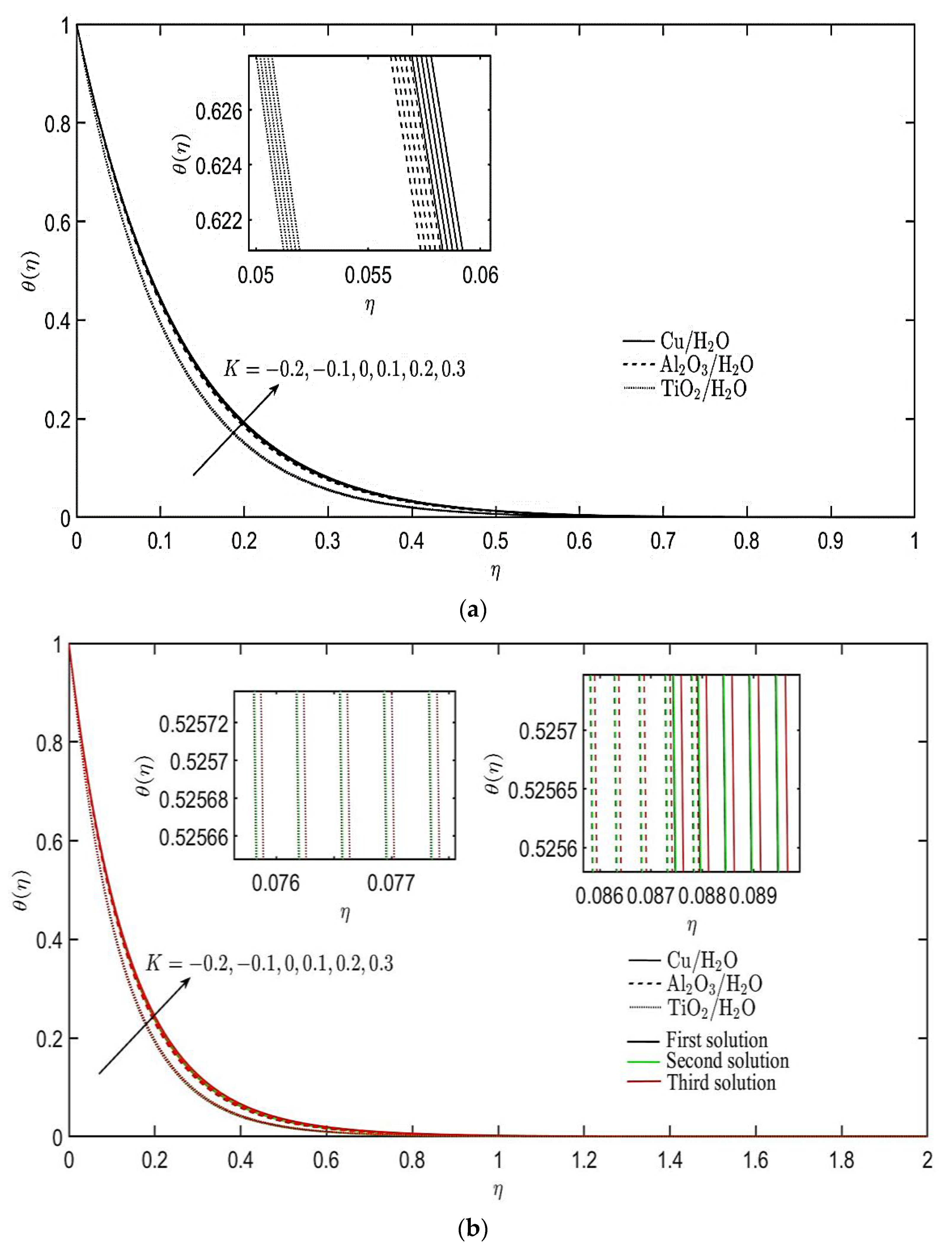
• The temperature profile is also augmented by the increment of the heat source parameter but diminished with the heat sink parameter.
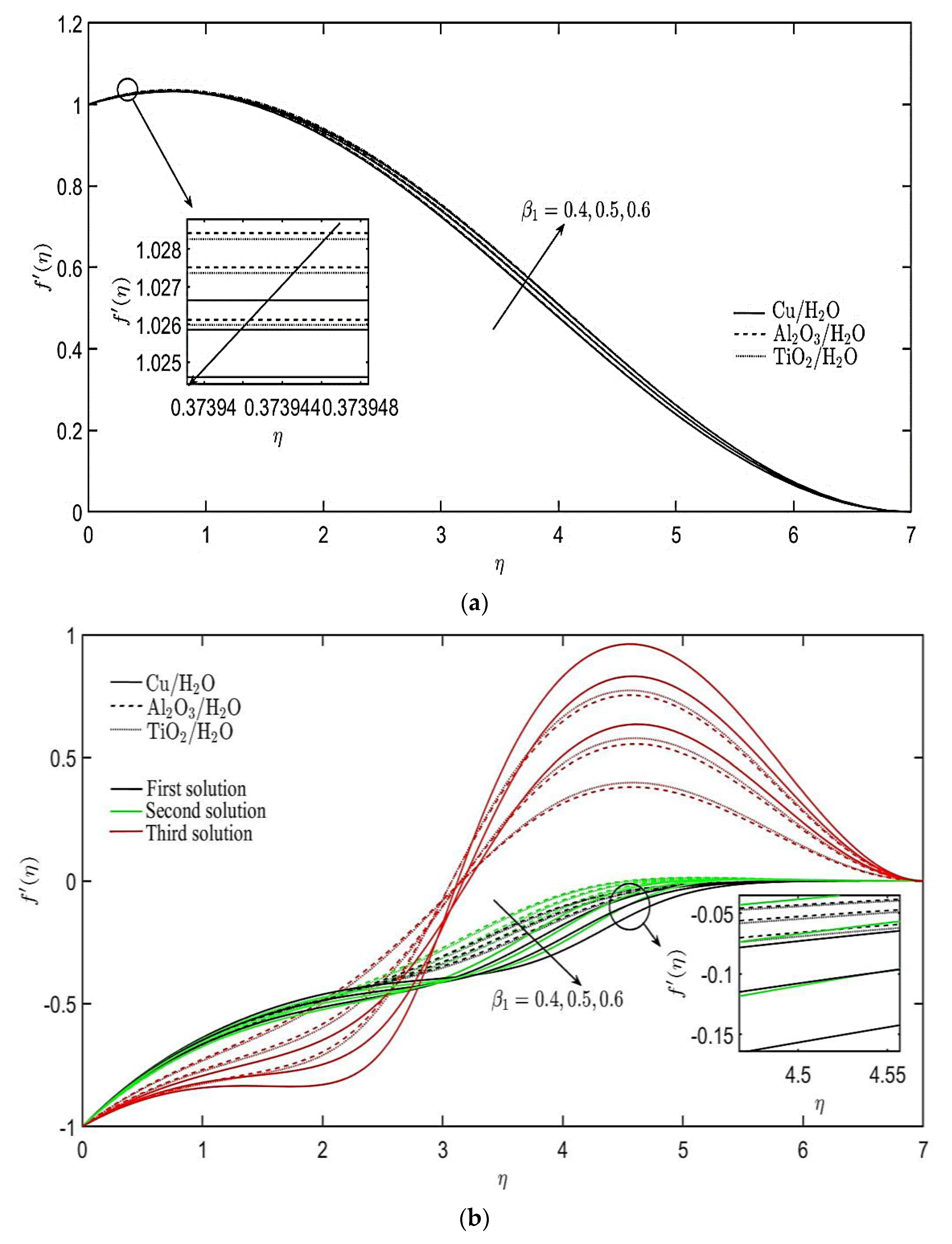
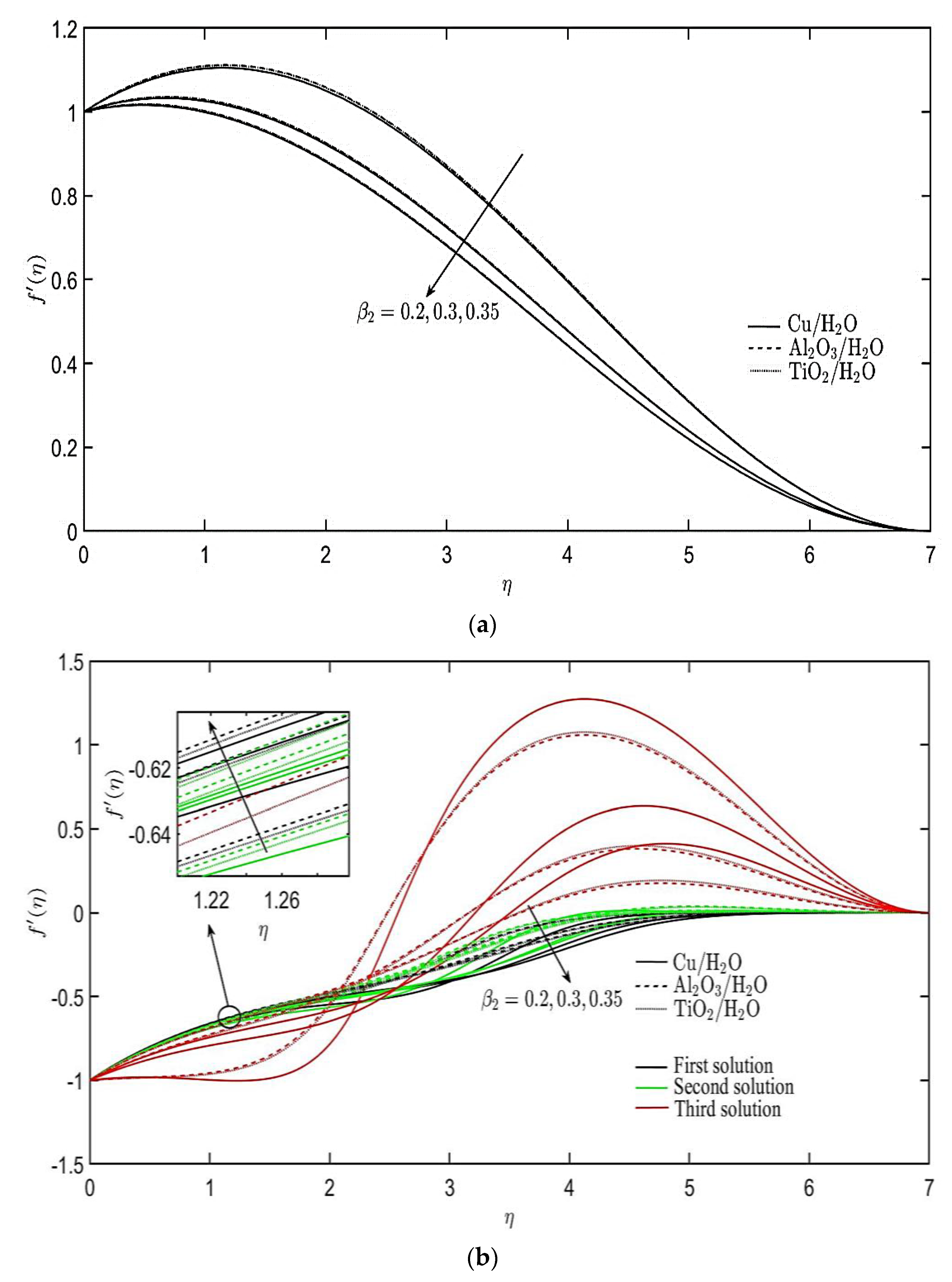
• The non-Newtonian parameters related to Burgers’ fluid have different effects on the velocity and temperature profiles of the nanofluids for both cases of stretching and shrinking sheets.

This study can be extended to different flow geometries, such as Burgers’ nanofluids flow over a stretching cylinder or between a cone and disk, and other physical conditions, such as entropy generation, variable concentration, and chemical reaction. Furthermore, this study can be expanded to suit the current application of heat transfer fluid, for example, in double pipe heat exchangers. Since this is a theoretical study, the experimental investigation of this flow problem is also encouraged.

References

1. Khan, M.; Iqbal, Z.; Ahmed, A. Energy transport analysis in the flow of burgers nanofluid inspired by variable thermal conductivity. Pramana 2021, 95, 74. [Google Scholar] [CrossRef]
2. Hayat, T.; Fetecau, C.; Asghar, S. Some simple flows of a burgers’ fluid. Int. J. Eng. Sci. 2006, 44, 1423–1431. [Google Scholar] [CrossRef]
3. Rashidi, M.M.; Yang, Z.; Awais, M.; Nawaz, M.; Hayat, T. Generalized magnetic field effects in burgers’ nanofluid model. PLoS ONE 2017, 12, e0168923. [Google Scholar] [CrossRef] [PubMed]
4. Alsaedi, A.; Alsaadi, F.E.; Ali, S.; Hayat, T. Stagnation point flow of burgers’ fluid and mass transfer with chemical reaction and porosity. J. Mech. 2012, 29, 453–460. [Google Scholar] [CrossRef]
5. Hayat, T.; Ali, S.; Awais, M.; Obaidat, S. Stagnation point flow of burgers’ fluid over a stretching surface. Prog. Comput. Fluid Dyn. Int. J. 2013, 13, 48–53. [Google Scholar] [CrossRef]
6. Hayat, T.; Ali, S.; Awais, M.; Alsaedi, A. Joule heating effects in mhd flow of burgers’ fluid. Heat Transf. Res. 2016, 47, 1083–1092. [Google Scholar] [CrossRef]
7. Hayat, T.; Asad, S.; Alaseadi, A. Mhd mixed convection flow of burgers’ fluid in a thermally stratified medium. J. Aerosp. Eng. 2016, 29, 04016060. [Google Scholar] [CrossRef]
8. Hayat, T.; Waqas, M.; Khan, M.I.; Alsaedi, A.; Shehzad, S.A. Magnetohydrodynamic flow of burgers fluid with heat source and power law heat flux. Chin. J. Phys. 2017, 55, 318–330. [Google Scholar] [CrossRef]
9. Ahmad, I.; Ali, N.; Abbasi, A.; Aziz, W.; Hussain, M.; Ahmad, M.; Taj, M.; Zaman, Q. Flow of a burger’s fluid in a channel induced by peristaltic compliant walls. J. Appl. Math. 2014, 2014, 236483. [Google Scholar] [CrossRef] [Green Version]
10. Khan, N.A.; Khan, S.; Ullah, S. Mhd flow of burger’s fluid over an off-centered rotating disk in a porous medium. AIP Adv. 2015, 5, 087179. [Google Scholar] [CrossRef] [Green Version]
11. Imran, M.; Ching, D.L.C.; Safdar, R.; Khan, I.; Imran, M.A.; Nisar, K.S. The solutions of non-integer order burgers’ fluid flowing through a round channel with semi analytical technique. Symmetry 2019, 11, 962. [Google Scholar] [CrossRef] [Green Version]
12. Safdar, R.; Imran, M.; Tahir, M.; Sadiq, N.; Imran, M.A. MHD Flow of Burgers’ Fluid under the Effect of Pressure Gradient Through a Porous Material Pipe. Punjab Univ. J. Math. 2018, 50, 73–90. [Google Scholar]
13. Akram, S.; Anjum, A.; Khan, M.; Hussain, A. On stokes’ second problem for burgers’ fluid over a plane wall. J. Appl. Comput. Mech. 2021, 7, 1514–1526. [Google Scholar] [CrossRef]
14. Jiang, Y.; Sun, H.; Bai, Y.; Zhang, Y. MHD flow, radiation heat and mass transfer of fractional Burgers’ fluid in porous medium with chemical reaction. Comput. Math. Appl. 2022, 115, 68–79. [Google Scholar] [CrossRef]
15. Gangadhar, K.; Kumari, M.A.; Rao, M.V.S.; Alnefaie, K.; Khan, I.; Andualem, M. Magnetization for burgers’ fluid subject to convective heating and heterogeneous-homogeneous reactions. Math. Probl. Eng. 2022, 2022, 2747676. [Google Scholar] [CrossRef]
16. Choi, S.U.S.; Eastman, J.A. Enhancing Thermal Conductivity of Fluids with Nanoparticles; Argonne National Lab. (ANL): Argonne, IL, USA, 1995.
17. Alghamdi, M. Significance of arrhenius activation energy and binary chemical reaction in mixed convection flow of nanofluid due to a rotating disk. Coatings 2020, 10, 86. [Google Scholar] [CrossRef] [Green Version]
18. Khan, M.I.; Alzahrani, F. Activation energy and binary chemical reaction effect in nonlinear thermal radiative stagnation point flow of walter-b nanofluid: Numerical computations. Int. J. Mod. Phys. B 2020, 34, 2050132. [Google Scholar] [CrossRef]
19. Hayat, T.; Waqas, M.; Shehzad, S.A.; Alsaedi, A. On model of burgers fluid subject to magneto nanoparticles and convective conditions. J. Mol. Liq. 2016, 222, 181–187. [Google Scholar] [CrossRef]
20. Hayat, T.; Waqas, M.; Shehzad, S.A.; Alsaedi, A. Mixed convection flow of a burgers nanofluid in the presence of stratifications and heat generation/absorption. Eur. Phys. J. Plus 2016, 131, 253. [Google Scholar] [CrossRef]
21. Iqbal, Z.; Khan, M.; Ahmed, A.; Ahmed, J.; Hafeez, A. Thermal energy transport in burgers nanofluid flow featuring the cattaneo–christov double diffusion theory. Appl. Nanosci. 2020, 10, 5331–5342. [Google Scholar] [CrossRef]
22. Xuan, Y.; Li, Q. Heat transfer enhancement of nanofluids. Int. J. Heat Fluid Flow 2000, 21, 58–64. [Google Scholar] [CrossRef]
23. Das, S.K.; Choi, S.U.S.; Patel, H.E. Heat transfer in nanofluids—A review. Heat Transf. Eng. 2006, 27, 3–19. [Google Scholar] [CrossRef]
24. Khattak, M.A.; Mukhtar, A.; Afaq, S.K. Application of nano-fluids as coolant in heat exchangers: A review. J. Adv. Res. Mater. Sci. 2020, 66, 8–18. [Google Scholar] [CrossRef]
25. Das, S.K.; Choi, S.U.; Yu, W.; Pradeep, T. Nanofluids: Science and Technology; John Wiley & Sons: Hoboken, NJ, USA, 2007. [Google Scholar]
26. Nield, D.A.; Bejan, A. Convection in Porous Media; Springer: Berlin/Heidelberg, Germany, 2006; Volume 3. [Google Scholar]
27. Minkowycz, W.J.; Sparrow, E.M.; Abraham, J.P. Nanoparticle Heat Transfer and Fluid Flow; CRC Press: Boca Raton, FL, USA, 2012; Volume 4. [Google Scholar]
28. Shenoy, A.; Sheremet, M.; Pop, I. Convective Flow and Heat Transfer from Wavy Surfaces: Viscous Fluids, Porous Media, and Nanofluids; CRC Press: Boca Raton, FL, USA, 2016. [Google Scholar]
29. Manca, O.; Jaluria, Y.; Poulikakos, D. Heat Transfer in Nanofluids. Advances in Mechanical Engineering; Sage Publications: London, UK, 2010; p. 380826. [Google Scholar]
30. Myers, T.G.; Ribera, H.; Cregan, V. Does Mathematics Contribute to the Nanofluid Debate? Int. J. Heat Mass Transf. 2017, 111, 279–288. [Google Scholar] [CrossRef] [Green Version]
31. Mahian, O.; Kolsi, L.; Amani, M.; Estellé, P.; Ahmadi, G.; Kleinstreuer, C.; Marshall, J.S.; Siavashi, M.; Taylor, R.A.; Niazmand, H.; et al. Recent advances in modeling and simulation of nanofluid flows-part i: Fundamentals and theory. Phys. Rep. 2019, 790, 1–48. [Google Scholar] [CrossRef]
32. Mahian, O.; Kolsi, L.; Amani, M.; Estellé, P.; Ahmadi, G.; Kleinstreuer, C.; Marshall, J.S.; Taylor, R.A.; Abu-Nada, E.; Rashidi, S. Recent advances in modeling and simulation of nanofluid flows—Part II: Applications. Phys. Rep. 2019, 791, 1–59. [Google Scholar] [CrossRef]
33. Mahian, O.; Kianifar, A.; Kalogirou, S.A.; Pop, I.; Wongwises, S. A review of the applications of nanofluids in solar energy. Int. J. Heat Mass Transf. 2013, 57, 582–594. [Google Scholar] [CrossRef]
34. Khan, M.; Khan, W.A. Forced convection analysis for generalized Burgers nanofluid flow over a stretching sheet. AIP Adv. 2015, 5, 107138. [Google Scholar] [CrossRef] [Green Version]
35. Khan, M.; Khan, W.A. Steady flow of Burgers’ nanofluid over a stretching surface with heat generation/absorption. J Braz. Soc. Mech. Sci. Eng. 2016, 38, 2359–2367. [Google Scholar] [CrossRef]
36. Buongiorno, J. Convective transport in nanofluids. J. Heat Transf. 2006, 128, 240–250. [Google Scholar] [CrossRef]
37. Muhammad, S.; Ishaq, M.; Hussain, S.A.; Tahir, M.; Naeem, M.; Khan, H.; Jan, S.; Khan, K. Semi analytical solution of steady Burgers’ nanofluid flow between parallel channels with heat generation/absorption under the influence of thermal radiation. J. Nanofluids 2019, 8, 1468–1478. [Google Scholar] [CrossRef]
38. Khan, M.; Iqbal, Z.; Ahmed, A. Stagnation point flow of magnetized burgers’ nanofluid subject to thermal radiation. Appl. Nanosci. 2020, 10, 5233–5246. [Google Scholar] [CrossRef]
39. Khan, S.U.; Alabdan, R.; Al-Qawasmi, A.-R.; Vakkar, A.; ben Handa, M.; Tlili, I. Bioconvection applications for double stratification 3-d flow of burgers nanofluid over a bidirectional stretched surface: Enhancing energy system performance. Case Stud. Therm. Eng. 2021, 26, 101073. [Google Scholar] [CrossRef]
40. Waqas, H.; Manzoor, U.; Shah, Z.; Arif, M.; Shutaywi, M. Magneto-burgers nanofluid stratified flow with swimming motile microorganisms and dual variables conductivity configured by a stretching cylinder/plate. Math. Probl. Eng. 2021, 2021, 8817435. [Google Scholar] [CrossRef]
41. Ramzan, M.; Algehyne, E.A.; Saeed, A.; Dawar, A.; Kumam, P.; Watthayu, W. Homotopic simulation for heat transport phenomenon of the Burgers nanofluids flow over a stretching cylinder with thermal convective and zero mass flux conditions. Nanotechnol. Rev. 2022, 11, 1437–1449. [Google Scholar] [CrossRef]
42. Wang, F.; Iqbal, Z.; Zhang, J.; Abdelmohimen, M.A.H.; Almaliki, A.H.; Galal, A.M. Bidirectional stretching features on the flow and heat transport of Burgers nanofluid subject to modified heat and mass fluxes. Waves Random Complex Media 2022, 1–18. [Google Scholar] [CrossRef]
43. Tiwari, R.K.; Das, M.K. Heat transfer augmentation in a two-sided lid-driven differentially heated square cavity utilizing nanofluids. Int. J. Heat Mass Transf. 2007, 50, 2002–2018. [Google Scholar] [CrossRef]
44. Pop, I.; Seddighi, S.; Bachok, N.; Ismail, F. Boundary layer flow beneath a uniform free stream permeable continuous moving surface in a nanofluid. J. Heat Mass Transf. Res. 2014, 1, 55–65. [Google Scholar] [CrossRef]
45. Ejaz, A.; Abbas, I.; Nawaz, Y.; Arif, M.S.; Shatanawi, W.; Abbasi, J.N. Thermal analysis of mhd non-newtonian nanofluids over a porous media. CMES—Comput. Model. Eng. Sci. 2020, 125, 1119–1134. [Google Scholar] [CrossRef]
46. Ho, C.J.; Liu, W.K.; Chang, Y.S.; Lin, C.C. Natural convection heat transfer of alumina-water nanofluid in vertical square enclosures: An experimental study. Int. J. Therm. Sci. 2010, 49, 1345–1353. [Google Scholar] [CrossRef]
47. Sheremet, M.A.; Pop, I.; Rosca, A.V. The influence of thermal radiation on unsteady free convection in inclined enclosures filled by a nanofluid with sinusoidal boundary conditions. Int. J. Numer. Methods Heat Fluid Flow 2018, 28, 1738–1753. [Google Scholar] [CrossRef]
48. Oztop, H.F.; Abu-Nada, E. Numerical study of natural convection in partially heated rectangular enclosures filled with nanofluids. Int. J. Heat Fluid Flow 2008, 29, 1326–1336. [Google Scholar] [CrossRef]
49. Fang, T.; Yao, S.; Zhang, J.; Aziz, A. Viscous flow over a shrinking sheet with a second order slip flow model. Commun. Nonlinear Sci. Numer. Simul. 2010, 15, 1831–1842. [Google Scholar] [CrossRef]
50. Vajravelu, K.; Rollins, D. Hydromagnetic flow of a second grade fluid over a stretching sheet. Appl. Math. Comput. 2004, 148, 783–791. [Google Scholar] [CrossRef]
51. Cortell, R. Viscous flow and heat transfer over a nonlinearly stretching sheet. Appl. Math. Comput. 2007, 184, 864–873. [Google Scholar] [CrossRef]
52. Crane, L.J. Flow past a stretching plate. Z. Angew. Math. Phys. ZAMP 1970, 21, 645–647. [Google Scholar] [CrossRef]
53. Weidman, P.D.; Kubitschek, D.G.; Davis, A.M.J. The effect of transpiration on self-similar boundary layer flow over moving surfaces. Int. J. Eng. Sci. 2006, 44, 730–737. [Google Scholar] [CrossRef]
54. Roşca, A.V.; Pop, I. Flow and heat transfer over a vertical permeable stretching/shrinking sheet with a second order slip. Int. J. Heat Mass Transf. 2013, 60, 355–364. [Google Scholar] [CrossRef]
55. Wahid, N.S.; Arifin, N.M.; Khashi’ie, N.S.; Pop, I. Hybrid nanofluid slip flow over an exponentially stretching/shrinking permeable sheet with heat generation. Mathematics 2020, 9, 30. [Google Scholar] [CrossRef]
56. Lund, L.A.; Omar, Z.; Khan, U.; Khan, I.; Baleanu, D.; Nisar, K.S. Stability analysis and dual solutions of micropolar nanofluid over the inclined stretching/shrinking surface with convective boundary condition. Symmetry 2020, 12, 74. [Google Scholar] [CrossRef] [Green Version]
57. Yahaya, R.I.; Md Arifin, N.; Mohamed Isa, S.S.P.; Rashidi, M.M. Magnetohydrodynamics boundary layer flow of micropolar fluid over an exponentially shrinking sheet with thermal radiation: Triple solutions and stability analysis. Math. Methods Appl. Sci. 2021, 44, 10578–10608. [Google Scholar] [CrossRef]
58. Harris, S.D.; Ingham, D.B.; Pop, I. Mixed convection boundary-layer flow near the stagnation point on a vertical surface in a porous medium: Brinkman model with slip. Transp. Porous Media 2009, 77, 267–285. [Google Scholar] [CrossRef]
59. Zainal, N.A.; Nazar, R.; Naganthran, K.; Pop, I. Stability analysis of unsteady mhd rear stagnation point flow of hybrid nanofluid. Mathematics 2021, 9, 2428. [Google Scholar] [CrossRef]
60. Khashi’ie, N.S.; Arifin, N.M.; Merkin, J.H.; Yahaya, R.I.; Pop, I. Mixed convective stagnation point flow of a hybrid nanofluid toward a vertical cylinder. Int. J. Numer. Methods Heat Fluid Flow 2021, 31, 3689–3710. [Google Scholar] [CrossRef]
61. Yahaya, R.I.; Md Arifin, N.; Nazar, R.M.; Pop, I. Oblique stagnation-point flow past a shrinking surface in a Cu-Al2O3/H2O hybrid nanofluid. Sains Malays. 2021, 50, 3139–3152. [Google Scholar] [CrossRef]
62. Pantokratoras, A. A common error made in investigation of boundary layer flows. Appl. Math. Model. 2009, 33, 413–422. [Google Scholar] [CrossRef]
63. Rahman, M.M.; Ariz, A. Heat transfer in water based nanofluids (TiO2-H2O, Al2O3-H2O and Cu-H2O) over a stretching cylinder. Int. J. Heat Technol. 2012, 30, 31–42. [Google Scholar] [CrossRef]
64. Dawar, A.; Bonyah, E.; Islam, S.; Alshehri, A.; Shah, Z. Theoretical analysis of Cu-H2O, Al2O3-H2O, and TiO2-H2O nanofluid flow past a rotating disk with velocity slip and convective conditions. J. Nanomater. 2021, 2021, 5471813. [Google Scholar] [CrossRef]
Figure 1. Physical model for: (a) Stretching sheet (λ > 0); (b) Shrinking sheet (λ < 0) [44].
Mathematics 10 01580 g001
Figure 2. Velocity profiles of different nanofluids for: (a) Stretching case; (b) Shrinking case.
Mathematics 10 01580 g002
Figure 3. Temperature profiles of different nanofluids for: (a) Stretching case; (b) Shrinking case.
Mathematics 10 01580 g003
Figure 4. Effect of nanoparticle volume fraction on velocity profiles for: (a) Stretching case; (b) Shrinking case.
Mathematics 10 01580 g004
Figure 5. Effect of nanoparticle volume fraction on temperature profiles for: (a) Stretching case; (b) Shrinking case.
Mathematics 10 01580 g005
Figure 6. Effect of heat source/sink parameter on temperature profiles for: (a) Stretching case; (b) Shrinking case.
Mathematics 10 01580 g006
Figure 7. Effect of fluid relaxation time parameter on velocity profile for: (a) Stretching case; (b) Shrinking case.
Mathematics 10 01580 g007
Figure 8. Effect of fluid relaxation time parameter on temperature profiles for: (a) Stretching case; (b) Shrinking case.
Mathematics 10 01580 g008
Figure 9. Effect of Burgers’ fluid parameter on velocity profiles for: (a) Stretching case; (b) Shrinking case.
Mathematics 10 01580 g009
Figure 10. Effect of Burgers’ fluid parameter on temperature profiles for: (a) Stretching case; (b) Shrinking case.
Mathematics 10 01580 g010
Figure 11. Effect of fluid retardation time parameter on velocity profiles for: (a) Stretching case; (b) Shrinking case.
Mathematics 10 01580 g011
Figure 12. Effect of fluid retardation time parameter on temperature profiles for: (a) Stretching case; (b) Shrinking case.
Mathematics 10 01580 g012