Article

The Impact of Options on Investment Portfolios in the Short-Run and the Long-Run, with a Focus on Downside Protection and Call Overwriting

8 Highview, Caterham CR3 6AY, UK
Mathematics 2022, 10(9), 1563; https://doi.org/10.3390/math10091563
Submission received: 4 April 2022 / Revised: 28 April 2022 / Accepted: 29 April 2022 / Published: 6 May 2022

Abstract

:
In this article, we analyse the impact of the introduction of options on an investment portfolio. Our first objective is to derive closed-form formulae for the standard measures of portfolio efficiency: risk premium, risk, Sharpe ratio, and beta, of any portfolio containing any combination of options. Using these formulae on three examples of simple option strategies (call overwriting, put protection, and collars), we show how these statistics are altered by the inclusion of an option overlay in a portfolio. Our second objective is to show that if an option strategy is repeated over multiple investment time periods, the long-run return becomes normally distributed. Our motivation is to provide investors with the mathematics to measure the impact of the introduction of options on portfolio efficiency and encourage a potential portfolio rebalance to account for this impact. Then, we highlight that whilst options can create asymmetric non-normal outcomes, their repeated use may not alter the long-run portfolio return in the desired way and thus to encourage investors to assess if an option overlay will deliver the desired long-run outcome.

1. Introduction

Options are derivative instruments that alter the characteristics of an underlying asset. They can be added to an investment portfolio to engineer desired outcomes. In some sense, they improve portfolio efficiency by providing downside protection and enhancing the income of a portfolio.
Options specialists measure risk using the so-called Greeks (e.g., delta, gamma, theta, vega) [1], which are not the conventional measures of portfolio efficiency in the asset management industry. The latter typically measure a portfolio’s future return distribution with the three summary statistics expected return, risk, and the portfolio beta (the return sensitivity of the portfolio relative to the market) [2]. Consequently, options are used in asset management with scant regard for their impact on these summary statistics.
The first objective of this paper is to derive formulae for expected return, risk, and beta for portfolios that contain options, not just for specific or simple option strategies, but general formulae to be applied to any possible option strategy.
In the first half of this article, we introduce options and define the return of a portfolio involving options, being careful to avoid ambiguity on cost and leverage. We then provide closed-form expressions for these summary statistics (expected return, risk, and beta) for a portfolio containing any option strategy. We apply these formulae in three worked examples of popular option strategies: income enhancement (call overwriting), downside protection (put protection), and reduced cost downside protection (a collar strategy). We will see that the beta of the portfolio is reduced by the inclusion of options. We will further see in these examples that both the expected return and risk are also reduced, but at differing rates so that the Sharpe Ratio of the portfolio is impacted by these option strategies. That is to say, the efficiency of portfolios may be reduced by the introduction of options. The materiality of these reductions depends significantly on the option strike prices.
Our motivation for deriving these single-period return statistics is to enable investors to assess the impact of options on investment portfolios, using the standard measures. With these measures, we encourage portfolio managers to: (i) be judicious in the choice of strike prices in light of the influence of strike price on return, risk, and beta; (ii) assess whether the investors’ return, risk, and beta targets are still met when options are deployed; and (iii) rebalance the portfolio accordingly if summary statistic targets are missed as a consequence of overlaying an option strategy.
The second objective of this article is to identify the probability distribution of portfolio long-run return when option strategies are repeated over time.
The time horizon is important when options are used in investment portfolios. An option strategy is over a single period, which is typically three months and seldom greater than a year, whereas the horizon of long-term investors is significantly longer. For example, pension funds have triennial valuations and can invest with a time horizon far longer than even that. In the second part of this article, we will consider the long-term return distribution of an investment portfolio which includes an option strategy that is sequentially repeated (a quarterly call overwriting strategy repeated 12 times in a 3 years, would be an example). We will define when an option strategy is invariant over time, then prove that any invariant option strategy that is sequentially repeated has a long-term investment portfolio return that tends to a normal distribution. Using simulations, we will demonstrate this result for our three example strategies, showing that the convergence to a normal distribution is fast but does depend on the strike price.
Our motivation for deriving this long-run return distribution is two-fold. First, as measures of portfolio efficiency, the summary statistics of expected return, risk, and beta are used to construct and assess investment portfolios. That is only theoretically valid if the portfolio return is normally distributed. The use of these summary statistics is considered appropriate on portfolios of conventional assets (such as equities and bonds) because empirical evidence suggests that returns of these assets appear close to being normally distributed, especially for holding periods of a month or more [3] (and references therein). However, given that options specifically create asymmetry, single investment period returns of portfolios containing options will be non-normal, and these statistics may not be valid in this case [4]. Showing that returns of portfolios containing option strategies tend to a normal distribution over time implies the summary statistics can be used over longer investment horizons, even if asymmetry is present in the short term. Second, we use this result to caution portfolio managers against sequentially repeating option strategies if portfolio efficiency is taken to be the asymmetry of return over the longer term.
Multi-asset portfolios are seeing an increase in popularity owing to their improved portfolio efficiency over equities [5]. Although options have traditionally been used in equity portfolios, they are now seeing widespread use in these multi-asset portfolios. For example: multi-asset income funds commonly use call overwriting strategies to boost distributable income; diversified growth funds can use options to provide protected leverage. Moreover, balanced funds, especially those used in pension management, are seeing increased use in protection strategies on the risky elements of the portfolio. Therefore, we intend our results to be applicable to both equity and multi-asset investors. As multi-asset investing continues its current expansion into solution design, the use of options is expanding, as is the sophistication of the option strategies deployed. The purpose of our general formulae is to ensure the impact of options on those portfolios can be measured, regardless of their sophistication.

2. Literature Review

There is a body of literature that endeavours to compute instantaneous risk statistics, notably [6]. This includes the measurement of instantaneous betas in [7]. However, our interest is not in the measurement of these statistics at an instantaneous point in time in the life of the option, it is to provide measures over the life of the option.
Papers providing a theoretical framework for deriving return and risk statistics over the life of the options are extant but tend to focus on specific strategies. For example, Figelman [8] provided a formulation for covered-call strategies, and Goetzmann et al. [9] provided risk and expected return formulae for portfolios consisting of up to two options.
There have been many empirical studies measuring ex-post risks and returns of option-adjusted portfolios. Israelov and Klein [10] analysed return and risk of collars. Slivka [11] measured the risk of numerous option strategies, including call overwriting and put protection. Merton, Scholes, and Gladstein [12] simulated call overwriting with various strike prices on historic stock data. The aforementioned authors repeated their study for put protection in [13]. These studies can be used to validate our formulae, and we will do that later in the article, but we share, and stress, Bollen’s view [14] that practical investment management requires forward-looking ex-ante measures that account for the entire distribution of possible future payoffs. Bollen’s view is the motivation for the objectives of this article.
The published work conceptually closest to this article is the collection of articles by Bookstaber and Clarke relating to the distribution of returns of option-adjusted portfolios as laid out in [15]. In [16], they provided an algorithm for computing the return distribution of an option-adjusted portfolio and applied their algorithm to simple call and put strategies in [4]. Bookstaber and Clark [17] were able to form histograms of the returns from these strategies, but they conceded that it was not possible to derive the probability distributions. Although the full distribution cannot be derived, the contribution of this paper is to provide closed-form formulae for the summary statistics: expected return, risk, and beta. We emphasise that we have extended the existing literature, not just because we have provided closed-form formulae for these statistics, but because our formulae are general and can be applied to any option strategy.

3. Options

3.1. Definitions Relating to Options

A call option on an underlying security is the right but not the obligation to buy that security at a preset price on a specified future date. The preset price is termed the strike price, and the specified future date is termed the expiry date. The value of the call option on the expiry date is max ( x k , 0 ) , where k denotes the strike price and x denotes the value of the underlying security on the expiry date of the option (we will use the denotation of x for the remainder of this article). Note that since the value of the call option at expiry is never negative, but sometimes positive, the call option must have a non-zero cost to purchase.
Whereas a call option is the right to buy an underlying security, a put option is the right to sell that security.
An option is visually represented by a graph of the value of the option at expiry as a function of the underlying asset price (termed a payoff profile [18]). The payoff profiles for a call and put option are shown in Figure 1.
The difference between the strike price and the underlying asset price as a proportion of the underlying asset price is termed the option’s moneyness. If the strike price is less than the asset price, a call option is said to be in-the-money; if the strike price is more than the asset price, a call option is out-of-the-money (for put options the reverse is true). For example, a call option with a strike of 95 on an underlying asset with a price of 100 is 5% in-the-money. Options with a strike price equal to the asset price are termed at-the-money.

3.2. Examples of Option Strategies

To demonstrate the concepts in this article, we will apply them to three examples of commonly used option strategies:
1.
Call overwriting is the selling of a call option on an underlying asset that is already owned. The investor receives the price of a call option in lieu of a sacrifice of underlying asset price appreciation beyond a specified price. Call overwriting is commonly used to boost income from the underlying security which is usually either an individual equity security or an equity index [19].
2.
Put protection is the buying of a put option on an underlying asset that is already owned. The option price is paid by the investor in exchange for a guaranteed minimum underlying asset price on the expiry date, akin to an insurance payment. Put protection is often applied to equity indices, where the guarantee is set to be the purchase price of the index, thereby providing capital protection [19].
3.
Collar is a combination of put protection and call overwriting, whereby protection is sought but upside is sacrificed to offset the cost of protection [20].
The payoff profiles of these three strategies are shown in Figure 2. The first panel shows the payoff profile of call overwriting overlaid on a portfolio containing the underlying asset. We can see that this payoff profile is identical to selling a put option. The second panel shows the payoff profile of put protection overlaid on a portfolio containing the underlying asset. We can see that this payoff profile is identical to buying a call option. The third panel shows the payoff profile of a collar, where both underlying asset price appreciation and depreciation are capped. This strategy can be overlaid on an underlying asset by buying a put and selling a call. If the underlying asset is not owned, a collar is constructed by buying a call and selling a put.
If preferred, the underlying asset can be considered separately, with an option strategy overlaid, or the underlying asset can be considered as part of the option strategy. Mathematically, these are equivalent, and in this article, we will express strategies in either way to facilitate readability.

3.3. Portfolios including Options

This article addresses the impact of using options to engineer the payoff profile of a portfolio. We will hereafter, except for Section 4.4, assume there is one risky asset. This could be a single security or an entire market portfolio. To simplify the mathematics of this article, we will assume non-dividend-paying underlying assets. It is a routine algebraic exercise for the reader to incorporate dividends into the formulae shown here.
We will also assume that a risk-free asset exists. Therefore, in our context, a traditional portfolio comprises solely the risk-free asset and the risky asset. To distinguish portfolios containing options, we define an option-adjusted portfolio to refer specifically to a traditional portfolio which also contains options on the risky asset. The option-adjusted portfolio can contain multiple options with potentially differing strike prices, but for mathematical convenience, we will restrict them to all having the same expiry date. We show in Appendix that the payoff profile of any option-adjusted portfolio is a continuous piecewise linear function of the underlying security price at the time of expiry. Letting x 1 , …, x n denote the strike prices of n options (ordered such that x 1 < x 2 < < x n ) and using x 0 and x n + 1 to denote the upper and lower limits of the underlying asset price, hence x 0 = 0 and x n + 1 = , we can write the option-adjusted portfolio value at expiry, denoted by v ( x ) , as
v ( x ) = a i + b i ( x x i ) for   x i x < x i + 1
where a 0 , …, a n are the intercepts, and b 0 , …, b n are the gradients of each segment. Specifically, a 0 represents the value at expiry of the cash holding; b 0 represents the number of the risky asset units held in the portfolio; and b 1 , …, b n are governed by the quantities of the options where b i equals b i 1 plus the number of units of the ith call option held in the portfolio. The intercepts a 1 , …, a n are calculated using the formula a i = a i 1 + b i 1 ( x i x i 1 ) . This piecewise linear representation has a useful application as it is often easier to sketch the desired payoff profile of a portfolio, then calculate what options need to be purchased to create that. For example, we see in Appendix A that to replicate a payoff profile made up of linear segments joined at x 1 , …, x n , with intercepts a 0 , …, a n , and gradients b 0 , …, b n , the investor can hold ( a 0 ÷ risk-free asset end value) units of the risk-free asset; hold b 0 units of the risky asset; and hold ( b i b i 1 ) units of a call option with strike price x i (for i = 1, …, n). We also see in Appendix A that our summary statistics are unaffected by a vertical shift of the payoff profile; therefore, we can assume without loss of generality that a 0 = 0 .
The input parameters for our three example strategies are shown in Table 1.

3.4. Investment Returns of Option-Adjusted Portfolios

The return on an investment is the change in its price as a proportion of the initial investment value. Trivially, the return on the underlying asset, denoted by r A , is
r A = x s 1
where s denotes the initial underlying security value.
The return on the option-adjusted portfolio needs a more careful definition. In practice, portfolio wealth is largely invested in the underlying asset, and the option strategy is overlaid on that. However, it is mathematically irrelevant whether we consider the portfolio as containing an investment in the underlying asset and an option strategy overlaid on that or an investment in the risk-free asset and an option strategy overlaid on that, where the investment in the underlying asset is subsumed in the option strategy (this is an extension of put-call parity where the payoff of a call and cash is the same of a put and the underlying asset [1] (p. 163)). For algebraic brevity, we will assume the latter. This enables us to consider the portfolio as if it consisted of an investment in the risk-free asset, an option strategy, and a loan taken out to purchase the option strategy. In practice, portfolios often contain some cash which could be used to purchase options, or if the portfolio is fully invested in the risky asset, the options could be purchased by borrowing capital. We will assume the same rate of interest exists for both lending and borrowing to remove the complexity regarding the source of funds for option purchases.
Therefore, the return on the option-adjusted portfolio with payoff profile v ( x ) , denoted by r O , is expressed as:
r O = v ( x ) s p s ( 1 + r F ) + r F
where p denotes the cost of the option portfolio, and r F denotes the risk-free rate of return until the expiry date.
The choice of denominator in the return calculation of an option-adjusted portfolio is somewhat arbitrary because the payoff profile can be scaled by any amount by scaling each b i . However, the unit of scale of each b i is the quantity of units held in the underlying asset. Therefore, we divide by the unit price of the underlying asset when calculating portfolio return. Defining the option strategy return in this way ensures consistency. If the option strategy payoff profile is simply the value of the underlying asset, i.e., v ( x ) = x , then p = s , in which case r O = r A .

4. Summary Statistics

At the start of the investment period, s is known, but x is unknown; therefore r A is a random variable. The purpose of this article is to relate the summary statistics of the option strategies to those of the underlying asset. We will therefore assume that the expected return and the variance of the return of the underlying asset which we will denote by E [ r A ] and V [ r A ] are known.
Similarly, r O is also a random variable. In the remainder of this section, we will derive expressions for the summary statistics of r O . Specifically, we will be considering three commonly used statistics [2]:
1.
Annualised option-adjusted portfolio risk premium. Defined as ( E [ r O ] r F ) / t ;
2.
Annualised option-adjusted portfolio risk. Defined as V [ r O ] / t ;
3.
Beta of the option-adjusted portfolio with respect to the underlying asset. Defined as COV [ r O , r A ] / V [ r A ] where E [ . ] , V [ . ] , and COV [ . ] denote the expectation, variance, and covariance operators, respectively.
These statistics are annualised; hence, they are divided by t, the time remaining until the option expiry date.

4.1. Implied Volatility

The expected return of an option depends on the volatility of the underlying asset return. Therefore, the price of an option is also a function of this volatility. If we know the price of an option, we can deduce the level of volatility that must be implied by this price, termed the implied volatility. When computing the implied volatility of a series of call options with differing strike prices, we typically observe that the implied volatility is higher for lower strike prices, termed the volatility skew.
At the time of writing, 3 December 2021, the implied volatilities on options on the S&P 500 expiring on 31 March 2022, using the closing prices quoted by CBOE, exhibited this characteristic as can be seen in Figure 3.
This volatility skew accounts for uncertainty in the pricing models and reflects the risk averse nature of investors. Since both diminish in impact as the strike price of a call option increases, the implied volatility premium decreases as strike price increases, thus causing the skew.
A call option with a very high strike price is extremely unlikely to be exercised; thus the model risk in pricing such an option is minimal. Therefore, the implied volatility of deep out-of-the-money options could be considered as the market’s estimate of the volatility of the asset. In this case, there is always an increasingly large premium to be paid by the purchaser of a call option (or received by the seller of it) as the strike price decreases.
In the worked examples, we will show how material this volatility skew is on the risk premium of an option-adjusted portfolio. After suggesting a typical value for actual volatility, we will estimate the corresponding implied volatilities by adding an implied volatility premium equal to the difference between the implied volatility as of 3 December 2021 and the minimum implied volatility across all strike prices on that day.
Implied volatility does not affect the risk and beta statistics but does affect the risk premium. It is conceptually obvious that the cost of a call option will equal the underlying asset price when its strike price is zero and decrease to zero as the strike price increases. However, the volatility skew causes the price to decrease more slowly when the strike price is less than the asset price, thereby rendering those options more expensive than if the volatility skew was not present. To illustrate the impact of the skew on risk premium and Sharpe ratio (defined as the ratio of the risk premium to risk), we will plot these statistics including and excluding the implied volatility premium.

4.2. The Summary Statistics of Option-Adjusted Portfolios

The first key result in this article is that the three statistics related to option-adjusted portfolio returns can be written in closed form as
r i s k   p r e m i u m = A + B ( A * + B * ) t
r i s k = C + D + 2 E ( A + B ) 2 t
b e t a = F + G Y ( A + B ) Z Y 2
where
Y = exp { μ t } a n d Z = exp { ( 2 μ + σ 2 ) t } ,
and where
A = i = 0 n A i , B = i = 0 n B i , , G = i = 0 n G i
with
A i = y i K i B i = b i ( J i q i K i ) C i = y i 2 K i D i = b i 2 ( L i 2 q i J i + q i 2 K i ) E i = y i b i ( J i q i K i ) F i = y i J i G i = b i ( L i q i J i )
where y i = a i s and q i = x i s . Moreover,
K i = Φ ( u i + 1 ) Φ ( u i ) J i = Y ( Φ ( v i + 1 ) Φ ( v i ) ) L i = Z ( Φ ( w i + 1 ) Φ ( w i ) )
where
u i = log ( q i ) ( μ 1 / 2 σ 2 ) t σ t v i = log ( q i ) ( μ + 1 / 2 σ 2 ) t σ t w i = log ( q i ) ( μ + 3 / 2 σ 2 ) t σ t
with
μ = 1 t log ( 1 + E [ r A ] ) a n d σ 2 = 1 t log 1 + V [ r A ] ( 1 + E [ r A ] ) 2
Φ ( . ) denotes the standard normal cumulative distribution function, i.e.,
Φ ( z ) = z 1 2 π exp { 1 / 2 x 2 } d x .
A * and B * are to be computed similarly to A and B, but with μ replaced with r f , defined as
r f = 1 t log ( 1 + r F )
and with σ replaced with the market’s implied volatility of the options.
We will derive these statistics in Appendix A.

4.3. Comments on These General Formulae

We have assumed the Black Scholes method to price the options [1] (p. 207). If readers want to use their own option price, then it can be substituted in place of the expression A * + B * which represents the future value of the option price at expiry expressed as a proportion of the underlying asset price.
The option price only affects the risk premium. It does not enter the calculation of risk or beta. Both of those measures are independent of option cost and are therefore robust with respect to the pricing model used to price options.
When i = 0 , u i , v i , and w i are infinitely negative and when i = n + 1 , they are infinitely positive. This causes no computational problems because these three variables only appear in the form Φ ( u i ) , Φ ( v i ) , and Φ ( w i ) , and the function Φ ( . ) is well-behaved at ± where Φ ( ) = 0 and Φ ( ) = 1 .
Both risk and beta are independent of the risk-free rate. Apart from the option price element of the risk premium expression, the risk-free rate is not used in the risk premium either. If the future values of the strike prices are initially specified, then discounted at the risk-free rate to identify x 1 , , x n , then even the risk premium is independent of the risk-free rate.
It is not strictly necessary to assume a geometric Brownian motion. Only variables J, K, L, Y, and Z depend on the distribution of asset prices. Any pricing process such as diffusion or jump diffusion processes can be adopted to compute them (although the cost of the option embedded in the risk premium expression should be checked for its validity if something other than Brownian motion is used).

4.4. A Universe Containing Multiple Risky Assets

In practice, the investment universe will usually consist of multiple risky assets. Option strategies can be applied on an asset-by-asset basis rather than on the entire portfolio. This is especially the case for call overwriting. Analogous to our portfolio nomenclature above, we term an individual asset that has an option overlay an option-adjusted asset.

4.4.1. Risk Premium

In the case of option strategies being applied to single assets, the portfolio risk premium is given by
P o r t f o l i o   r i s k   p r e m i u m = i = 1 N w ( i ) r i s k _ p r e m i u m ( i )
where w ( i ) denotes the weight allocated to the ith asset (possibly option adjusted) and r i s k _ p r e m i u m ( i ) denotes the risk premium of the ith asset. N denotes the number of assets in the investment universe. The individual risk premium statistics can be computed as specified in the general expression in Section 4.2.

4.4.2. Risk

Portfolio risk is defined as
P o r t f o l i o   r i s k = i = 1 N w ( i ) 2 r i s k ( i ) 2 + 2 i = 1 N 1 j = i + 1 N w ( i ) w ( j ) c o v ( i j )
where r i s k ( i ) denotes the risk of the ith asset, and c o v ( i j ) denotes the covariance of the returns of asset i and asset j. The individual risk statistics, r i s k ( 1 ) , , r i s k ( N ) , can be computed as specified in the general expression in Section 4.2. However, return covariances between each pair of assets, c o v ( i j ) , are required to compute portfolio risk. The calculation of these covariances depends on whether one or both assets are option adjusted. We cover both cases below.
For notational ease, we will label the two assets Asset 1 and Asset 2. Every variable related to Asset 1 will be identified by a superscript (1) and similarly by (2) for Asset 2.
Following on from the single asset case, we will assume that the two asset prices follow geometric Brownian motion with instantaneous means μ ( 1 ) and μ ( 2 ) and instantaneous volatilities σ ( 1 ) and σ ( 2 ) but also with instantaneous correlation ρ . The value for ρ can derived from the covariance of the returns of the two underlying assets denoted by COV [ r A ( 1 ) , r A ( 2 ) ] that we will assume is known using the expression
ρ = log ( 1 + COV [ r A ( 1 ) , r A ( 2 ) ] ) σ ( 1 ) σ ( 2 ) t
Case (i)
If Asset 1 is option adjusted, but Asset 2 is not, the annualised covariance of their returns is
c o v ( i j ) = D + E ( A + B ) Y ( 2 ) t
where A and B are specified in the general expression in Section 4.2. However, D and E are now defined as follows:
D = i = 0 n D i and E = i = 0 n E i
with D i = b i ( 1 ) ( L i q i ( 1 ) J i ) and E i = y i ( 1 ) J i for i = 0 , , n .
J i = Y ( 2 ) ( Φ ( ν i + 1 ) Φ ( ν i ) ) and L i = Y ( 12 ) ( Φ ( ξ i + 1 ) Φ ( ξ i ) )
where
ν i = log ( q i ( 1 ) ) ( μ 1 / 2 ( σ ( 1 ) 2 2 ρ σ ( 1 ) σ ( 2 ) ) ) t σ ( 1 ) t ξ i = log ( q i ( 1 ) ) ( μ + 1 / 2 ( σ ( 1 ) 2 + 2 ρ σ ( 1 ) σ ( 2 ) ) ) t σ ( 1 ) t
where Y ( 1 ) = exp { μ ( 1 ) t } , Y ( 2 ) = exp { μ ( 2 ) t } , and Y ( 12 ) = Y ( 1 ) Y ( 2 ) exp { ρ σ ( 1 ) σ ( 2 ) t } .
Case (ii)
If both assets have been option adjusted, the covariance can still be computed, but the calculation is more complex. In Appendix A, we show that the covariance of returns of two option-adjusted assets is
c o v ( i j ) = C + D + E 1 + E 2 ( A ( 1 ) + B ( 1 ) ) ( A ( 2 ) + B ( 2 ) ) t
The variables A ( 1 ) , A ( 2 ) , B ( 1 ) , and B ( 2 ) are as specified in the general expression in Section 4.2 for Asset 1 and Asset 2. However, C and D, are now defined as
C = i = 0 n ( 1 ) j = 0 n ( 2 ) C i j and D = i = 0 n ( 1 ) j = 0 n ( 2 ) D i j
with C i j = y i ( 1 ) y j ( 2 ) K i j and D i j = b i ( 1 ) b j ( 2 ) ( L i i q j ( 2 ) J i j ( 1 ) q i ( 1 ) J i j ( 2 ) + q i ( 1 ) q j ( 2 ) K i j ) .
Moreover
E 1 = i = 0 n ( 1 ) j = 0 n ( 2 ) E 1 i j and E 2 = i = 0 n ( 1 ) j = 0 n ( 2 ) E 2 i j
with E 1 i j = y i ( 1 ) b j ( 2 ) ( J i j ( 2 ) q j ( 2 ) K i j ) and E 2 i j = y j ( 2 ) b i ( 1 ) ( J i j ( 1 ) q i ( 1 ) K i j ) .
The assumption of geometric Brownian motion gives us that
K i j = Φ ρ ( u i + 1 ( 1 ) , u j + 1 ( 2 ) ) Φ ρ ( u i + 1 ( 1 ) , u j ( 2 ) ) Φ ρ ( u i ( 1 ) , u j + 1 ( 2 ) ) + Φ ρ ( u i ( 1 ) , u j ( 2 ) ) J i j ( 1 ) = Y ( 1 ) Φ ρ ( v i + 1 ( 1 ) , ν j + 1 ( 2 ) ) Φ ρ ( v i + 1 ( 1 ) , ν j ( 2 ) ) Φ ρ ( v i ( 1 ) , ν j + 1 ( 2 ) ) + Φ ρ ( v i ( 1 ) , ν j ( 2 ) ) J i j ( 2 ) = Y ( 2 ) Φ ρ ( ν i + 1 ( 1 ) , v j + 1 ( 2 ) ) Φ ρ ( ν i + 1 ( 1 ) , v j ( 2 ) ) Φ ρ ( ν i ( 1 ) , v j + 1 ( 2 ) ) + Φ ρ ( ν i ( 1 ) , v j ( 2 ) ) L i j = Y ( 12 ) Φ ρ ( ξ i + 1 ( 1 ) , ξ j + 1 ( 2 ) ) Φ ρ ( ξ i + 1 ( 1 ) , ξ j ( 2 ) ) Φ ρ ( ξ i ( 1 ) , ξ j + 1 ( 2 ) ) + Φ ρ ( ξ i ( 1 ) , ξ j ( 2 ) )
where Φ ρ ( x , y ) is the cumulative distribution function of the bivariate standard normal distribution with correlation ρ .
There are numerous approached to computing Φ ρ ( x , y ) . For example, it can be expressed as
Φ ρ ( x , y ) = x 1 2 π exp { 1 / 2 z 2 } Φ y ρ z 1 ρ 2 d z
which can be solved by a one-dimensional quadrature routine.

4.4.3. Beta

In the single risky asset paradigm, we derived the beta of the option-adjusted portfolio relative to the risky asset. When there are multiple risky assets, beta is more usually measured relative to some other reference asset–-commonly a market index. Following our previous notational convention, we will denote the first and second moment of this reference asset by Y ( m ) and Z ( m ) , respectively, thus
Y ( m ) = exp { μ ( m ) t } and Z ( m ) = exp { ( 2 μ ( m ) + σ ( m ) 2 ) t } ,
In Appendix A, we show that the beta of an option-adjusted asset relative to a reference asset is
b e t a = D + E ( A + B ) Y ( m ) Z ( m ) Y ( m ) 2
where D = i = 0 n D i and E = i = 0 n E i with D i = b i ( L i q i J i ) and E i = y i J i for i = 0 , , n .
If the asset price and the reference asset price have instantaneous correlation ρ ( m ) , then
J i = Y ( m ) ( Φ ( ν i + 1 ) Φ ( ν i ) ) and L i = Y ( 1 m ) ( Φ ( ξ i + 1 ) Φ ( ξ i ) )
where
ν i = log ( q i ) ( μ 1 / 2 ( σ 2 2 ρ σ σ ( m ) ) ) t σ t ξ i = log ( q i ) ( μ + 1 / 2 ( σ 2 + 2 ρ σ σ ( m ) ) ) t σ t
where Y ( 1 m ) = Y Y ( m ) exp { ρ ( m ) σ σ ( m ) t } .
Note that ρ ( m ) can be derived from the covariance of the asset and the reference asset as follows
ρ ( m ) = log ( 1 + COV [ r A , r M ] ) σ σ ( m ) t
Once the individual asset betas have been computed, the portfolio beta is given as
P o r t f o l i o   b e t a = i = 1 N w ( i ) b e t a ( i )
where b e t a ( i ) denotes the beta of the ith asset with respect to the reference asset.

5. Examples: Single Investment Period

Let us now look at these formulae applied to our three examples.

5.1. Capital Market Assumptions

We will assume the underlying asset is an equity index (or a multi-asset diversified growth portfolio) and have therefore taken the annualised asset return E [ r A ] / t = 8 % and annualised asset risk V [ r A ] / t = 15 % . We will consider quarterly strategies and hence will set t = 0.25 . As stated earlier, the risk-free rate does not have a significant influence on the summary statistics. We set it as r F / t = 3.5 % which results in an annualised asset risk premium of 4.5 % . (Our risk premium and risk estimates are close to the capital market assumptions published by the large asset managers such as [21,22,23]). We will use the capital market assumptions stated here in all our examples hereafter.
To incorporate the implied volatility, we have subtracted the implied vol curve as of 3 December 2021 (from CBOE) from its minimum to derive an implied volatility premium, then added that to σ to generate an implied volatility curve for use in the examples below.

5.2. Call Overwriting

A call overwritten portfolio has only one strike, with a 1 equal to the strike price, and b 0 equal to 1. All other variables have zero value. Therefore, the summary statistic expressions simplify significantly. They are
r i s k   p r e m i u m = A + B ( A * + B * ) t
r i s k = C + D ( A + B ) 2 t
b e t a = F + D Y ( A + B ) Z Y 2
where A = q Φ ( u ) , B = Y Φ ( v ) , C = q 2 Φ ( u ) , D = Z Φ ( w ) , and F = q Y Φ ( v ) .
Note that for brevity we have dropped the subscripts from variables u, v, w, and q; they all refer to i = 1 in the general formulae. As stated in the general risk premium formula, A * and B * are computed similarly to A and B but with μ replaced with r f and σ replaced with the implied volatility of the option.
Call overwriting can be considered as the purchase of the underlying asset and the sale of a call option. Therefore, the implied volatility premium is in the investor’s favour. Excluding that premium, the risk premium from call overwriting strategies is zero when the strike price is very low because the payoff is highly likely to be a fixed constant value. As the strike price increases, the upside sacrifice occurs at a higher price, and therefore the call overwritten portfolio behaves more like the underlying asset. With a very high strike price, the call option is virtually indifferent from the underlying asset and therefore has the same risk premium. This can be seen Figure 4.
However, the volatility skew results in a higher premium being harvestable for lower strike prices. The increase in risk premium due to the implied volatility premium is dependent on the shape of the implied volatility curve, but using the data as of 3 December 2021, the increase in risk premium can be seen in Figure 4 to be significant for most strike prices. Indeed, for strike prices lower than the initial asset price, i.e., in-the-money options, where a guaranteed loss is made on the investment but the investor is given a premium in exchange for that loss, the risk premium increase is huge. For example, the risk premium of a call overwritten strategy with an option struck 5% in-the-money would be less than 1% excluding the boost from the implied volatility premium but is more than 7% including it.
Since the payoff is more likely to be a fixed constant as the strike price reduces, the risk of a call overwriting strategy reduces. This can be seen in Figure 5 where the risk of the portfolio is less than half of the underlying asset risk for an at-the-money option. This risk reduction makes intuitive sense because in a call overwriting strategy the price appreciation is capped, and thus there is no investment risk beyond that cap.
An important element of this paper is identifying the impact of option strategies on the portfolio Sharpe ratio. Whilst we have shown that, excluding the volatility premium, the risk premium and the portfolio risk both drop as strike price increases, they do not do so at the same rate. In fact, the risk premium drops faster. Therefore, the Sharpe ratio, being the ratio of risk premium to risk, also drops.
Figure 6 shows that this deterioration in the Sharpe ratio is modest for out-of-the-money calls (i.e., with high strike prices) and is more than offset by the boost to risk premium from the implied volatility premium. Figure 6 shows a significant increase of the Sharpe ratio when the implied volatility premium is included. For an at-the-money option, the Sharpe ratio is approximately one and continues to rise sharply as the option is struck further in-the-money.
An option can be thought of as behaving like the underlying asset when its price is sufficiently high and behaving like the risk-free asset when it is not. Consequently, the beta of the call overwriting strategy drops as the strike price drops. This is shown in Figure 7 where the reduction in beta can be seen to be large for out-of-the-money options. For example, the beta of a quarter-year call overwriting strategy when the option is struck 5% out-of-the-money has already dropped to nearly 0.6. For at-the-money options, the beta is only 0.3. Therefore, for investment strategies that target beta, a greater investment into the risky asset will be needed if a call overwriting strategy is to be overlaid.
Call overwriting is often used as an income enhancement tool by mutual funds [19], whereby the premium received for selling the call option is distributed like a dividend. Some of the growth potential of the underlying asset is sacrificed in exchange for a payment. In effect, call overwriting converts some of the capital appreciation into income. If the premium for call overwriting is distributed as income, the expected capital appreciation of the remaining portfolio is
E x p e c t e d   c a p i t a l   a p p r e c i a t i o n = A + B 1
Notice that the level of implied volatility does not affect the expected capital appreciation. The implied volatility only governs how much income is generated for a given strike price.
It is clear from this expression that the expected capital appreciation of a call overwritten portfolio can be negative. Call overwriting can turn the investment into a drawdown strategy. This may be a concern because such a portfolio will inevitably become worthless over time. To see why this is so, consider a call overwriting strategy where the call option is struck at-the-money. Then any asset price growth is sacrificed, but all asset price contraction is experienced. It is then inevitable that the expected capital appreciation is negative. The less the asset growth is sacrificed, the higher the capital appreciation of the portfolio will be. This can be seen in Figure 8 where the expected annualised capital appreciation of a quarterly call overwriting program is plotted.
The point at which the expected capital appreciation is zero can be identified by finding the strike price for which A + B = 1. This break-even strike price must clearly be greater than the initial asset price. In fact, when expected annualised asset return is 8% and its risk is 15%, this break-even strike price is 4.32% greater than the initial asset price for quarter-year options. Any call overwriting program with a strike price lower than this will cause the portfolio to become worthless if the received price of selling the call option is distributed as income. This should be born in mind especially when harvesting large option prices by selling in-the-money options. Figure 9 shows how, for a simulated price time series of the underlying asset (using the capital market assumptions stated in Section 5.1), the capital of three call overwriting strategies behaves over time using quarterly options, struck 5% in-the-money, at-the-money, and 5% out-of-the-money. The 5% in-the-money overwriting has lost 75% of its initial value in 6 years.

5.3. Put Protection

A put protected portfolio has only one strike. The payoff profile intercepts are both zero values, and only b 1 is non-zero. Therefore, our general formulae simplify significantly. We can write that for a put protected portfolio
r i s k   p r e m i u m = B B * t
r i s k = D B 2 t
b e t a = G Y B Z Y 2
where Y and Z are defined as in the general formulae, and
B = Y Φ ( v ) q Φ ( u ) D = Z Φ ( w ) 2 Y q Φ ( v ) + q 2 Φ ( u ) G = Z Φ ( w ) Y Φ ( v )
Note that for brevity we have dropped the subscripts from variables u, v, w, and q; they all refer to i = 1 in the general formulae. As stated in the general risk premium formula, B * is computed similarly to B but with μ replaced with r f and σ replaced with the implied volatility of the option.
The higher the strike price in a put protected portfolio, the more guaranteed the portfolio value is, and therefore the less risky it is. At an extreme, with infinitely high levels of protection, the portfolio is risk-free and therefore we would expect the risk premium of that portfolio to equal zero. Conversely, with no protection, the portfolio will behave identically to the underlying asset and should have the same expected return, excluding the impact of the implied volatility premium. This behaviour is indeed present when applying our formula for risk premium as can be seen in Figure 10. For example, at-the-money protection has a risk premium less than 60% of the risk premium of the underlying asset. However, the implied volatility premium has a significant effect on put protection strategies. Using the CBOE implied volatility data on options with expiry at 31 March 2022 as of 3 December 2021, Figure 10 illustrates that when protection is desired against a loss of between 0% and 10%, the implied volatility is so high that the cost of protection causes the portfolio risk premium to be negative.
In summary, the introduction of put protection lowers the expected return of a portfolio. The more protection, the more the expected return is lowered. However, the existence of an implied volatility skew can severely negatively impact this expected return.
It is intuitively obvious that the risk of the investment should drop as the guarantee increases. This effect is borne out mathematically, and the risk reduction of our protection strategy as the strike price increases as computed from our formula is presented in Figure 11.
Excluding the implied volatility premium, as the moneyness decreases, the risk premium of the put protection strategy decreases faster than the risk; therefore, the Sharpe ratio also drops. For an at-the-money strategy, the drop is from 0.3 for the underlying asset to 0.25 for the protected strategy. However, the impact of the implied volatility skew is so severe on the risk premium that once included in the computation of the Sharpe ratio, that ratio drops to −0.23. This is shown in Figure 12.
If the put protection only occurs at a low strike price, then the put protected portfolio will behave similarly to the underlying asset, and its beta will be close to one. However, as the strike price rises, the protection begins to dominate, and the beta decreases, eventually becoming zero. This behaviour can be seen in Figure 13. For protection less than 5% below market, the beta of the put protected portfolio can be seen to be above 0.8. However, beta decreases rapidly thereafter, being about 0.6 for at-the-money protection, and less than 0.4 for 5% in-the-money protection.

5.4. Collars

A collar can be overlaid on an underlying asset by buying one put and selling one call. Again, our general formulae simplify significantly for such a strategy. We can write that for a portfolio with a collar
r i s k   p r e m i u m = A + B A * B * t
r i s k = C + D ( A + B ) 2 t
b e t a = F + G Y ( A + B ) Z Y 2
where Y and Z are defined as in the general formulae, and
A = ( q c q p ) Φ ( u c ) B = Y [ Φ ( v c ) Φ ( v p ) ] q p [ Φ ( u c ) Φ ( u p ) ] C = ( q c q p ) 2 Φ ( u c ) D = Z [ Φ ( w c ) Φ ( w p ) ] 2 q p Y [ Φ ( v c ) Φ ( v p ) ] + q p 2 [ Φ ( u c ) Φ ( u p ) ] F = ( q c q p ) Y Φ ( v c ) G = Z [ Φ ( w c ) Φ ( w p ) ] q p Y [ Φ ( v c ) Φ ( v p ) ]
The subscripts p and c of variables u, v, w, and q refer to the put and the call, respectively, and map to i = 1 and i = 2 , respectively, in the general formulae.
As stated in the general risk premium formula, A * and B * are computed similarly to A and B but with μ replaced with r f and σ replaced with the implied volatility of the option.
A collar strategy is commonly used in practice as a substitute for put protection [20]. Its cost is lower than the same level of put protection because the purchase price of the put is offset by the sale of the call. Indeed, for any out-of-the-money put strike price, it is possible to select a call strike price such that the overall cost of the collar strategy is zero. That call strike price is the solution to
A * + B * = ( 1 + r F ) ( 1 q p )
The collar has conceptual merit for the investor in that a put protection strategy pays the implied volatility premium, whereas the collar also received this premium through the sale of the call. Therefore, the investor does not bear the full cost of this implied volatility premium in a collar strategy. However, in practice the volatility skew materially dilutes this benefit because a higher premium is paid for the put than is received for the call. This can be seen in Figure 14 where the call strike price is plotted against the put strike price in order to construct a zero-cost collar. The dotted line shows this relationship excluding the volatility skew where, very roughly, the put strike and call strike are seen to be equidistant from the current market price. For example, for put protection 10% below the current market price, only capital appreciation over 12% is sacrificed to fund the put. The solid line shows this relationship including the volatility skew, where the impact can be seen to be meaningful. In this case, for put protection of 10% all capital appreciation above 5% must be sacrificed.
Given the impact of the volatility skew on identifying the strike prices of zero-cost collars, we will consider symmetric collars. These are collars with the strike price of the call and the put being equidistant (in moneyness) from the current underlying asset price (with the put strike below the current price and the call strike above it).
As we saw above, both call overwriting and put protection reduce a portfolio’s expected return. We should therefore expect the same for the collar. The fact that a collar costs less than a put (with the same strike price) should not be seen as implying a collar has less impact on the portfolio expected return. In fact, the cost of the collar has no direct bearing on expected return; it is the distance between the put and call strike prices that governs that. In Figure 15, we show the risk premium of symmetric collar strategies. The dotted line shows that, excluding the effect of the implied volatility premium, if the put and call strike prices are far from the current price, then the risk premium of the collar equals the risk premium of the underlying asset. As the strike prices converge, the risk premium decreases, becoming zero when the strike prices are identical. However, volatility skew reduces the risk premium of a collar significantly. With the volatility skew prevalent at the time of writing, the share ratio of the collar was negative for all but the most extreme choices of put and call strikes.
The monotonic drop in the symmetric collar risk premium, when excluding the effect of the volatility skew, is expected. When the strike prices are both far from the current underlying asset price, there is neither any protection nor any capping of appreciation; therefore the risk of the collar will match the risk of the underlying asset. However, since the payoff from a collar strategy is a fixed constant when the underlying asset price is either less than the put strike or greater than the call strike, the risk of a collar strategy reduces as these two strike prices converge, eventually becoming risk-free when the strike prices are equal. This behaviour is evident in Figure 16.
Ignoring the volatility skew, the reduction in risk premium as the strike prices converge is similar to the reduction in risk. Therefore, Figure 17 shows that the Sharpe ratio remains nearly constant at the same level as the underlying asset Sharpe ratio until the strike prices within 5% of the current underlying asset price. This behaviour of the collar Sharpe ratio implies that the reduction in the Sharpe ratio in the call overwriting and put protection strategies stems from the asymmetry in return distribution that the option strategies introduce. Nevertheless, the impact of the volatility skew on the risk premium of a collar results in a poor Sharpe ratio, being a negative Sharpe ratio for strike prices within 15% of the current underlying price.
Since both put protection and call overwriting reduce the beta of a portfolio, the combination of them in a collar also causes a reduction in beta. The combination actually causes this reduction to occur more rapidly for a collar than either put protection or call overwriting. This is shown in Figure 18. For example, while a 5% call overwritten portfolio has a beta of 0.63 and a 5% put protected portfolio has a beta of 0.85, Figure 18 shows that a 5% collar has beta of only 0.48. Therefore, investors should be mindful that if the allocation to the underlying asset was made prior to the collar being applied, the beta of that portfolio will be less than half of the target amount if a 5% collar is then implemented.

5.5. Comparison to Published Empirical Studies

Slivka [11] measured at-the money covered call risk to be 50% of the underlying asset, whereas ours is 45%. His at-the-money put protection risk was 67% of the underlying asset, ours is 70%. His 5% moneyness call and put risk match ours exactly. However, his −5% moneyness call risk was 70% of underlying asset, while ours is 60%, and his −5% moneyness put is 45% of underlying asset, whilst ours is 57%. It appears that we differ more for lower strike prices. Nevertheless his and our profiles of risk as strike changes in both strategies match.
Merton, Scholes and Gladstein [12] simulated call overwriting with various strike prices on historic stock data. Their results also match the profiles seen in our example. Both risk premium and risk increase as the strike price increases. The authors’ historic statistics are similar to what we would have derived using our ex-ante formulae. For call overwriting with −10%, 0%, +10%, and +20% moneyness, the authors find strategy returns of 3.3%, 3.7%, 4.5%, and 5.3%, while we obtain 3.9%, 4.6%, 5.8%, and 6.8%. The authors find strategy risks of 4.9%, 7.1%, 9.3%, 11.2%, and 16.6%, while we obtain 2.9%, 6.0%, 9.5%, and 12.6%.
Merton, Scholes and Gladstein repeated their study for put protection in [13]. Their returns for −10%, 0%, and +10% moneyness were 7.3%, 6.7%, and 5.9%, while we obtain 7.1%, 6.2%, and 5.1%. Their risks were 12.0%, 9.5%, and 7.1%, while we obtain 14.9%, 12.6%, and 9.4%. Again, the profile of falling risk premium and risk as moneyness increases is seen in this empirical study.
Israelov and Klein [10] analysed collars. As we have done, they emphasised the difference between cost and expected return. In their empirical study, they found a negative excess return from collar strategies which we also found. They measured the historical risk of a −5%/+10% moneyness collar to be 10.7% (with an underlying asset risk of 15.7%), whereas our formulae suggested it should ex-ante be 8.6%.
In [4], Bookstaber and Clarke applied their algorithm for finding the return distribution of simple call and put strategies and found the same profile in risk premium and risk as anticipated by our formulae. We concur with their claim that this is due to a reduced exposure to the risky asset, as strike price changes which would also imply a reduced beta which our formula also anticipates. Bookstaber and Clarke also observed that the option price bears no influence on the return distribution other than its location (i.e., the expected return) which is a characteristic evident in our formulae. The single-period histograms that appear later in this article are similar to those derived by Bookstaber and Clarke in [17]; however, we will extend the analysis to the more prevalent environment of single-period option investing being repeated over time.
Bookstaber and Clarke [4] caution against the use of measures such as standard-deviation and the Sharpe ratio owing to the asymmetry that options introduce to a portfolio return distribution. This point was powerfully highlighted by Goetzmann et al. [9] who demonstrated that an option-adjusted portfolio could be constructed whose Sharpe ratio exceeds the underlying asset Sharpe ratio (in fact the expressions for mean and variance in [9] are special cases of our general formulae). This improvement in the Sharpe ratio is not the result of superior information, but from constructing portfolio return distributions with sufficiently less negative skew and more kurtosis to render the Sharpe ratio a misleading measure portfolio performance. In this case, it may be more appropriate to use other performance measures such as the Sortino ratio. However, if the option-adjusted strategy is used repeatedly over time, we will see that the issues raised in [4,9] dissipate. We will explore this in the next section.

6. Long-Run Return Distribution

Thus far we have analysed option-adjusted portfolios over a single investment period. The tenure of an option is typically a quarter-year or some times annual. The investment horizon of many investors, especially institutional investors such as pension funds, is significantly longer. Horizons of 3, 5, or even 10 or more years are commonplace. We now consider the behaviour of option-adjusted portfolios over this longer period and shall use the term long-run return to represent the investment return of a portfolio over the investment horizon.
If the investment strategy includes options, then those options must be repurchased once they have expired, on a rolling basis, until the end of the investment horizon. The purpose of the second half of the paper is to identify the distribution of the long-run return of an option-adjusted portfolio, assuming the rolling purchasing of options.
If a new portfolio of options must be purchased when an existing portfolio of options has expired, the payoff profile could differ from period to period. We wish to consider the same strategy being sequentially deployed and therefore define an option-adjusted portfolio to be invariant if any two single-period option strategies are the same. That is, they have the same initial amounts invested in the risk-free asset (as proportions of the starting underlying asset prices), the same number of units invested in the underlying asset, the same number of options, and every pair of corresponding options in the two strategies has the same moneyness.
For example, if the strike of a put protection strategy is 80 when the asset price is 100, then, if when the strategy expires the asset price has risen to 120, the strike of the next put protection strategy must be 96 (80% of 120) for the put protection portfolio to be invariant.
Looking at the long-run performance of an investment strategy is problematic if the portfolio value becomes negative at any point. Fortunately, traditional financial assets, such as equities and bonds, can never have a negative price. However, once options are introduced, it is possible to construct option-adjusted portfolios whose value at expiry can be negative. Such portfolios are said to be leveraged. Even if the portfolio value cannot be negative, it is possible to create a portfolio that has zero value even if the underlying asset price is not zero. Such strategies cannot be considered over the long-run and are therefore outside the context of this section of the article. When referring to option-adjusted portfolios in this section, We will restrict ourselves to unleveraged, well-behaved, portfolios defined as portfolios whose value cannot be negative and can only be zero when the underlying asset value is zero.
We shall partition the investment horizon into m time segments, with the length of each segment being the tenure of the options. Therefore, the annualised long-run return of any investment strategy denoted by R is related to the annualised single unit returns denoted by r ( 1 ) , , r ( m ) , thus
1 + R = ( 1 + r ( 1 ) ) × × ( 1 + r ( m ) ) 1 / m
which is logarithmically expressed as a simple average
log ( 1 + R ) = log ( 1 + r ( 1 ) ) + + log ( 1 + r ( m ) ) m
The conventional assumption is that asset prices follow a geometric Brownian motion process over the investment horizon. In that case for an investment in that asset, log ( 1 + r ( 1 ) ) , log ( 1 + r ( m ) ) is each normally distributed. The properties of the normal distribution tell us that the average of those log returns, log ( 1 + R ) , is also normally distributed. This fundamental result allows the analysis of an asset return over any investment horizon.
However, when options enter the portfolio, the single time unit returns are no longer normally distributed. Indeed, the very purpose of introducing options is often to remove the symmetry of the return distribution. Fortunately, under certain conditions, we can state the long-run return distribution of option-adjusted portfolios as m becomes large. Those conditions are
1.
The underlying asset single-period returns are mutually independent and identically distributed;
2.
The expectation and variance of the underlying asset single-period returns exist (i.e., are of finite size);
3.
The risk-free rate is unchanged through the investment horizon;
4.
The option-adjusted portfolio is invariant.
The first three conditions are standard (see [24,25] for an example) and warrant no further discussion other than stating that we will assume them to hold in this analysis.
If these four conditions hold, we see in Appendix A that the long-run log return of these option-adjusted portfolios will become normally distributed as m becomes large. The risk and expected return of the portfolio will of course depend on the payoff profile of the option strategy, but the long-run return will become normally distributed for any invariant option-adjusted portfolio.
This is a crucial result. It holds for any distribution of underlying asset return (not just the log normal return of geometric Brownian motion) such as diffusion or jump diffusion price processes. In fact, it holds for any price process provided the first two conditions are met. It holds for every payoff profile. Regardless of how asymmetric the single-period returns are, the long-run return distribution is symmetric. It will exhibit the same risk and symmetry as some combination of the underlying and the risk-free asset but can have a lower Sharpe ratio. For example, for the strategy defined in [9] as sharpening the Sharpe ratio, the long-run return distribution would converge to a normal distribution and any concerns regarding the single-period return distribution skew, and kurtosis become commensurately vanishingly small.
The speed of convergence to a normal distribution depends on the amount of asymmetry of single-period returns. Nevertheless, as we will see from the following simulated examples, the convergence is usually fast. Typically, symmetry of return is achieved within two years for strategies using quarterly options.

7. Examples: Long-Run

We will demonstrate the convergence of the long-run returns of option-adjusted portfolios to a normal distribution with some simulations. Again, all the simulations below will be based on the capital market assumptions stated in Section 5.1. First, we will simulate the single-period returns of the underlying asset, then compute the single-period returns for some option-adjusted portfolios, and then compute annualised long-run returns of these portfolios. We will plot the histograms of the simulated long-run returns. In all cases, we will set the ratio of the strike prices to the starting underlying asset price equal over time so that the option-adjusted portfolios are invariant.
The speed of the convergence for each option strategy will be seen by plotting these histograms over time horizons of one quarter, half year, three quarters, one year, five quarters, one and a half years, seven quarters, two years, three years, and four years.
Each graph will show histograms of the long-run returns of the option-adjusted portfolios including and excluding the implied volatility premium. For reference, the histogram of the traditional portfolio consisting solely of the underlying asset and the risk-free asset, weighted to match the risk of the option-adjusted portfolio, is also included.

7.1. Call Overwriting

First, we analyse a call overwriting strategy which is struck at-the-money. The extreme asymmetry created by the cap to the appreciation is clearly visible in the first panel of Figure 19. In addition, the benefit of the receipt of the implied volatility risk premium can be seen by observing the distance between the spikes in the distribution including and excluding the implied volatility premium.
After four investment periods, the spike only occurs when all four quarterly asset prices exceed the strike price. Therefore, a mode to the left of the spike begins to appear. After another four investment periods, the spike has virtually disappeared, and a meaningful amount of symmetry has occurred. After three years, the distribution is virtually symmetric, and although when excluding the implied volatility premium, the distribution misses some upside probability of a similarly risked asset portfolio and has higher probability of downside, the receipt of the implied volatility premium vastly offsets these small differences.
Figure 20 shows the set of histograms for a call overwriting strategy that is struck 5% out-of-the-money. Whilst the distribution behaviour is similar to the at-the-money strategy, the convergence to normality occurs much more quickly, appearing symmetric after only six investment periods. This exemplifies the characteristic that the rate of convergence depends on the strike price. The less that the underlying asset return distribution is truncated by the strike price, the faster the convergence.

7.2. Put Protection

First, we analyse a put protection strategy struck at-the-money. The simulation results are shown in Figure 21. The spikes, both when including and excluding the implied volatility premium, are to the left of the origin in the first panel. This represents that although the portfolio is protected from any loss, that protection has cost. The implied volatility premium itself simply causes the spike in returns distribution to be further left than the spike in returns when excluding the implied volatility premium.
Like in the call overwriting, after four investment-periods the spike in the return distribution only occurs if the underlying asset price exceeds the strike price on all four investment periods. Therefore, a mode to the right of the spike begins to form. Within another four investment periods symmetry is achieved. However, the cost of the implied volatility risk premium is clearly visible, and if investors can tolerate losses in a two-year period, it may be better not to protect a portfolio with a put. Oddly, even when excluding the implied volatility premium, the put protected portfolio does not converge exactly to a similarly risk-scaled portfolio of the underlying asset and the risk-free asset. We do not have an explanation for that small difference in the location of these two distributions.
When the put protection level is lowered to 5% out of the money, Figure 22 shows that the convergence to normality occurs more quickly, with the distribution being virtually symmetric after just one year. The effect of volatility skew can be seen by observing the distance between the spikes when including and excluding the implied volatility premium in the 4-year panel and comparing that to the same distance of the 4-year panel of Figure 21. We also note that the unusual difference in the location of the dotted and gray distributions in Figure 21 is no longer present in Figure 22.

7.3. Collars

The simulations of a symmetric collar stuck at ±5% are shown in Figure 23. In the first panel, the two spikes at the cap and protection levels can be observed. After the second quarter, there are three spikes: the protection being triggered in both investment periods, the cap being triggered in both periods, or the protection being triggered in one period and the cap being triggered in the other. At all time horizons, the distributions are symmetric but not normal until after two years. Again, the impact of the implied volatility premium can be seen. Even though the cost of the option strategy has been reduced by selling the call, the overall return distribution quickly appears normal but with a lower mode than a suitably risk-scaled portfolio of the underlying asset and the risk-free asset.
Figure 24 shows the distributions from a collar strategy where the strikes are now ±10% from the current price of the underlying asset. The convergence behaviour is consistent with that observed in Figure 23 but occurs much faster. In this case, full convergence to a normal distribution is achieved in one year.

8. Assumptions and Caveats

We have made several assumptions on the characteristics of the underlying asset returns in this article, and whilst they are considered as standard assumptions (see [2] for example), a couple of them nevertheless have an impact on our results. We therefore briefly consider them here.
Over a single period, other than bearing some default risk, risk-free securities do exist in practice. However, the risk-free rate of return does change over the long-run. The main impact of this change is on the price of the option, which will then change over time, even for invariant strategies. The convergence of long-run return to normality is affected by this change because E [ r O ] will differ over time. Fortunately, the changes in the risk-free rate are so small relative to the underlying asset volatility that this does not have a large impact. The risk-free rate for borrowing differs in practice from the risk-free rate for lending. This causes r O to differ for overlays on asset portfolios relative to option strategies on a risk-free investment. Applying strategies as overlays are much more common in practice and the options purchased from a cash buffer. Therefore, it is not common for the investor to physically borrow to implement an option strategy, and the lending risk-free rate should be used in our formulae.
It is theoretically not possible to buy and sell securities in any amount. Physical short selling is not permitted in some jurisdictions, for example, and credit lines will not be given to create unlimited leverage. For the common option strategies, including our three examples, the exposure to the risky asset will never drop below 0 or exceed the value of the investment endowment. This assumption is therefore innocuous.
Although geometric Brownian motion is a widely adopted assumption for asset prices, it has an impact on our results because it governs, for example, the tail behaviour of the underlying asset returns. The fact that implied volatility increases as the moneyness of options increases suggest the market believes that fatter tails may prevail. Fortunately, our formulae are easy to adjust if another price process is preferred (although the pricing of options using other processes is outside the scope of this article).
It is possible that the distribution of r A is so fat tailed that its variance and expected return do not exist, for example if r A follows a stable distribution [26]. The convergence to normality of long-run returns would fail in this case, although the long-run return would still be symmetric. However, if E [ r A ] did not exist, then the price of an option would also be infinitely large. The fact that options have finite prices implies that the expectation of r A exists. Therefore, we believe the existence of E [ r A ] and V [ r A ] to be reasonable assumptions.
In reality, the underlying expected return and variance are not known. However, our objective is forming summary statistics for option-adjusted portfolios conditioned on  E [ r A ] and V [ r A ] . Therefore, this issue falls outside the scope of this article, but estimation error remains a broader problem error even for traditional portfolios.
The efficient market hypothesis argues for independent returns [27], and empirically, asset returns exhibit near independence for all except the lowest risk assets. However, some equity price momentum has been observed [28]. Even if there is some dependence, generalisations of the central limit theorem state that the long-run return still converges to a normal distribution, albeit at a potentially slower rate. In practice, serial correlation means that the standard error of estimates of the summary statistics computed from sample data can be greater than expected.
Expected returns and volatilities are unlikely to be fixed over time. Heteroskedasticity has long been observed in financial return data [29] and, in part, explains the implied volatility premium. This volatility of volatility means that the long-term options strategies do not necessarily become normally distributed. However, the tending toward a normal distribution can still occur for moderate differences in distribution.
The no arbitrage assumption needs no further comment as it underpins pricing theory and is not expected to be violated.
All the risk of violations of the above assumptions are embedded in the implied volatility premium. Therefore, when simulating under the assumptions above, by including the implied volatility premium we have introduced is a “free-lunch” that should not be expected to appear in practice. This means that the put protection and collar strategy distributions will probably not be as distant from the distribution of the underlying asset in reality. It also means the premium harvested in the call overwriting strategies is probably overstated in our results. Given we have simulated the underlying asset returns using the above assumptions, the dotted lines in the figures showing the risk premium excluding the implied volatility premium are a better comparison to the underlying asset.

9. Further Research

There could be a benefit to extending this work to cover other summary statistics. Measures such as the Treynor ratio would be easy to derive, but although more difficult, we see potential in deriving expressions for measures perhaps more suitable to asymmetric return environments such as the Sortino ratio. Similarly, deriving expressions for risk, other than standard deviation, that better reflect asymmetric distributions would also be of use.
Earlier, we remarked that in principle our formulae do not rely on geometric Brownian motion although we did provide closed form expressions in that case. Given that other price processes, especially diffusion and jump diffusion processes, are now adopted in option pricing, we believe it to be of use to provide a full elucidation of our expressions for risk premium, risk, and beta using these other price processes.
We would like to explore how the convergence to normality is affected if the strategies have differing risk over time. This could occur when the strategies are not exactly invariant and more importantly when the asset price volatility is not constant over time. Similarly, we wonder what the impact on normality convergence is of time-varying expected asset returns.
In Section 4.4, we have provided formulae when options are applied only to a subset of constituents in a portfolio. We consider it an important section because this use of option overlays is prevalent both in equity portfolios and in multi-asset portfolios where options may only be available for a subset of the asset classes in the portfolio. We wonder if any rules can be formed on what proportion of a portfolio can safely be overlaid with option strategies.
Finally, we have provided ex-ante measures of the summary statistics. We would like to measure how much ex-post sample statistics can deviate from these theoretical values. That is a straightforward statistical exercise when the returns are well-behaved, but for example, we have noticed a negative impact to the performance of call overwriting strategies during periods of asset price momentum.

10. Conclusions

Under certain definitions of portfolio efficiency, options can play a useful role in investment and are seeing an increased use. For example, they can be used to enhance the income of a portfolio and to protect the downside when more risk is prevalent in the portfolio than the investor is comfortable with. However, just as we do for any conventional portfolio, we should assess the standard measures of portfolio efficiency such as expected return, risk, and beta when options are added to traditional portfolios.
To enable this, we have provided closed-form expressions for the risk premium, risk, and beta of any option strategy. For individual, specific, option strategies, some of these summary statistics exist in the literature. The importance of this article is providing of the formulae to compute these statistics for every possible option strategy involving any quantity of options with arbitrary strike prices.
The purpose of our objective of developing expressions for risk premium, risk, and beta was to improve investor understanding of the impact of options on investment portfolios. To illustrate this, we examined the impact of call overwriting, put protection, and collars on these conventional measures of portfolio efficiency. We saw that the summary statistics are materially impacted by options, but in an intuitive way, with the positive relationship between risk and premium being largely preserved. The more return outcomes are truncated by the option strategies, the more the portfolio behaves like a risk-free asset, and the more the risk premium and beta are reduced accordingly. We have therefore illustrated that if options are overlaid on an existing portfolio to engineer certain outcomes such as enhanced income the risk, risk premium, and beta of the portfolio will be affected.
Our second objective was to show that repeatedly deploying an option strategy will result, quite quickly, in the portfolio long-run return being normally distributed, regardless of the amount of asymmetry imposed on the portfolio by the options. The purpose of this was to encourage the investor to carefully elicit the time horizon over which the engineered outcome from the options is required. It is clear from the simulations that the payoff profile over a single time period is not preserved over multiple time periods. An investment strategy that is efficient over a single period may not be efficient in the long run. It may be that a simple combination of the underlying risky asset and the risk-free asset yields suitable long-term return characteristics.

Funding

This research received no external funding.

Institutional Review Board Statement

Not applicable.

Informed Consent Statement

Not applicable.

Data Availability Statement

Implied volatility data for call options on the S&P 500 index for a range of strike prices is made publicly available by CBOE on a daily basis. The data in this study, for implied volatilities on 3 December 2021 for options expiring on 31 March 2022, was taken from the https://www.barchart.com/stocks/quotes/$SPX/options?moneyness=allRows&expiration=2022-03-31-w accessed on 4 December 2021.

Conflicts of Interest

The authors declare no conflict of interest.

Appendix A

The purpose of Appendix A is to detail the two key results in this article: (i) deriving formulae for the risk premium, risk, and beta of an option-adjusted portfolio, and (ii) deriving the long-term return of an option-adjusted portfolio.
To meet these objectives, we first show that put and call options are related (both having finite price) and therefore show that every option-adjusted portfolio can be considered as if the option component consists only of call options. We proceed by defining a continuous piecewise linear function and show that a portfolio containing call options has a value function of this form. With this, we derive the mean, variance, and covariance of the portfolio value function at expiry, which we prove are finite quantities. To meet our first objective, we use this result to express formulae for the risk premium, risk, and beta of a portfolio including options.
We then define an invariant option strategy and show that a time series of returns from invariant option strategies are identically distributed and that they are independent. Since the mean and variance exist, we show that the annualised long-run return must tend to a normal distribution.
Some of the properties in this Appendix A are well-known. However, we have not seen proofs of all of them, certainly not in a single document, and we therefore prove all properties stated here to form a self-contained body of work and to enable us to develop notation and concepts used throughout Appendix A.
Definition A1. 
Anassetis an item with value which can be bought or sold at a price [30].
Throughout Appendix A, we will be considering the price change over a specific period of time and thus will denote the asset price at the start and the end of the time period as s and x, respectively. The symbol s is strictly positive, and x is non-negative but could be zero valued. Conceptually, the start of the time period is in the past and the end is in the future so that s is known, but x is a random variable.
Definition A2. 
Arisk-free assetis an asset whose end point price is known at the start point [30]. An asset that is not risk-free is termed ariskyasset.
We will denote the risk-free asset’s start and end price by s F and x F , respectively. Both s F and x F are strictly positive.
Assumption A1. 
A risky asset and a risk-free asset are available to be bought and sold in any amount and without trading frictions.
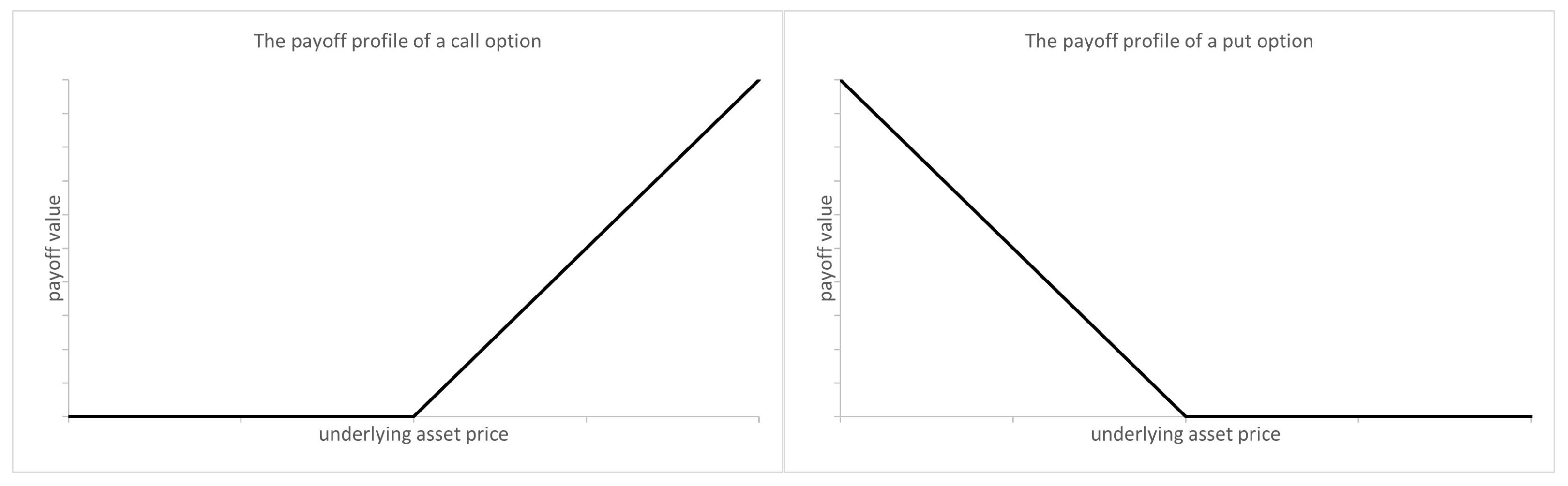
Definition A3. 
Acall optionis the right, but not the obligation, to buy a unit of the risky asset on a specified date, termed theexpiry dateof the option, at a price agreed at the time of origination of the option, termed thestrike price. Aput optionis the right, but not the obligation, to sell a unit of the risky asset on a specified date at a specified price [1].
In Appendix A, all options have an expiry date equal to the end point of the investment time period.
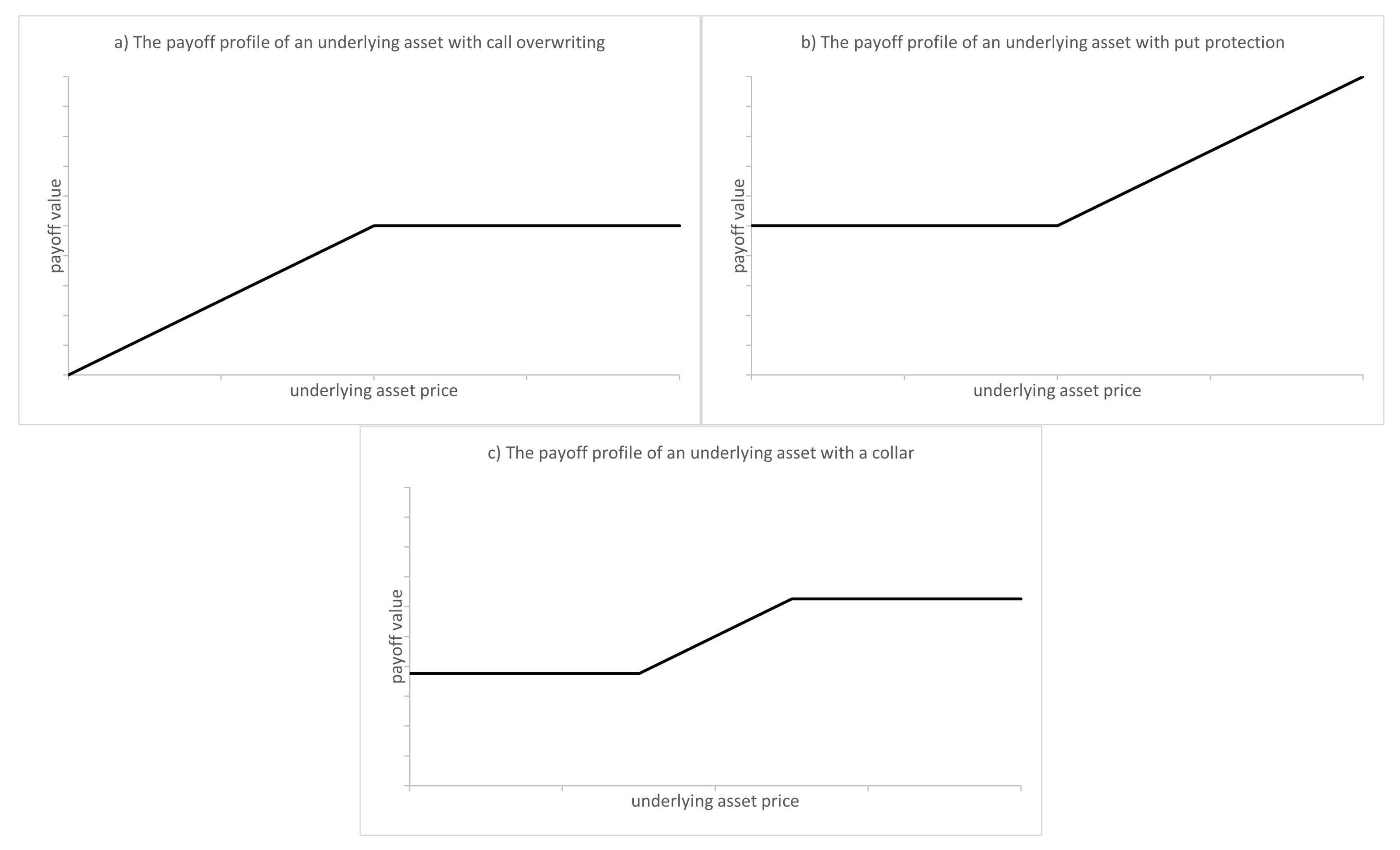
Definition A4. 
Aportfoliois a collection of assets and options [30]. An element of the portfolio is called aconstituent.
Multiple options can appear in a single portfolio, all potentially having different strike prices but all with the same expiry date. We will be specific about what is held in a portfolio, using statements such as ‘a portfolio consisting of the risk-free asset and a call option’, and where we need to be explicit, we will use the term option-adjusted portfolio to refer to a portfolio that contains options.
Definition A5. 
Avalue function, denoted in Appendix A by v ( . ) , is the value of an asset, option, or portfolio at the end of the time period, as a function of the underlying asset price, x.
It is commonly referred to as the payoff profile [18], but in Appendix A, we will use the term value function to reinforce the fact that it is a function of the asset price.
Property A1 
(Value of assets and options). The value functions of various assets are as follows:
For the risk-free asset, v ( x ) = x F [18]
For an asset, v ( x ) = x [18]
For a call option, v ( x ) = max ( x k , 0 ) where k denotes the strike price [18]
For a put option, v ( x ) = max ( k x , 0 ) where k denotes the strike price [1]
For an option-adjusted portfolio consisting of n p put options, with q i units of the ith put option which has strike price k i ( i = 1 , , n p ) , n c call options, with q i + n p units of the ith call option with strike price k i + n p ( i = 1 , , n c ) , q A units of the underlying asset, and q F invested in the risk-free asset, the value function is
v ( x ) = q F x F + q A x + i = 1 n p q i max ( k i x , 0 ) + i = n p + 1 n c q i max ( x k i , 0 )
Proof. 
By definition, the risk-free asset has a constant value at the end of the investment period and is not dependent on the risky asset. Therefore v ( x ) = x F for the risk-free asset.
The value of an investment in the risky asset is its price. Therefore v ( x ) = x for the risky asset.
If the risky asset price x is lower than the strike price k of a call option, then the option will not be exercised and expires worthless. Otherwise, the option is exercised, and the option owner can buy the risky asset at price k and immediately sell it at its price of x. Therefore v ( x ) = max ( x k , 0 ) for a call option.
Similarly, if the risky asset price is greater than the strike price of a put option, then the option expires worthless. Otherwise, the option is exercised, and the option owner can sell the risky asset at price k and immediately buy it back at price x. Therefore v ( x ) = max ( k x , 0 ) for a put option.
The value of a portfolio is the sum of the value of its constituents. The value of each constituent is the value of a single unit of each constituent multiplied by the number of units owned. Therefore, the portfolio value function is
v ( x ) = q F x F + q A x + i = 1 n p q i max ( k i x , 0 ) + i = n p + 1 n c q i max ( x k i , 0 )
Property A2 
(Put-call parity). A portfolio consisting of an underlying asset and a put option on that asset has the same value function as a portfolio consisting of a call option and an amount invested in the risk-free asset to buy the underlying asset if it were called [1].
Proof. 
A portfolio consisting of an underlying asset and a put option on that asset has a value function of max ( k x , 0 ) + x , where k denotes the strike price of the put, and x is the underlying asset price at expiry. This can be expressed as max ( k , x ) .
The amount needed to buy the underlying asset at the strike price on the expiry date must be k. Therefore a portfolio consisting of a call option and an amount invested in the risk-free asset to buy the underlying asset if it were called has a value function of max ( x k , 0 ) + k . This also can be expressed as max ( k , x ) . □
Definition A6. 
Anarbitrageexists if a portfolio with zero price has a non-negative value function (and the value function is strictly positive somewhere) [30].
Assumption A2. 
There are no arbitrage opportunities.
Property A3 
(Existence of option price). The price of both put and call options exist [31].
Proof. 
We focus on a put option first. We will show that its price is bounded above and below and therefore must exist.
No arbitrage ensures that there cannot exist a portfolio with zero starting value whose value function at expiry is positive for every price of the underlying asset.
Consider the portfolio consisting of a put option and a short position in the risk-free asset equal in size to the put option price. This portfolio has zero starting value. Its value function at expiry is v ( x ) = max ( k x , 0 ) p p u t x F s F , where p p u t denotes the price of the put option. If p p u t < 0 then v ( x ) > 0 for every value of x, which breaches the no arbitrage condition.
Consider now the reverse of this portfolio: a long position in the risk-free asset equal in size to the put option price, and a short put option. Its value function is v ( x ) = p p u t x F s F max ( k x , 0 ) . If p p u t > k / x F s F , then v ( x ) > 0 for every value of x which also breaches the no arbitrage condition. Therefore, p p u t is bounded and so must exist.
We now prove that a call option price exists. From the put-call parity property, the expiry value of a put option and the underlying asset equals the value of a call option and k / x F s F invested in the risk-free asset. Therefore p p u t + s = p c a l l + k / x F s F , where p c a l l denotes the price of the call option. Since s F and x F are finite quantities with x F strictly positive, and since we have shown that p p u t is bounded, then p c a l l is also bounded and therefore must also exist. □
Property A4 
(Sufficiency of call options). Every portfolio consisting of put and call options on an underlying asset, the underlying asset, and the risk-free asset can be expressed as a portfolio of solely call options, the underlying asset, and the risk-free asset.
Proof. 
This proof is based on put-call parity. The absence of arbitrage means that any two portfolios with the same value function must have the same price. Therefore, we need only demonstrate that the value function of any portfolio containing put options is equal to the value function of another portfolio not containing put options.
Let us suppose that the portfolio consists of n p put options, with q i units of the ith put option which has strike price k i ( i = 1 , , n p ) , n c call options, with q i + n p units of the ith call option with strike price k i + n p ( i = 1 , , n c ) , q A units of the underlying asset, and q F units of the risk-free asset.. The portfolio value function is
v ( x ) = q F x F + q A x + i = 1 n p q i max ( k i x , 0 ) + i = n p + 1 n c q i max ( x k i , 0 )
Now, max ( k i x , 0 ) = max ( x k i , 0 ) x + k i , and therefore we can write the value function as
v ( x ) = ( q F + 1 x F i = 1 n p q i k i ) x F + ( q A i = 1 n p q i max ( k i x , 0 ) ) x + i = 1 n c q i max ( x k i , 0 )
This is the value function of a portfolio consisting of solely call options, the underlying asset, and the risk-free asset. □
Definition A7. 
A function f ispiecewise linearon [ 0 , ) if for some partition 0 = x 0 < x 1 < < x m < x m + 1 = , it can be expressed as
f ( x ) = a i + b i ( x x i ) f o r   x i x < x i + 1 a n d   f o r i = 0 , , m
where a 0 , , a m and b 0 , , b m are finite constants [32]. (Note that the requirement that the constants are finite excludes vertical segments in the function).
Definition A8. 
A function f iscontinuousat ξ if lim x ξ f ( x ) = f ( ξ ) , and continuous everywhere if it is continuous at every point on its domain [32].
Definition A9. 
Acontinuous piecewise linear functionis a piecewise linear function that is continuous everywhere on its domain.
Property A5 
(Defining the intercepts of a continuous piecewise linear function). A function f is a continuous piecewise linear function on [ 0 , ) if, and only if, it can be expressed as
f ( x ) = a i + b i ( x x i ) f o r   x i x < x i + 1 and   for   i = 0 , , m
where a i = a i 1 + b i 1 ( x i x i 1 ) for i = 1 , , n .
Proof. 
By definition, if a function f is piecewise linear on [ 0 , ) , then it can be expressed as
f ( x ) = a i + b i ( x x i ) f o r   x i x < x i + 1 and   for   i = 0 , , m
If f is continuous everywhere, then in particular it is continuous at x i for i = 1 , , m . That implies that lim ϵ 0 f ( x i ϵ ) = f ( x i ) = a i . Now,
lim ϵ 0 f ( x i ϵ ) = lim ϵ 0 a i 1 + b i 1 ( x i ϵ x i 1 ) = a i 1 + b i 1 ( x i x i 1 )
Thus a i = a i 1 + b i 1 ( x i x i 1 ) as required.
Conversely, if f ( x ) = a i + b i ( x x i ) for x i x < x i + 1 and for i = 0 , , m where a i = a i 1 + b i 1 ( x i x i 1 ), then lim ϵ 0 f ( x i ϵ ) = f ( x i ) . Since the function is piecewise linear, and the domain of each segment includes the lower point of its partition, then lim ϵ 0 f ( x i + ϵ ) = f ( x i ) . Since lim ϵ 0 f ( x i ϵ ) = lim ϵ 0 f ( x i + ϵ ) , then lim x x i f ( x ) = f ( x i ) and therefore f is continuous at x i for i = 0 , , m . Furthermore, since all other points on the domain lie in the open interior of a line segment, f must be continuous at those points. Therefore, f is continuous everywhere as required. □
Property A6 
(Equivalence of the value of portfolios of options and continuous piecewise linear value functions). Every option-adjusted portfolio has a continuous piecewise linear value function, and every continuous piecewise linear function is the value function of some option-adjusted portfolio.
This property is a simple extension into the continuous domain of the well-known discrete case proven in [33].
Proof. 
First we prove that every option-adjusted portfolio has a continuous piecewise linear value function:
From the Sufficiency of Call Options Property, we can assume without loss of generality that the portfolio of options, the underlying asset, and the risk-free asset contains no puts, only calls. It therefore has a value function expressed as
v ( x ) = q F x F + q A x + i = 1 n q i max ( x x i , 0 )
where q F denotes the number of units of the risk-free asset owned, q A denotes the number of units of the underlying asset owned, n denotes the number of options, and q i denotes the number of units of the ith call option owned with strike price x i for i = 1 , , n . We order the n options such that x 1 < < x n and add x 0 = 0 and x n + 1 = enabling us to write that every x 0 satisfies x i x < x i + 1 for some i between 0 and n. Therefore, we can state that when x i x < x i + 1
i = 1 n q i max ( x x i , 0 ) = j = 1 i q j ( x x j )
This implies that when x i x < x i + 1
v ( x ) = q F x F + q A x + j = 1 i q j ( x x j ) = q F x F + q A x i + j = 1 i q j ( x i x j ) + ( q A + j = 1 i q j ) ( x x i )
By setting a i = q F x F + q A x i + j = 1 i q j ( x i x j ) and b i = q A + j = 1 i q j we can write that when x i x < x i + 1
v ( x ) = a i + b i ( x x i )
and since this expression for v ( x ) applies for x in every partition, we have shown that v is a piecewise linear function. Furthermore, for i = 1 , , n
a i = q F x F + q A x i + j = 1 i q j ( x i x j ) = a i 1 + ( q A + j = 1 i 1 q j ) ( x i x i 1 ) = a i 1 + b i 1 ( x i x i 1 )
This is the condition from the Defining the intercepts of a continuous piecewise linear function property, and therefore v is a continuous piecewise linear function.
Second, we prove that every continuous piecewise linear function is the value function of some option-adjusted portfolio:
By definition, if a function v is continuous and piecewise linear on [ 0 , ) then for some partition 0 = x 0 < x 1 < < x n < x n + 1 = , it can be expressed as
v ( x ) = a i + b i ( x x i ) for   x i x < x i + 1 and   for   i = 0 , , n
where a i = a i 1 + b i 1 ( x i x i 1 ) . From this recurrence relationship we can write that
a i = a 0 + j = 0 i 1 b j ( x j + 1 x j )
and so
v ( x ) = a 0 + j = 0 i 1 b j ( x j + 1 x j ) + b i ( x x i ) = a 0 j = 0 i b j x j + j = 0 i 1 b j x j + 1 + j = 0 i b j x j = 0 i 1 b j x = a 0 + b 0 x + j = 1 i ( b j b j 1 ) ( x x j )
However, since 0 = x 0 < x 1 < < x n < x n + 1 = , we know that
j = 1 i ( b j b j 1 ) ( x x j ) = i = 1 n ( b i b i 1 ) max ( x x i , 0 ) for   x i x < x i + 1
which means that
v ( x ) = a 0 + b 0 x + i = 1 n ( b i b i 1 ) max ( x x i , 0 ) for   all   x 0
This is the value function of an option-adjusted portfolio containing a 0 x F units of the risk-free asset, b 0 units of the underlying asset, and ( b i b i 1 ) units of a call option with strike price x i , where i = 1 , , n . □
Definition A10. 
Theinvestment returnis the change in value of the investment over the investment period as a proportion of the starting value [2].
The risk-free asset return is r F = x F s F 1 .
The risky asset return is r A = x s 1 .
The option-adjusted portfolio return is r O = v ( x ) s x F s F . p s + x F s F 1 where v ( x ) is the portfolio value function derived from the constituents of the portfolio, and p is the purchase price of the portfolio.
The intuition behind the option-adjusted portfolio return is that an investment is made in the risk-free asset, the price of the option portfolio is borrowed at the risk-free rate and used to purchase the option portfolio. Substituting the risk-free asset return allows us to rewrite r O as
r O = v ( x ) s ( 1 + r F ) p s + r F
The returns r A and r O are a function of the random variable x s which we shall label q. We shall denote the probability density function of q by g ( . ) .
Property A7 
(Mean and variance of an asset return). The expectation and variance of the risky asset return, E [ r A ] and V [ r A ] , respectively, (where E [ . ] denotes the expectation operator, and V [ . ] denotes the variance operator), are
E [ r A ] = Y 1 a n d V [ r A ] = Z Y 2
where Y = 0 q g ( q ) d q and Z = 0 q 2 g ( q ) d q
Proof. 
E [ r A ] = E [ x s ] 1 = Y 1 where Y = 0 q g ( q ) d q
V [ r A ] = E [ r A 2 ] E [ r A ] 2
E [ r A ] 2 = Y 2 2 Y 1
E [ r A 2 ] = E [ ( x s ) 2 ] 2 E [ x s ] 1 = Z 2 Y 1 where Z = 0 q 2 g ( q ) d q
Therefore V [ r A ] = Z 2 Y 1 ( Y 2 2 Y 1 ) = Z Y 2 . □
Property A8 
(Mean, variance, and covariance of an option-adjusted portfolio return). 
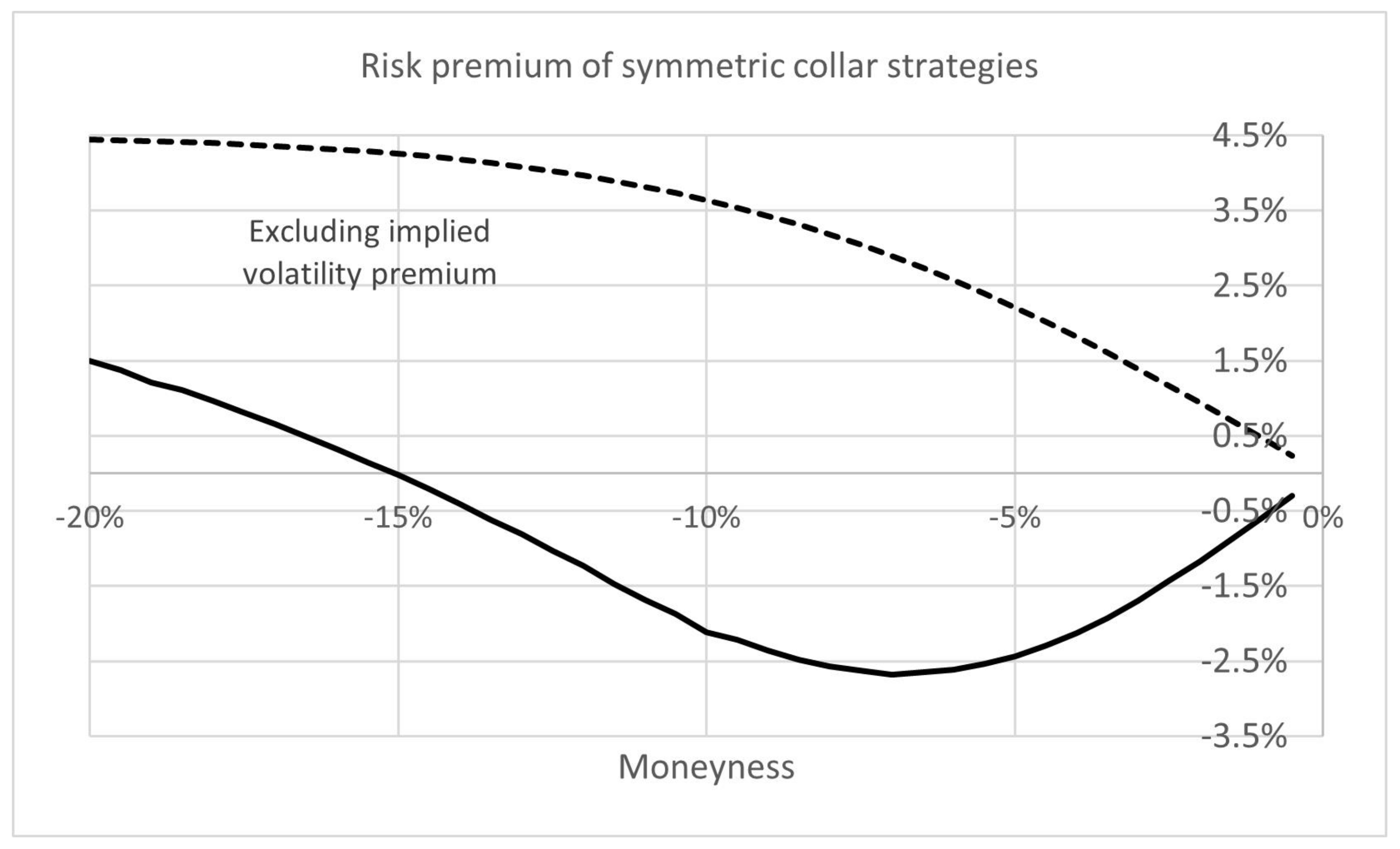
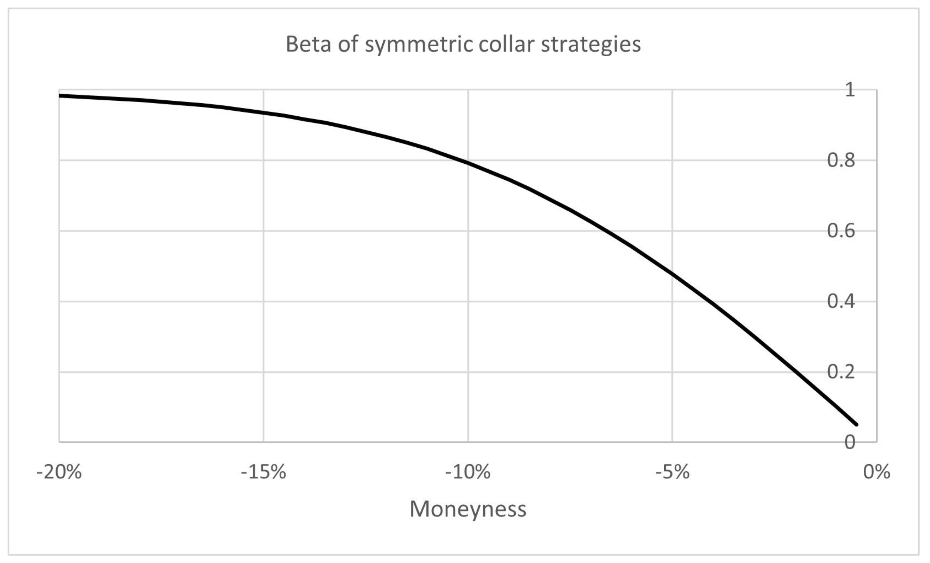
The return of an option-adjusted portfolio with a value function v ( x ) = a i + b i ( x x i ) for x i x < x i + 1 and for i = 0 , , n has expectation, variance, and covariance with risky asset return, as follows:
E [ r O ] = A + B ( 1 + r F ) p s + r F
where A = i = 0 n A i and B = i = 0 n B i , with A i = y i K i and B i = b i ( J i q i K i ) .
The variables y i and q i are defined as y i = a i s and q i = x i s for i = 0 , , n .
The variables K i and J i are defined as K i = q i q i + 1 g ( q ) d q and J i = q i q i + 1 q g ( q ) d q , for i = 0 , , n .
V [ r O ] = C + D + 2 E ( A + B ) 2
where C = i = 0 n C i , D = i = 0 n D i , and E = i = 0 n E i ,with C i = y i 2 L i , D i = b i 2 ( L i 2 q i J i + q i 2 K i ) , and E i = y i b i ( J i q i K i ) .
COV [ r O , r A ] = F + G Y ( A + B )
where F = i = 0 n F i and G = i = 0 n G i , with F i = y i J i and G i = b i ( L i q i J i ) .
The variable L i is defined as L i = q i q i + 1 q 2 g ( q ) d q , for i = 0 , , n .
Proof. 
From the value function we have that
v ( x ) s = y i + b i ( x s q i ) for   q i x s < q i + 1 and   for   i = 0 , , n
where for i = 0 , , n , y i = a i s and q i = x i s .
The first moment is written as
E v ( x ) s = q 0 q 1 ( y 0 + b 0 ( q q 0 ) ) g ( q ) d q + + q n q n + 1 ( y n + b n ( q q n ) ) g ( q ) d q = q 0 q 1 y 0 g ( q ) d q + + q n q n + 1 y n g ( q ) d q + q 0 q 1 b 0 ( q q 0 ) g ( q ) d q + + q n q n + 1 b n ( q q n ) g ( q ) d q = y 0 K 0 + y n K n + b 0 ( J 0 q 0 K 0 ) + + b n ( J n q n K n )
where K i = q i q i + 1 g ( q ) d q and J i = q i q i + 1 q g ( q ) d q , for i = 0 , , n . These can be considered as partitions of probability and expectation, respectively, in that i = 0 n K i = 1 and i = 0 n J i = Y .
By defining A i = y i K i and B i = b i ( J i q i K i ) , we can say
E v ( x ) s = i = 0 n A i + i = 0 n B i
Finally, letting A = i = 0 n A i and B = i = 0 n B i we have that
E v ( x ) s = A + B
Therefore
E [ r O ] = E v ( x ) s ( 1 + r F ) p s + r F = A + B ( 1 + r F ) p s + r F
Similarly, the second moment is written as
E v ( x ) s 2 = q 0 q 1 ( y 0 + b 0 ( q q 0 ) ) 2 g ( q ) d q + + q n q n + 1 ( y n + b n ( q q n ) ) ) 2 g ( q ) d q = q 0 q 1 y 0 2 g ( q ) d q + + q n q n + 1 y n 2 g ( q ) d q + q 0 q 1 b 0 2 ( q q 0 ) 2 g ( q ) d q + + q n q n + 1 b n 2 ( q q n ) 2 g ( q ) d q + 2 q 0 q 1 y 0 b 0 ( q q n ) g ( q ) d q + + q n q n + 1 y 0 b n ( q q n ) g ( q ) d q = i = 0 n C i + i = 0 n D i + 2 i = 0 n E i
where C i = q i q i + 1 y i 2 g ( q ) d q , D i = q i q i + 1 b i 2 ( q q i ) 2 g ( q ) d q and E i = q i q i + 1 y i b i ( q q i ) g ( q ) d q .
We can immediately write that C i = y i 2 K i and E i = y i b i ( J i q i K i ) for i = 0 , , n .
For D 0 , , D n we expand the squared term of the integrand giving us that D i = q i q i + 1 b i 2 ( q 2 2 q q i + q i 2 ) g ( q ) d q . Defining L i = q i q i + 1 q 2 g ( q ) d q (which can be considered as a partition of the second moment satisfying i = 0 n L i = Z ), we can write that, for i = 0 , , n , D i = b i 2 ( L i 2 q i J i + q i 2 K i ) .
Finally, letting C = i = 0 n C i , D = i = 0 n D i and E = i = 0 n E i , we have that
E v ( x ) s 2 = C + D + 2 E
Combining these two expressions gives us that
V [ r O ] = V v ( x ) s = E v ( x ) s 2 E v ( x ) s 2 = C + D + 2 E ( A + B ) 2
In addition,
E v ( x ) s . x s = q 0 q 1 ( y 0 + b 0 ( q q 0 ) ) q 2 g ( q ) d q + + q n q n + 1 ( y n + b n ( q q n ) ) q 2 g ( q ) d q = q 0 q 1 y 0 q g ( q ) d q + + q n q n + 1 y n q g ( q ) d q + q 0 q 1 b 0 ( q q 0 ) q g ( q ) d q + + q n q n + 1 b n ( q q n ) q g ( q ) d q = i = 0 n F i + i = 0 n G i
where F i = q i q i + 1 y i q g ( q ) d q and G i = q i q i + 1 b i ( q q i ) q g ( q ) d q . Using the above definitions, we write F i = y i J i and G i = b i ( L i q i J i ) . Letting F = i = 0 n F i and G = i = 0 n G i
E v ( x ) s . x s = F + G
Therefore
COV [ r O , r / ! A ] = E v ( x ) s . x s E v ( x ) s E x s = F + G Y ( A + B )
as required. □
Property A9 
(Statistics under geometric Brownian motion). When the underlying asset price follows a geometric Brownian motion process with instantaneous mean μ, and instantaneous standard deviation σ, then
Y = exp { μ t } a n d Z = exp { ( 2 μ + σ 2 ) t }
where t denotes the length of time of the investment period, and
K i = Φ ( u i + 1 ) Φ ( u i ) J i = Y ( Φ ( v i + 1 ) Φ ( v i ) ) L i = Z ( Φ ( w i + 1 ) Φ ( w i ) )
where
u i = log ( q i ) ( μ 1 / 2 σ 2 ) t σ t v i = log ( q i ) ( μ + 1 / 2 σ 2 ) t σ t w i = log ( q i ) ( μ + 3 / 2 σ 2 ) t σ t
Proof. 
If the asset price follows geometric Brownian motion with instantaneous mean μ , and instantaneous standard deviation σ , then q, is log-normally distributed. Specifically log ( q ) is normally distributed with mean θ = ( μ 1 / 2 σ 2 ) t and variance ω 2 = σ 2 t .
Letting y = ( log ( q ) θ ) / ω we can write
K i = q i q i + 1 g ( q ) d q = u i u i + 1 1 2 π exp { 1 / 2 y 2 } d y
where u i = ( log ( q i ) θ ) / ω , which can be expressed as
u i = log ( q i ) θ ω = log ( q i ) ( μ 1 / 2 σ 2 ) t σ t
Therefore, K i = Φ ( u i + 1 ) Φ ( u i )
where Φ ( z ) is the cumulative distribution function of a standard normal distribution. That is
Φ ( z ) = z 1 2 π exp { 1 / 2 y 2 } d y
Similarly,
J i = q i q i + 1 q g ( q ) d q = u i u i + 1 exp { y ω + θ } 1 2 π exp { 1 / 2 y 2 } d y = exp { 1 / 2 ω 2 + θ } u i u i + 1 1 2 π exp { 1 / 2 ( y ω ) 2 } d y
Letting z = y ω , we can write
J i = exp { 1 / 2 ω 2 + θ } v i v i + 1 1 2 π exp { 1 / 2 z 2 } d z
where v i = u i ω . which can be expressed as
v i = log ( q i ) ( μ + 1 / 2 σ 2 ) t σ t
Noting that exp { 1 / 2 ω 2 + θ } = exp { μ t } , and using identical logic to the above, we also have that
Y = 0 q g ( q ) d q = exp { 1 / 2 ω 2 + θ } 1 2 π exp { 1 / 2 z 2 } d z = exp { μ t }
Therefore, J i = Y ( Φ ( v i + 1 ) Φ ( v i ) ) .
Similarly,
L i = q i q i + 1 q 2 g ( q ) d q = u i u i + 1 exp { y ω + θ } 2 1 2 π exp { 1 / 2 y 2 } d y = exp { 2 ω 2 + 2 θ } u i u i + 1 1 2 π exp { 1 / 2 ( y 2 ω ) 2 } d y
Letting z = y 2 ω , we can write
L i = exp { 2 ω 2 + 2 θ } w i w i + 1 1 2 π exp { 1 / 2 z 2 } d z
where w i = u i 2 ω , which can be expressed as
w i = u i 2 ω = log ( q i ) ( μ + 3 / 2 σ 2 ) t σ t
Noting that exp { 2 ω 2 + 2 θ } = exp { ( 2 μ + σ 2 ) t } , and using identical logic to the above, we also have that
Z = 0 q 2 g ( q ) d q = exp { 2 ω 2 + 2 θ } 1 2 π exp { 1 / 2 z 2 } d z = exp { ( 2 μ + σ 2 ) t }
Therefore, L i = Z ( Φ ( w i + 1 ) Φ ( w i ) ) . □
Definition A11. 
Theinstantaneous risk-free rate, denoted by r f , satisfies r f = 1 t log ( 1 + r F ) .
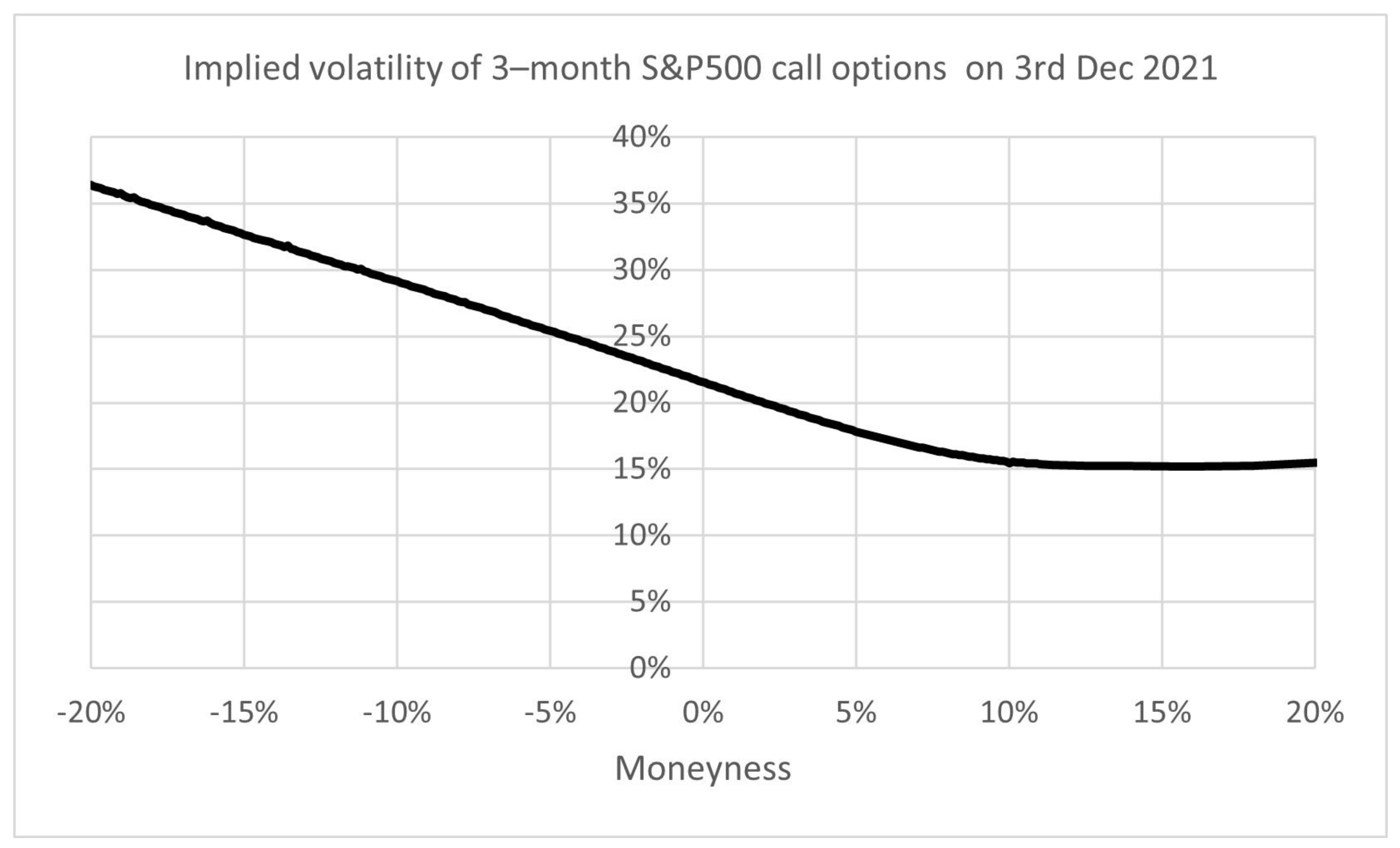
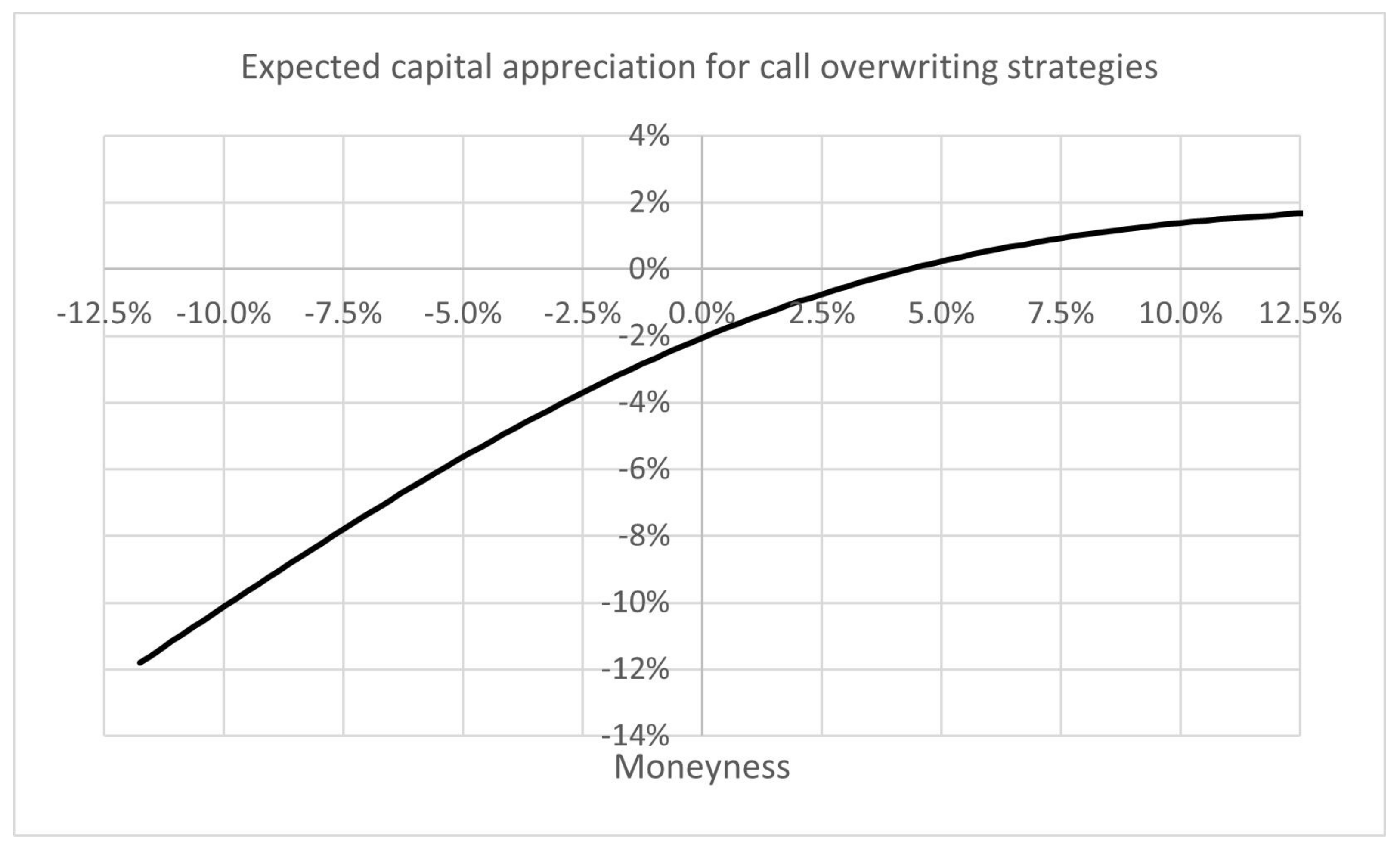
Property A10 
(Option price under geometric Brownian motion). When the underlying asset price follows a geometric Brownian motion process with instantaneous mean μ, and instantaneous standard deviation σ, then ( 1 + r F ) p s = A * + B * where A * and B * are computed exactly as A and B were described in the Mean, variance, and covariance of an option-adjusted portfolio return property, but with μ replaced throughout by the instantaneous risk-free rate r f and σ by the implied volatility of the call option with the ith strike price.
Proof. 
If the asset price follows a geometric Brownian motion process, then a risk-neutral portfolio can be formed [1]. Therefore, the options can be priced using risk-neutral valuation with the market’s price of volatility. Mathematically, this is expressed as
( 1 + r F ) p s = E * v ( x ) s
where the E * [ . ] represents the expectation operator using the risk-neutral distribution. Under the risk-neutral distribution log ( q ) is normally distributed with mean ( r f 1 / 2 σ * 2 ) t and variance σ * 2 t , where σ * denotes the implied volatility. Following the logic of the Mean, variance, and covariance of an option-adjusted portfolio return property, we can write that
E * v ( x ) s = i = 0 n A i * + i = 0 n B i *
where A i * = y i K i * and B i * = b i ( J i * q i K i * ) , for i = 0 , , n , and
K i * = q i q i + 1 g ( q ) d q a n d J i * = q i q i + 1 q g ( q ) d q .
Furthermore, we can use the statistics under geometric Brownian motion property to say
K i * = Φ ( u i + 1 * ) Φ ( u i * ) J i * = Y * ( Φ ( v i + 1 * ) Φ ( v i * ) )
where
u i * = log ( q i ) ( r f 1 / 2 σ * 2 ) t σ * t v i * = log ( q i ) ( r f + 1 / 2 σ * 2 ) t σ * t
with Y * = exp { r f t } . □
Property A11 
(Covariance of one option-adjusted asset with another asset). The return of an option-adjusted asset (with a value function, v ( 1 ) , defined by intercepts y 1 ( 1 ) , , y n ( 1 ) , slopes b 1 ( 1 ) , , b n ( 1 ) , and strikes q 1 ( 1 ) , , q n ( 1 ) on an underlying asset with start and end prices of s ( 1 ) and x ( 1 ) , respectively) have a covariance with the return of another, non-option adjusted, asset (with start and end prices of s ( 2 ) and x ( 2 ) , respectively) given by
COV [ r O ( 1 ) , r A ( 2 ) ] = E v ( 1 ) ( x ( 1 ) ) s ( 1 ) . x ( 2 ) s ( 2 ) E v ( 1 ) ( x ( 1 ) ) s ( 1 ) E x ( 2 ) s ( 2 )
where
E v ( 1 ) ( x ( 1 ) ) s ( 1 ) . x ( 2 ) s ( 2 ) = D + E
where D = i = 0 n D i and E = i = 0 n E i
with D i = b i ( 1 ) ( L i q i ( 1 ) J i ) and E i = y i ( 1 ) J i for i = 0 , , n .
J i = Y ( 2 ) ( Φ ( ψ i + 1 ) Φ ( ψ i ) ) L i = Y ( 12 ) ( Φ ( ξ i + 1 ) Φ ( ξ i ) )
where
ψ i = log ( q i ( 1 ) ) ( μ ( 1 ) 1 / 2 ( σ ( 1 ) 2 2 ρ σ ( 1 ) σ ( 2 ) ) ) t σ ( 1 ) t ξ i = log ( q i ( 1 ) ) ( μ ( 1 ) + 1 / 2 ( σ ( 1 ) 2 + 2 ρ σ ( 1 ) σ ( 2 ) ) ) t σ ( 1 ) t
and where Y ( 1 ) = exp { μ ( 1 ) t } , Y ( 2 ) = exp { μ ( 2 ) t } , and Y ( 12 ) = Y ( 1 ) Y ( 2 ) exp { ρ σ ( 1 ) σ ( 2 ) t } .
The variables μ ( 1 ) and σ ( 1 ) denote the instantaneous mean and standard deviation of the price process of the underlying asset in the option-adjusted asset, and μ ( 2 ) and σ ( 2 ) denote the instantaneous mean and standard deviation of the price process of the other asset, and ρ denotes their instantaneous correlation.
Proof. 
The option-adjusted asset has value function denoted by v ( 1 ) . Its return is
r O ( 1 ) = v ( 1 ) ( x ( 1 ) ) s ( 1 ) ( 1 + r F ) p ( 1 ) s ( 1 ) + r F
Therefore
r O ( 1 ) E [ r O ( 1 ) ] = v ( 1 ) ( x ( 1 ) ) s ( 1 ) E v ( 1 ) ( x ( 1 ) ) s ( 1 )
The covariance of this return with another asset is therefore
COV [ r O ( 1 ) , r A ( 2 ) ] = E r O ( 1 ) E [ r O ( 1 ) ] r A ( 2 ) E [ r A ( 2 ) ] = E v ( 1 ) ( x ( 1 ) ) s ( 1 ) E v ( 1 ) ( x ( 1 ) ) s ( 1 ) x ( 2 ) s ( 2 ) E x ( 2 ) s ( 2 ) = E v ( 1 ) ( x ( 1 ) ) s ( 1 ) . x ( 2 ) s ( 2 ) E v ( 1 ) ( x ( 1 ) ) s ( 1 ) E x ( 2 ) s ( 2 )
Now,
E v ( 1 ) ( x ( 1 ) ) s ( 1 ) . x ( 2 ) s ( 2 ) = q 0 ( 1 ) q 1 ( 1 ) 0 ( y 0 ( 1 ) + b 0 ( 1 ) ( q ( 1 ) q 0 ( 1 ) ) ) q ( 2 ) g ( q ( 1 ) , q ( 2 ) ) d q ( 2 ) d q ( 1 ) + + q n ( 1 ) q n + 1 ( 1 ) 0 ( y n ( 1 ) + b n ( 1 ) ( q ( 1 ) q n ( 1 ) ) ) q ( 2 ) g ( q ( 1 ) , q ( 2 ) ) d q ( 2 ) d q ( 1 ) = i = 0 n y i ( 1 ) J i + i = 0 n b i ( 1 ) ( L i q i ( 1 ) J i )
where
J i = q i ( 1 ) q i + 1 ( 1 ) 0 q ( 2 ) g ( q ( 1 ) , q ( 2 ) ) d q ( 2 ) d q ( 1 ) L i = q i ( 1 ) q i + 1 ( 1 ) 0 q ( 1 ) q ( 2 ) g ( q ( 1 ) , q ( 2 ) ) d q ( 2 ) d q ( 1 )
We can express this as
E v ( 1 ) ( x ( 1 ) ) s ( 1 ) . x ( 2 ) s ( 2 ) = D + E
where D = i = 0 n D i and E = i = 0 n E i with D i = b i ( 1 ) ( L i q i ( 1 ) J i ) and E i = y i ( 1 ) J i .
If q ( 1 ) and q ( 2 ) follow the bivariate the geometric Brownian motion process defined by
d q ( 1 ) = q ( 1 ) μ ( 1 ) d t + q ( 1 ) σ ( 1 ) d W ( 1 ) d q ( 2 ) = q ( 2 ) μ ( 2 ) d t + q ( 2 ) σ ( 2 ) ( ρ d W ( 1 ) + γ d W ( 2 ) )
where γ = 1 ρ 2 , then, for k = 1   and   2 , log ( q ( k ) ) is distributed normally with mean θ ( k ) and variance ω ( k ) 2 , with correlation ρ , where
θ ( k ) = ( μ ( k ) 1 / 2 σ ( k ) 2 ) t and ω ( k ) = σ ( k ) t
In this case we have that
J i = q i ( 1 ) q i + 1 ( 1 ) 0 q ( 2 ) g ( q ( 1 ) , q ( 2 ) ) d q ( 2 ) d q ( 1 ) = u i ( 1 ) u i + 1 ( 1 ) 0 exp { ω ( 2 ) y ( 2 ) + θ ( 2 ) } × 1 2 π γ exp { 1 2 γ 2 ( y ( 1 ) 2 2 ρ y ( 1 ) y ( 2 ) + y ( 2 ) 2 ) } d y ( 2 ) d y ( 1 ) = Y ( 2 ) u i ( 1 ) u i + 1 ( 1 ) 1 2 π exp { 1 / 2 ( y ( 1 ) ρ ω ( 2 ) ) 2 } d y ( 1 )
where
u i ( 1 ) = log ( q i ( 1 ) ) ( μ ( 1 ) M M 1 / 2 σ ( 1 ) 2 ) t σ ( 1 ) t
and where Y ( 2 ) = exp { μ ( 2 ) t } .
Let z = y ( 1 ) ρ ω ( 2 ) , then
J i = Y ( 2 ) ψ i ( 1 ) ψ i + 1 ( 1 ) 1 2 π exp { 1 / 2 z 2 } d z
where ψ i ( 1 ) = u i ( 1 ) ρ ω ( 2 ) , which can be expressed as
ψ i ( 1 ) = u i ( 1 ) ω ( 1 ) = log ( q i ( 1 ) ) ( μ ( 1 ) 1 / 2 ( σ ( 1 ) 2 2 ρ σ ( 1 ) σ ( 2 ) ) ) t σ ( 1 ) t
Therefore, J i = Y ( 2 ) ( Φ ( ψ i + 1 ( 1 ) ) Φ ( ψ i ( 1 ) ) ) .
We also have that
L i = q i ( 1 ) q i + 1 ( 1 ) 0 q ( 1 ) q ( 2 ) g ( q ( 1 ) , q ( 2 ) ) d q ( 2 ) d q ( 1 ) = u i ( 1 ) u i + 1 ( 1 ) 0 exp { ω ( 1 ) y ( 1 ) + θ ( 1 ) } e x p { ω ( 2 ) y ( 2 ) + θ ( 2 ) } × 1 2 π γ exp { 1 2 γ 2 ( y ( 1 ) 2 2 ρ y ( 1 ) y ( 2 ) + y ( 2 ) 2 ) } d y ( 2 ) d y ( 1 ) = Y ( 12 ) u i ( 1 ) u i + 1 ( 1 ) 1 2 π exp { 1 / 2 ( y ( 1 ) ( ρ ω ( 2 ) + ω ( 1 ) ) ) 2 } d y ( 1 )
where Y ( 12 ) = Y ( 1 ) Y ( 2 ) exp { ρ σ ( 1 ) σ ( 2 ) t } .
Let z = y ( 1 ) ω ( 1 ) ρ ω ( 2 ) , then
L i = Y ( 12 ) ξ i ( 1 ) ξ i + 1 ( 1 ) 1 2 π exp { 1 / 2 z 2 ) } d z
where ξ i ( 1 ) = u i ( 1 ) ω ( 1 ) ρ ω ( 2 ) , which can be expressed as
ξ i ( 1 ) = u i ( 1 ) ω ( 1 ) ρ ω ( 2 ) = log ( q i ( 1 ) ) ( μ ( 1 ) + 1 / 2 ( σ ( 1 ) 2 + 2 ρ σ ( 1 ) σ ( 2 ) ) ) t σ ( 1 ) t
Therefore, L i = Y ( 12 ) ( Φ ( ξ i + 1 ( 1 ) ) Φ ( ξ i ( 1 ) ) )
Property A12 
(Covariance of two option-adjusted assets). Consider two option-adjusted assets. The first has a value function, v ( 1 ) , defined by intercepts y 1 ( 1 ) , , y n ( 1 ) ( 1 ) , slopes b 1 ( 1 ) , , b n ( 1 ) ( 1 ) , and strikes q 1 ( 1 ) , , q n ( 1 ) ( 1 ) , on an underlying asset with start and end prices of s ( 1 ) and x ( 1 ) , respectively. The second has a value function defined by has a value function, v ( 2 ) , defined by intercepts y 1 ( 2 ) , , y n ( 2 ) ( 2 ) , slopes b 1 ( 2 ) , , b n ( 2 ) ( 2 ) , and strikes q 1 ( 1 ) , , q n ( 2 ) ( 2 ) on an underlying asset with start and end prices of s ( 2 ) and x ( 2 ) , respectively.
The covariance of returns of two option-adjusted assets is
COV [ r O ( 1 ) , r O ( 2 ) ] = E v ( 1 ) ( x ( 1 ) ) s ( 1 ) . v ( 2 ) ( x ( 2 ) ) s ( 2 ) E v ( 1 ) ( x ( 1 ) ) s ( 1 ) E v ( 2 ) ( x ( 2 ) ) s ( 2 )
where
E v ( 1 ) ( x ( 1 ) ) s ( 1 ) . v ( 2 ) ( x ( 2 ) ) s ( 2 ) = C + D + E 1 + E 2
where C = i = 0 n ( 1 ) j = 0 n ( 2 ) C i j , D = i = 0 n ( 1 ) j = 0 n ( 2 ) D i j , E 1 = i = 0 n ( 1 ) j = 0 n ( 2 ) E 1 i j , and E 2 = i = 0 n ( 1 ) j = 0 n ( 2 ) E 2 i j with
C i j = y i ( 1 ) y j ( 2 ) K i j D i j = b i ( 1 ) b j ( 2 ) ( L i i q j ( 2 ) J i j ( 1 ) q i ( 1 ) J i j ( 2 ) + q i ( 1 ) q j ( 2 ) K i j ) E 1 i j = y i ( 1 ) b j ( 2 ) ( J i j ( 2 ) q j ( 2 ) K i j ) E 2 i j = y j ( 2 ) b i ( 1 ) ( J i j ( 1 ) q i ( 1 ) K i j )
and
K i j = Φ ρ ( u i + 1 ( 1 ) , u j + 1 ( 2 ) ) Φ ρ ( u i + 1 ( 1 ) , u j ( 2 ) ) Φ ρ ( u i ( 1 ) , u j + 1 ( 2 ) ) + Φ ρ ( u i ( 1 ) , u j ( 2 ) ) J i j ( 1 ) = Y ( 1 ) ( Φ ρ ( v i + 1 ( 1 ) , ψ j + 1 ( 2 ) ) Φ ρ ( v i + 1 ( 1 ) , ψ j ( 2 ) ) Φ ρ ( v i ( 1 ) , ψ j + 1 ( 2 ) ) + Φ ρ ( v i ( 1 ) , ψ j ( 2 ) ) ) J i j ( 2 ) = Y ( 2 ) ( Φ ρ ( ψ i + 1 ( 1 ) , v j + 1 ( 2 ) ) Φ ρ ( ψ i + 1 ( 1 ) , v j ( 2 ) ) Φ ρ ( ψ i ( 1 ) , v j + 1 ( 2 ) ) + Φ ρ ( ψ i ( 1 ) , v j ( 2 ) ) ) L i j = Y ( 12 ) ( Φ ρ ( ξ i + 1 ( 1 ) , ξ j + 1 ( 2 ) ) Φ ρ ( ξ i + 1 ( 1 ) , ξ j ( 2 ) ) Φ ρ ( ξ i ( 1 ) , ξ j + 1 ( 2 ) ) + Φ ρ ( ξ i ( 1 ) , ξ j ( 2 ) ) )
where for k = 1   a n d   2 ,
ψ i ( k ) = log ( q i ( k ) ) ( μ ( k ) 1 / 2 ( σ ( k ) 2 2 ρ σ ( 1 ) σ ( 2 ) ) ) t σ ( k ) t ξ i ( k ) = log ( q i ( k ) ) ( μ ( k ) + 1 / 2 ( σ ( k ) 2 + 2 ρ σ ( 1 ) σ ( 2 ) ) ) t σ ( k ) t
and Y ( 1 ) = exp { μ ( 1 ) t } , Y ( 2 ) = exp { μ ( 2 ) t } and Y ( 12 ) = Y ( 1 ) Y ( 2 ) exp { ρ σ ( 1 ) σ ( 2 ) t } .
The function Φ ρ ( x , y ) is the cumulative distribution function of the bivariate standard normal distribution with correlation ρ.
The variables μ ( 1 ) and σ ( 1 ) denote the instantaneous mean and standard deviation of the price process of the underlying asset in the option-adjusted asset, and μ ( 2 ) and σ ( 2 ) denote the instantaneous mean and standard deviation of the price process of the other asset, and ρ denotes their instantaneous correlation.
Proof. 
For asset k ( k = 1   and   2 ), the option-adjusted return is
r O ( k ) = v ( k ) ( x ( k ) ) s ( k ) ( 1 + r F ) p ( k ) s ( k ) + r F
Therefore
r O ( k ) E [ r O ( k ) ] = v ( k ) ( x ( k ) ) s ( k ) E v ( k ) ( x ( k ) ) s ( k )
The covariance of these returns is therefore
COV [ r O ( 1 ) , r O ( 2 ) ] = E ( r O ( 1 ) E [ r O ( 1 ) ] ) ( r O ( 2 ) E [ r O ( 2 ) ] ) = E v ( 1 ) ( x ( 1 ) ) s ( 1 ) E v ( 1 ) ( x ( 1 ) ) s ( 1 ) v ( 2 ) ( x ( 2 ) ) s ( 2 ) E v ( 2 ) ( x ( 2 ) ) s ( 2 ) = E v ( 1 ) ( x ( 1 ) ) s ( 1 ) . v ( 2 ) ( x ( 2 ) ) s ( 2 ) E v ( 1 ) ( x ( 1 ) ) s ( 1 ) E v ( 2 ) ( x ( 2 ) ) s ( 2 )
Now,
E v ( 1 ) ( x ( 1 ) ) s ( 1 ) . v ( 2 ) ( x ( 2 ) ) s ( 2 ) = q 0 ( 1 ) q 1 ( 1 ) q 0 ( 2 ) q 1 ( 2 ) y 0 ( 1 ) + b 0 ( 1 ) ( q ( 1 ) q 0 ( 1 ) ) y 0 ( 2 ) + b 0 ( 2 ) ( q ( 2 ) q 0 ( 2 ) ) g ( q ( 1 ) , q ( 2 ) ) d q ( 2 ) d q ( 1 ) + + q n ( 1 ) ( 1 ) q n ( 2 ) ( 2 ) y n ( 1 ) ( 1 ) + b n ( 1 ) ( 1 ) ( q ( 1 ) q n ( 1 ) ( 1 ) ) y n ( 2 ) ( 2 ) + b n ( 2 ) ( 2 ) ( q ( 2 ) q n ( 2 ) ( 2 ) ) g ( q ( 1 ) , q ( 2 ) ) d q ( 2 ) d q ( 1 ) = i = 0 n ( 1 ) j = 0 n ( 2 ) y i ( 1 ) y j ( 2 ) K i j + i = 0 n ( 1 ) j = 0 n ( 2 ) y i ( 1 ) b j ( 2 ) ( J i j ( 2 ) q j ( 2 ) K i j ) + i = 0 n ( 1 ) j = 0 n ( 2 ) y j ( 2 ) b i ( 1 ) ( J i j ( 1 ) q i ( 1 ) K i j ) + i = 0 n ( 1 ) j = 0 n ( 2 ) b i ( 1 ) b j ( 2 ) ( L i j q j ( 2 ) J i j ( 1 ) q i ( 1 ) J i j ( 2 ) + q i ( 1 ) q j ( 2 ) K i j )
where
K i j = q i ( 1 ) q i + 1 ( 1 ) q j ( 2 ) q j + 1 ( 2 ) g ( q ( 1 ) , q ( 2 ) ) d q ( 2 ) d q ( 1 ) J i j ( 1 ) = q i ( 1 ) q i + 1 ( 1 ) q j ( 2 ) q j + 1 ( 2 ) q ( 1 ) g ( q ( 1 ) , q ( 2 ) ) d q ( 2 ) d q ( 1 ) J i j ( 2 ) = q i ( 1 ) q i + 1 ( 1 ) q j ( 2 ) q j + 1 ( 2 ) q ( 2 ) g ( q ( 1 ) , q ( 2 ) ) d q ( 2 ) d q ( 1 ) L i j = q i ( 1 ) q i + 1 ( 1 ) q j ( 2 ) q j + 1 ( 2 ) q ( 1 ) q ( 2 ) g ( q ( 1 ) , q ( 2 ) ) d q ( 2 ) d q ( 1 )
We can express this as
E v ( 1 ) ( x ( 1 ) ) s ( 1 ) . v ( 2 ) ( x ( 2 ) ) s ( 2 ) = C + D + E 1 + E 2
where C = i = 0 n ( 1 ) j = 0 n ( 2 ) C i j , D = i = 0 n ( 1 ) j = 0 n ( 2 ) D i j , E 1 = i = 0 n ( 1 ) j = 0 n ( 2 ) E 1 i j , and E 2 = i = 0 n ( 1 ) j = 0 n ( 2 ) E 2 i j with
C i j = y i ( 1 ) y j ( 2 ) K i j D i j = b i ( 1 ) b j ( 2 ) ( L i i q j ( 2 ) J i j ( 1 ) q i ( 1 ) J i j ( 2 ) + q i ( 1 ) q j ( 2 ) K i j ) E 1 i j = y i ( 1 ) b j ( 2 ) ( J i j ( 2 ) q j ( 2 ) K i j ) E 2 i j = y j ( 2 ) b i ( 1 ) ( J i j ( 1 ) q i ( 1 ) K i j )
If q ( 1 ) and q ( 2 ) follow the bivariate of the geometric Brownian motion process defined by
d q ( 1 ) = q ( 1 ) μ ( 1 ) d t + q ( 1 ) σ ( 1 ) d W ( 1 ) d q ( 2 ) = q ( 2 ) μ ( 2 ) d t + q ( 2 ) σ ( 2 ) ( ρ d W ( 1 ) + γ d W ( 2 ) )
where γ = 1 ρ 2 , then, for k = 1   and   2 , log ( q ( k ) ) is distributed normally with mean θ ( k ) and variance ω ( k ) 2 , with correlation ρ , where
θ ( k ) = ( μ ( k ) 1 / 2 σ ( k ) 2 ) t and ω ( k ) = σ ( k ) t
In this case we have that
K i j = q i ( 1 ) q i + 1 ( 1 ) q j ( 2 ) q j + 1 ( 2 ) g ( q ( 1 ) , q ( 2 ) ) d q ( 1 ) d q ( 2 ) = u i ( 1 ) u i + 1 ( 1 ) u j ( 2 ) u j + 1 ( 2 ) 1 2 π γ exp { 1 2 γ 2 ( z ( 1 ) 2 2 ρ z ( 1 ) z ( 2 ) + z ( 2 ) 2 ) } d z ( 1 ) d z ( 2 )
where u i ( k ) = ( log ( q i ( k ) ) θ ( k ) ) / ω ( k ) , which can be expressed as
u i ( k ) = log ( q i ( k ) ) ( μ ( k ) M M 1 / 2 σ ( k ) 2 ) t σ ( k ) t
Therefore
K i j = Φ ρ ( u i + 1 ( 1 ) , u j + 1 ( 2 ) ) Φ ρ ( u i + 1 ( 1 ) , u j ( 2 ) ) Φ ρ ( u i ( 1 ) , u j + 1 ( 2 ) ) + Φ ρ ( u i ( 1 ) , u j ( 2 ) )
where Φ ρ ( x , y ) is the cumulative distribution function of the bivariate standard normal distribution with correlation ρ . That is
Φ ρ ( x , y ) = x y 1 2 π γ exp { 1 2 γ 2 ( x 2 2 ρ x y + y 2 ) } d x d y
J i j ( 1 ) = q i ( 1 ) q i + 1 ( 1 ) q j ( 2 ) q j + 1 ( 2 ) q ( 1 ) g ( q ( 1 ) , q ( 2 ) ) d q ( 2 ) d q ( 1 ) = u i ( 1 ) u i + 1 ( 1 ) u j ( 2 ) u j + 1 ( 2 ) exp { ω ( 1 ) y ( 1 ) + θ ( 1 ) } × 1 2 π γ exp { 1 2 γ 2 ( y ( 1 ) 2 2 ρ y ( 1 ) y ( 2 ) + y ( 2 ) 2 ) } d y ( 2 ) d y ( 1 )
Let z ( 1 ) = y ( 1 ) ω ( 1 ) and z ( 2 ) = y ( 2 ) ρ ω ( 2 ) , then
J i j ( 1 ) = exp { θ ( 1 ) + 1 2 ω ( 1 ) 2 } × v i ( 1 ) v i + 1 ( 1 ) ψ j ( 2 ) ψ j + 1 ( 2 ) 1 2 π γ exp { 1 2 γ 2 ( z ( 1 ) 2 2 ρ z ( 1 ) z ( 2 ) + z ( 2 ) 2 ) } d z ( 1 ) d z ( 2 )
where v i ( 1 ) = u i ( 1 ) ω ( 1 ) and ψ j ( 2 ) = u j ( 2 ) ρ ω ( 1 ) , which can be expressed as
v i ( 1 ) = log ( q i ( 1 ) ) ( μ ( 1 ) + 1 / 2 σ ( 1 ) 2 ) t σ ( 1 ) t ψ i ( 2 ) = log ( q i ( 2 ) ) ( μ ( 2 ) 1 / 2 ( σ ( 2 ) 2 2 ρ σ ( 1 ) σ ( 2 ) ) ) t σ ( 2 ) t
Therefore
J i j ( 1 ) = Y ( 1 ) Φ ρ ( v i + 1 ( 1 ) , ψ j + 1 ( 2 ) ) Φ ρ ( v i + 1 ( 1 ) , ψ j ( 2 ) ) Φ ρ ( v i ( 1 ) , ψ j + 1 ( 2 ) ) + Φ ρ ( v i ( 1 ) , ψ j ( 2 ) )
where Y ( 1 ) = exp { μ ( 1 ) t } .
Similarly,
J i j ( 2 ) = Y ( 2 ) Φ ρ ( ψ i + 1 ( 1 ) , v j + 1 ( 2 ) ) Φ ρ ( ψ i + 1 ( 1 ) , v j ( 2 ) ) Φ ρ ( ψ i ( 1 ) , v j + 1 ( 2 ) ) + Φ ρ ( ψ i ( 1 ) , v j ( 2 ) )
where Y ( 2 ) = exp { μ ( 2 ) t } and
v i ( 2 ) = log ( q i ( 2 ) ) ( μ ( 2 ) + 1 / 2 σ ( 2 ) 2 ) t σ ( 2 ) t ψ i ( 1 ) = log ( q i ( 1 ) ) ( μ ( 1 ) 1 / 2 ( σ ( 1 ) 2 2 ρ σ ( 1 ) σ ( 2 ) ) ) t σ ( 1 ) t
L i j = q i ( 1 ) q i + 1 ( 1 ) q j ( 2 ) q j + 1 ( 2 ) q ( 1 ) q ( 2 ) g ( q ( 1 ) , q ( 2 ) ) d q ( 2 ) d q ( 1 ) = u i ( 1 ) u i + 1 ( 1 ) u j ( 2 ) u j + 1 ( 2 ) exp { ω ( 1 ) y ( 1 ) + θ ( 1 ) } exp { ω ( 2 ) y ( 2 ) + θ ( 2 ) } × 1 2 π γ exp { 1 2 γ 2 ( y ( 1 ) 2 2 ρ y ( 1 ) y ( 2 ) + y ( 2 ) 2 ) } d y ( 2 ) d y ( 1 )
Let z ( 1 ) = y ( 1 ) ω ( 1 ) ρ ω ( 2 ) and z ( 2 ) = y ( 2 ) ω ( 2 ) ρ ω ( 1 ) , then
L i j = exp { θ ( 1 ) + θ ( 2 ) + 1 2 ( ω ( 1 ) 2 + 2 ρ ω ( 1 ) ω ( 2 ) + ω ( 2 ) 2 ) } × ξ i ( 1 ) ξ i + 1 ( 1 ) ξ j ( 2 ) ξ j + 1 ( 2 ) 1 2 π γ exp { 1 2 γ 2 ( z ( 1 ) 2 2 ρ z ( 1 ) z ( 2 ) + z ( 2 ) 2 ) } d z ( 1 ) d z ( 2 )
where ξ i ( 1 ) = u i ( 1 ) ω ( 1 ) ρ ω ( 2 ) and ξ j ( 2 ) = u j ( 2 ) ω ( 2 ) ρ ω ( 1 ) , which can be expressed as
ξ i ( k ) = log ( q i ( k ) ) ( μ ( k ) + 1 / 2 ( σ ( k ) 2 + 2 ρ σ ( 1 ) σ ( 2 ) ) ) t σ ( k ) t
Therefore
L i j = Y ( 12 ) Φ ρ ( ξ i + 1 ( 1 ) , ξ j + 1 ( 2 ) ) Φ ρ ( ξ i + 1 ( 1 ) , ξ j ( 2 ) ) Φ ρ ( ξ i ( 1 ) , ξ j + 1 ( 2 ) ) + Φ ρ ( ξ i ( 1 ) , ξ j ( 2 ) )
where Y ( 12 ) = Y ( 1 ) Y ( 2 ) exp { ρ σ ( 1 ) σ ( 2 ) t } . □
Property A13 
(Existence of moments of a value function). If E [ r A ] and V [ r A ] exist, then E [ r O ] and V [ r O ] exist.
Proof. 
Since the probability density function of asset return, g ( ) , is positive everywhere, 0 K i 0 g ( q ) d q , 0 J i 0 q g ( q ) d q , and 0 L i 0 q 2 g ( q ) d q . By definition 0 g ( q ) d q = 1 , so for i = 0 , , n , K i is bounded and therefore must exist. Furthermore, if the mean and variance of the underlying asset exist, then 0 q g ( q ) d q and 0 q 2 g ( q ) d q also exist and therefore J i and L i are bounded for i = 0 , , n and so must exist.
From the Mean, variance, and covariance of an option-adjusted portfolio return property we know that E [ v ( x ) s ] and V [ v ( x ) s ] are quadratic functions of K i , J i , and L i for i = 0 , , n and therefore must exist. Since V [ r O ] = V [ v ( x ) s ] , V [ r O ] also exists.
We have shown that any option-adjusted portfolio is a combination of the risk-free asset, the risky asset, and a set of call options. We have further shown that the price of every call option exists, and therefore the price of the option strategy, p, must also exist. Since E [ r O ] = E [ v ( x ) s ] x F s F . p s + x F s F 1 , and x F exists, and s F > 0 , E [ r O ] must also exist. □
Definition A12. 
An option-adjusted portfolio (with a non-negative initial price) isunleveragedif the value of the portfolio at the end of the time-period is non-negative everywhere.
Property A14 
(unleveraged option-adjusted portfolio condition). An option-adjusted portfolio is unleveraged if, and only if, v m = min ( v ( x ) ) exists and p v m / ( 1 + r F ) + s .
Proof. 
The end value of an option-adjusted portfolio is v ( x ) p ( 1 + r F ) + s ( 1 + r F ) .
If v ( x ) has a minimum, v m , and if p v m / ( 1 + r F ) + s then v m p ( 1 + r F ) + s ( 1 + r F ) 0 and since v ( x ) v m , v ( x ) p ( 1 + r F ) + s ( 1 + r F ) 0 for all x. Therefore, the portfolio is unleveraged.
If the portfolio is unleveraged then v ( x ) p ( 1 + r F ) + s ( 1 + r F ) 0 for all x. Therefore, v ( x ) p ( 1 + r F ) s ( 1 + r F ) . Since p is finite, v ( x ) must have a minimum. Furthermore v m p ( 1 + r F ) + s ( 1 + r F ) 0 and therefore v m / ( 1 + r F ) + s p . □
Definition A13. 
An unleveraged option-adjusted portfolio iswell-behavedif v ( x ) / ( 1 + r F ) + s = p only when x = 0 .
Property A15 
(Existence of log moments of a value function). If E [ r A ] and V [ r A ] exist, and E [ log ( 1 + r A ) ] and V [ log ( 1 + r A ) ] exist, then E [ log ( 1 + r O ) ] and V [ log ( 1 + r O ) ] also exist for a well-behaved unleveraged portfolio.
Proof. 
Recall that r O = v ( q s ) s p s ( 1 + r F ) + r F where q = x s . Since log ( z ) < z 1 for all z > 0 we can write
E [ log ( 1 + r O ) ] = 0 log v ( q s ) s p s ( 1 + r F ) + ( 1 + r F ) g ( q ) d q < 0 v ( q s ) s p s ( 1 + r F ) + r F g ( q ) d q = E [ R O ]
E [ log ( 1 + r O ) 2 ] = 0 log v ( q s ) s p s ( 1 + r F ) + ( 1 + r F ) 2 g ( q ) d q < 0 v ( q s ) s p s ( 1 + r F ) + r F 2 g ( q ) d q = E [ R O 2 ]
Using the Existence of moments of a value function property, E [ R O ] and E [ R O 2 ] exist. Therefore, these upper bounds exist.
E [ log ( 1 + r O ) ] = 0 log v ( q s ) p s ( 1 + r F ) + ( 1 + r F ) g ( q ) d q = 0 q 1 log v ( q s ) p s ( 1 + r F ) + ( 1 + r F ) g ( q ) d q + q 1 log v ( q s ) p s ( 1 + r F ) + ( 1 + r F ) g ( q ) d q
Since the portfolio is leveraged and well-behaved, v ( q s ) p ( 1 + r F ) + s ( 1 + r F ) > 0 for all q > 0 and q 1 > 0 ,
log v ( q s ) p s ( 1 + r F ) + ( 1 + r F ) > for   all   q > q 1
and so
0 log v ( q s ) p s ( 1 + r F ) + ( 1 + r F ) >
When q q 1 , v ( q s ) = a 0 + b 0 q s , therefore 1 + r O = y 0 + b 0 q p s ( 1 + r F ) + ( 1 + r F ) when q q 1 (where y 0 = a 0 s ). Moreover, since v ( q s ) p ( 1 + r F ) + s ( 1 + r F ) 0 for all q 0 ,
y 0 p s ( 1 + r F ) + ( 1 + r F ) 0
which means 1 + r O b 0 q s when q q 1 . Therefore
0 q 1 log v ( q s ) p s ( 1 + r F ) + ( 1 + r F ) g ( q ) d q log ( b 0 s ) 0 q 1 g ( q ) d q + 0 q 1 log ( q ) g ( q ) d q .
Since E [ log ( 1 + r A ) ] exists, both of these integrals exist. Therefore
0 q 1 log ( ( v ( q s ) p s ( 1 + r F ) + ( 1 + r F ) ) g ( q ) d q >
Thus E [ log ( 1 + r O ) ] > .
Finally, since log ( x ) 2 0 for all x, E [ log ( 1 + R O ) 2 ] 0 .
Since E [ log ( 1 + R O ) ] and E [ log ( 1 + R O ) 2 ] are bounded above and below, they must exist. Therefore E [ log ( 1 + R O ) ] and V [ log ( 1 + R O ) ] exist. □
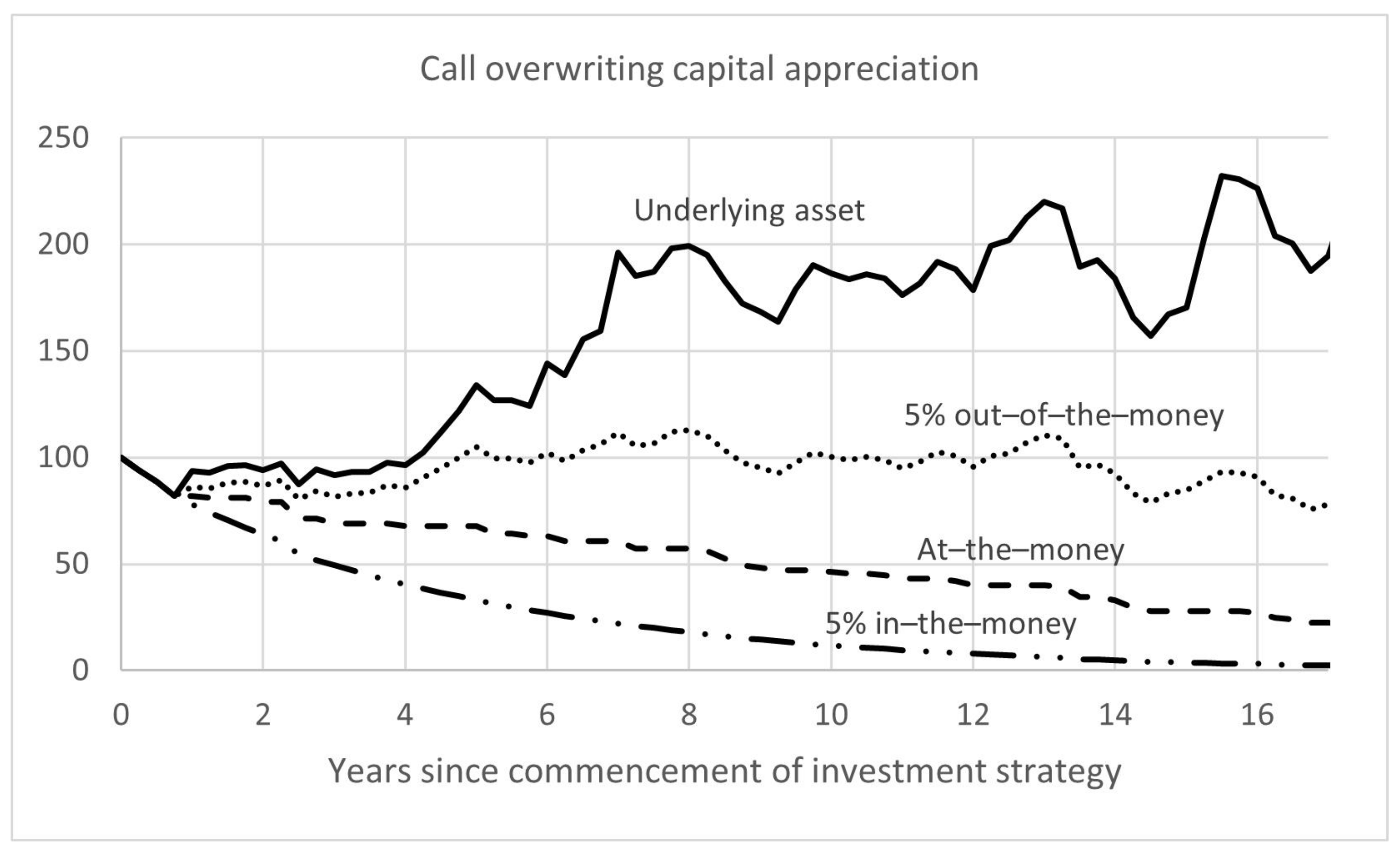
In the remainder of this Appendix we shall be considering long-run returns of option-adjusted portfolios and will view these portfolios as a sequence of m single-period option strategies. We will let r A ( 1 ) , , r A ( m ) denote the single-period returns for the underlying asset, and let r O ( 1 ) , , r O ( m ) denote the single-period returns for the option-adjusted portfolio. The value functions of the options strategies in each single-period are denoted by v ( 1 ) ( x ) , , v ( m ) ( x ) . Furthermore, we will let p ( 1 ) , , p ( m ) denote the option-adjusted portfolio prices, s ( 1 ) , , s ( m ) denote the prices of the underlying asset at the start of the single periods, and x ( 1 ) , , x ( m ) denote the prices of the underlying asset at the end of the single-periods.
Property A16 
(Independence of option-adjusted portfolio returns). If r A ( 1 ) , , r A ( m ) are mutually independent random variables, then r O ( 1 ) , , r O ( m ) are mutually independent.
Proof. 
For i = 1 , , m ,
r A ( i ) = x ( i ) s ( i ) 1 a n d r O ( i ) = v ( i ) ( x ( i ) ) s ( i ) ( 1 + r F ) p ( i ) s ( i ) + r F
Therefore
r O ( i ) = v ( i ) ( s ( i ) ( 1 + r A ( i ) ) ) s ( i ) ( 1 + r F ) p ( i ) s ( i ) + r F
Since each r O ( i ) is a function solely of the random variable r A ( i ) , if r A ( 1 ) , , r A ( m ) are mutually independent then r O ( 1 ) , , r O ( m ) must also be mutually independent. □
Definition A14. 
Two option strategies, deployed at different points in time, areidenticalif
1.
the initial amounts in invested in the risk-free rate are the same proportions of the starting underlying asset prices; and
2.
the number of units invested in the underlying asset are the same; and
3.
the number of options are the same; and
4.
every pair of corresponding options in the two strategies has the same moneyness.
If every pair of option strategies in a sequence over time are identical, then the option-adjusted portfolio is said to beinvariant.
Property A17 
(Proportional value functions). If two option strategies are identical then their value functions, v ( 1 ) and v ( 2 ) , satisfy v ( 1 ) ( s ( 1 ) x ) s ( 1 ) = v ( 2 ) ( s ( 2 ) x ) s ( 2 ) for all x.
Proof. 
If the two strategies are identical then their value functions are expressed as
v ( 1 ) ( x ) = q F ( 1 ) s F ( 1 ) ( 1 + r F ) + q A x + i = 1 n q i max ( x x ( 1 ) i , 0 ) v ( 2 ) ( x ) = q F ( 2 ) s F ( 2 ) ( 1 + r F ) + q A x + i = 1 n q i max ( x x ( 2 ) i , 0 )
Therefore
v ( 1 ) ( s ( 1 ) x ) s ( 1 ) = q F ( 1 ) s F ( 1 ) s ( 1 ) ( 1 + r F ) + q A x + i = 1 n q i max ( x x ( 1 ) i s ( 1 ) , 0 ) v ( 2 ) ( s ( 2 ) x ) s ( 2 ) = q F ( 2 ) s F ( 2 ) s ( 2 ) ( 1 + r F ) + q A x + i = 1 n q i max ( x x ( 2 ) i s ( 2 ) , 0 )
but since they are identical, q F ( 1 ) s F ( 1 ) s ( 1 ) = q F ( 2 ) s F ( 2 ) s ( 2 ) and the same moneyness means that x ( 1 ) i s ( i ) = x ( 2 ) i s ( 2 ) for i = 1 , , n , therefore v ( 1 ) ( s ( 1 ) x ) s ( 1 ) = v ( 2 ) ( s ( 2 ) x ) s ( 2 ) . □
Property A18 
(Identicality of option-adjusted returns). If r A ( 1 ) , , r A ( m ) are identically distributed, then r O ( 1 ) , , r O ( m ) are identically distributed for invariant option-adjusted portfolios.
Proof. 
For i = 0 , , n , and for any real-valued y, define the subset of the real numbers, Ω ( i ) ( y ) , as
Ω ( i ) ( y ) = z : v ( i ) ( s ( i ) z ) s ( i ) ( 1 + r F ) p ( i ) s ( i ) + r F < y .
Since r A ( 1 ) , , r A ( m ) are identically distributed, so are 1 + r A ( 1 ) , , 1 + r A ( m ) . We will label 1 + r A ( i ) as X. Then we can write that for i = 1 , , m
r O ( i ) = v ( i ) ( s ( i ) X ) s ( i ) ( 1 + r F ) p ( i ) s ( i ) + r F
Therefore, P ( r O ( i ) < y ) = Ω ( i ) ( y ) π ( x ) d x where π ( x ) is the probability density function of X. But for an invariant option-adjusted portfolio, v ( i ) ( s ( i ) x ) s ( i ) = v ( j ) ( s ( j ) x ) s ( j ) , and the absence of arbitrage means that p ( i ) s ( i ) = p ( j ) s ( j ) for any i and j. Therefore Ω ( i ) ( y ) = Ω ( j ) ( y ) for all y and any i and j, and so P ( r O ( i ) < y ) = P ( r O ( j ) < y ) . Thus r O ( i ) and r O ( j ) are identical. □
Definition A15. 
For a portfolio (or asset) with value u ( i ) at time i (for i = 0 , , m ), itsannualised long run-returnis
u ( m ) u ( 0 ) 1 m 1
Property A19 
(Chain linked returns). The annualised long-run log return of a portfolio (or asset) is the average of the single-period log returns.
Proof. 
u ( m ) u ( 0 ) 1 m = u ( 1 ) u ( 0 ) × × u ( m ) u ( m 1 ) 1 m = ( 1 + r ( 1 ) ) × × ( 1 + r ( m ) ) 1 m
where r ( 1 ) , , r ( m ) denote the m single-period returns.
Therefore
log u ( m ) u ( 0 ) 1 m = log ( 1 + r ( 1 ) ) + + log ( 1 + r ( m ) ) m
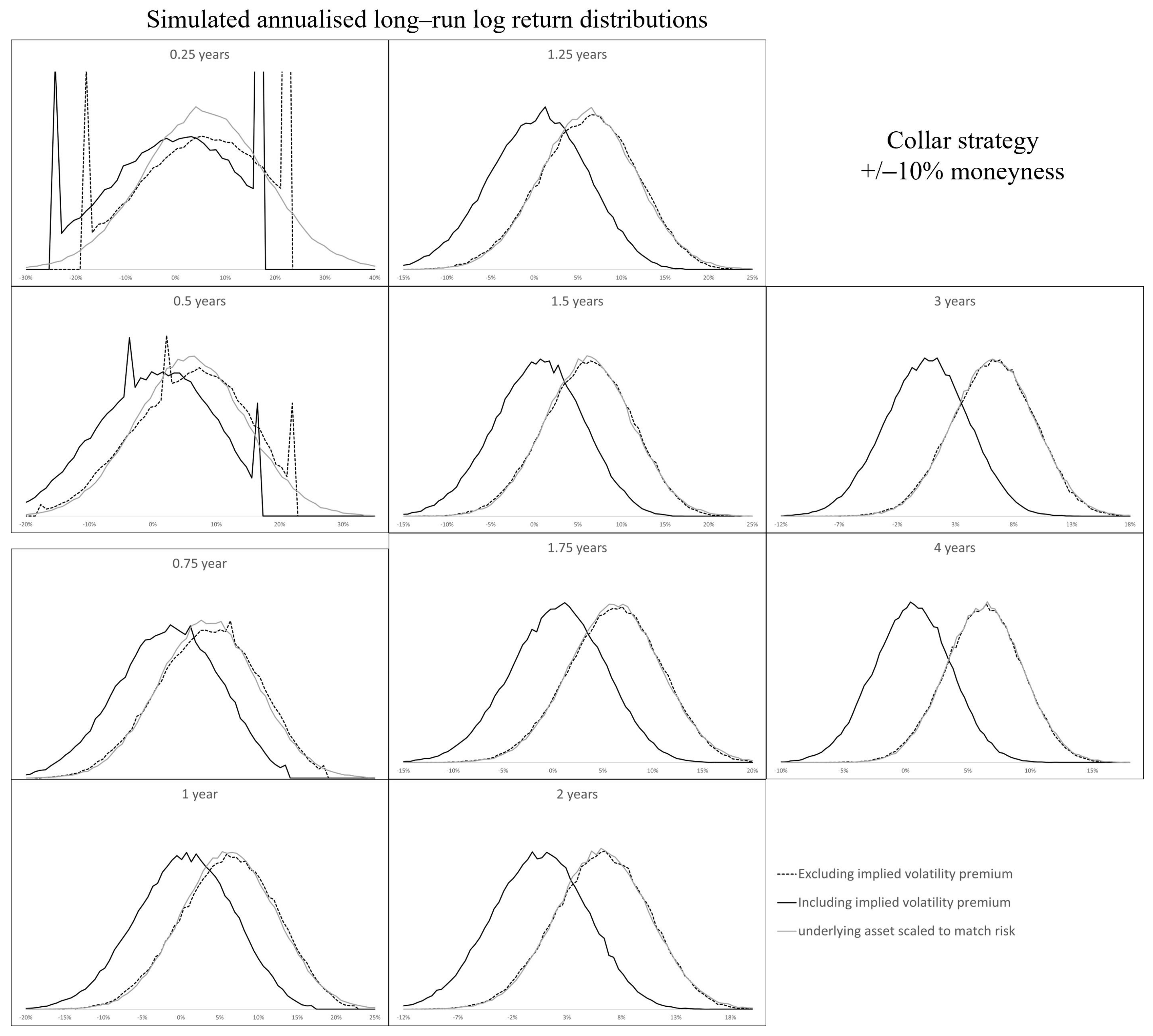
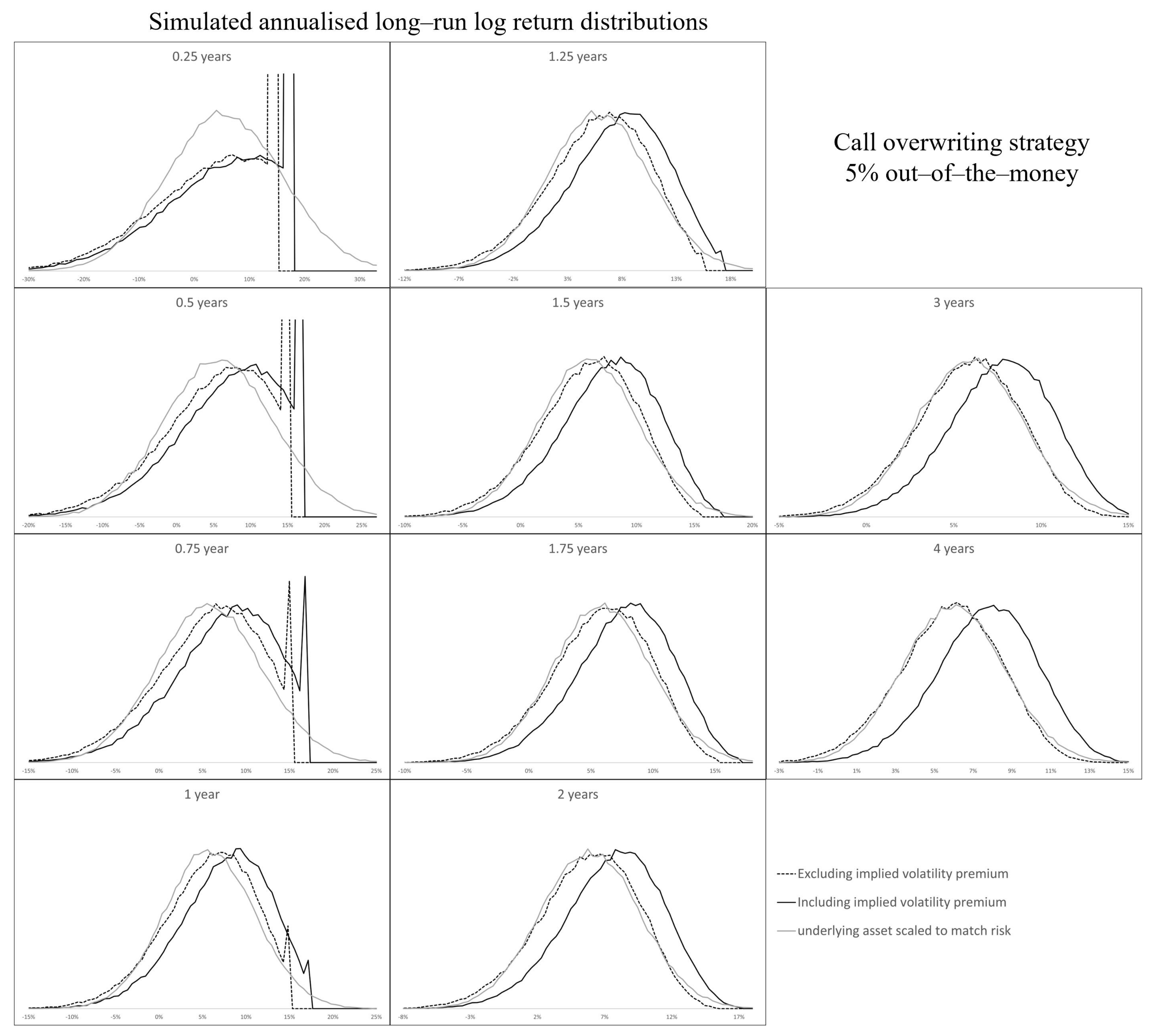
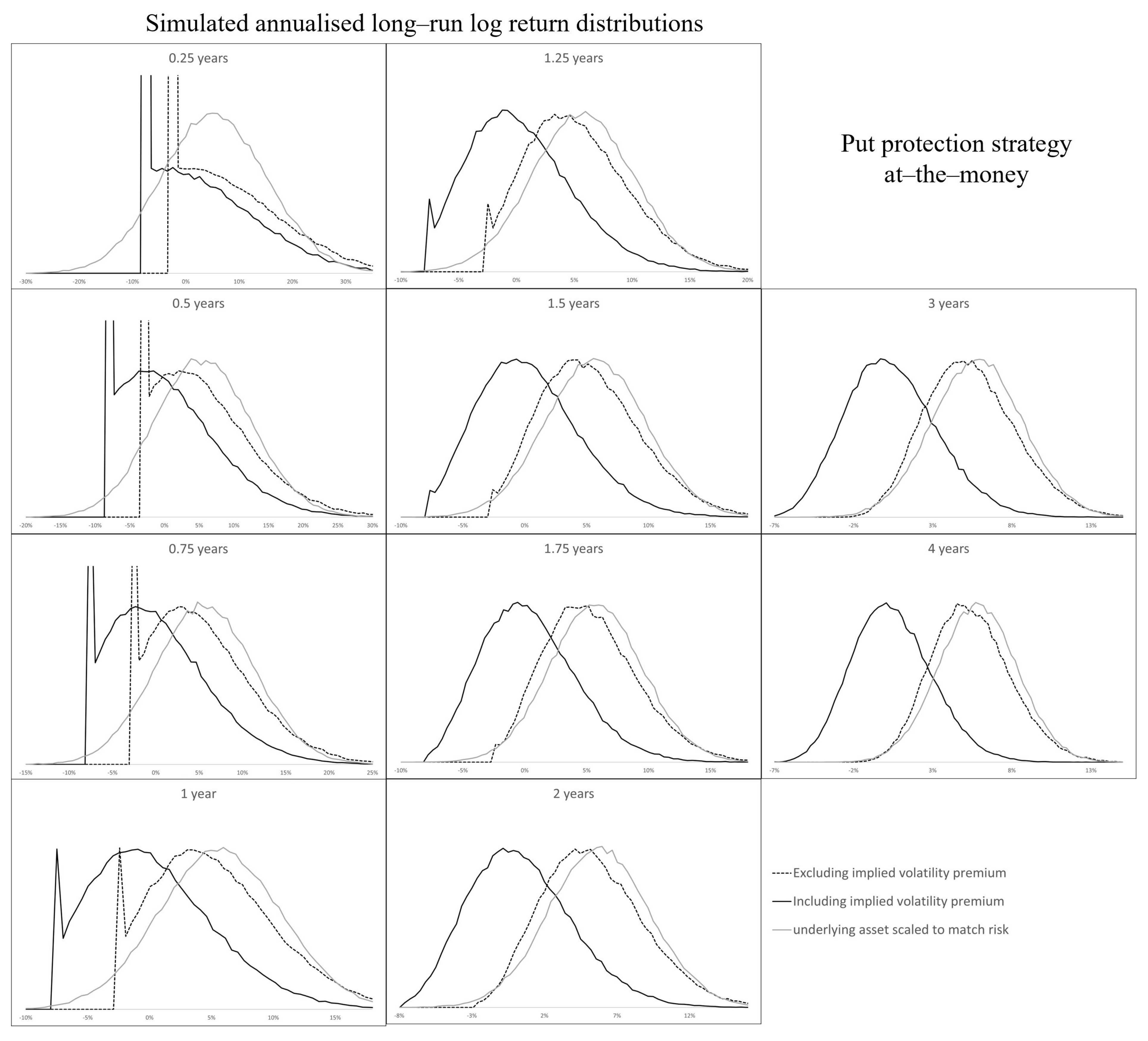
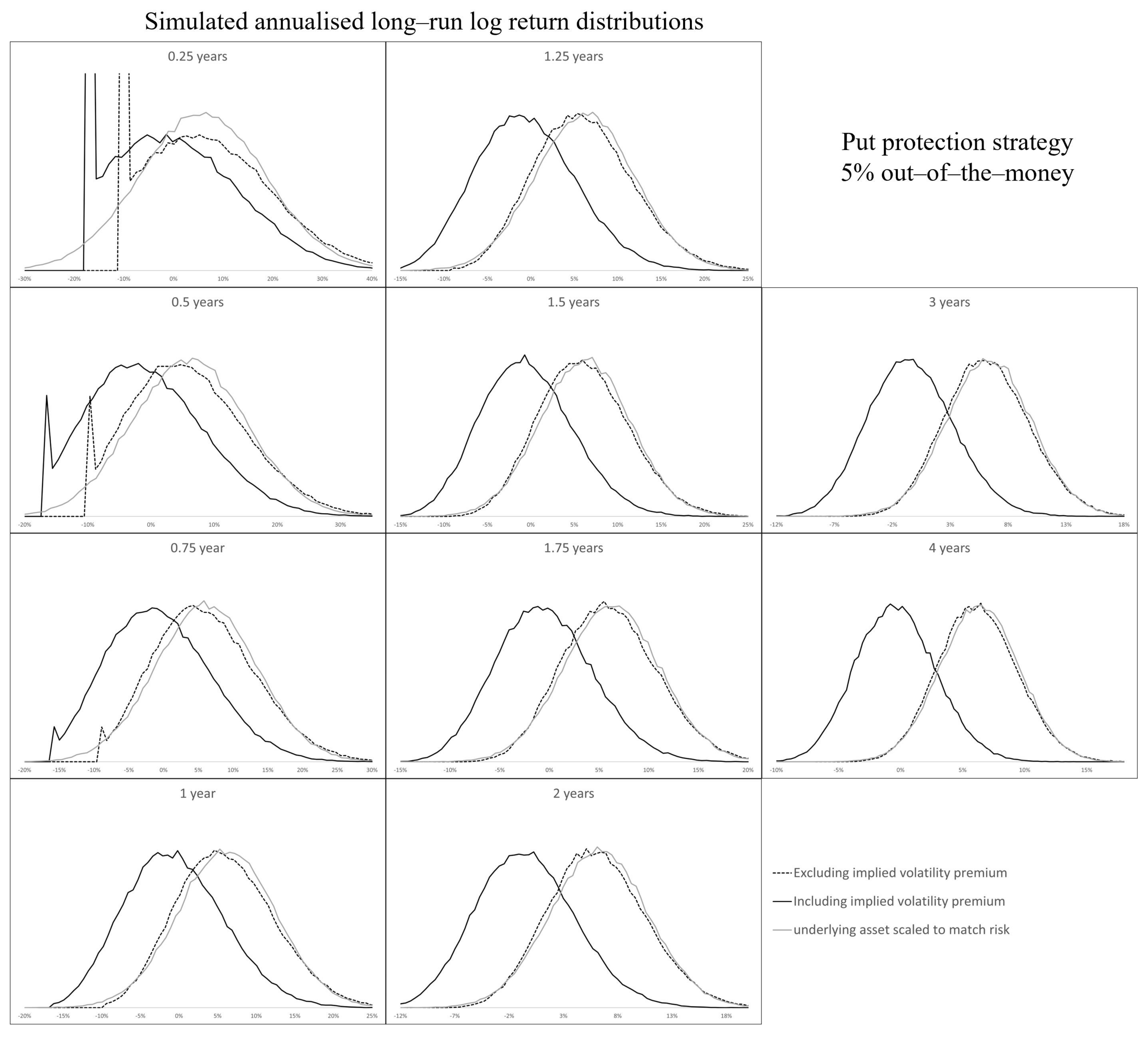
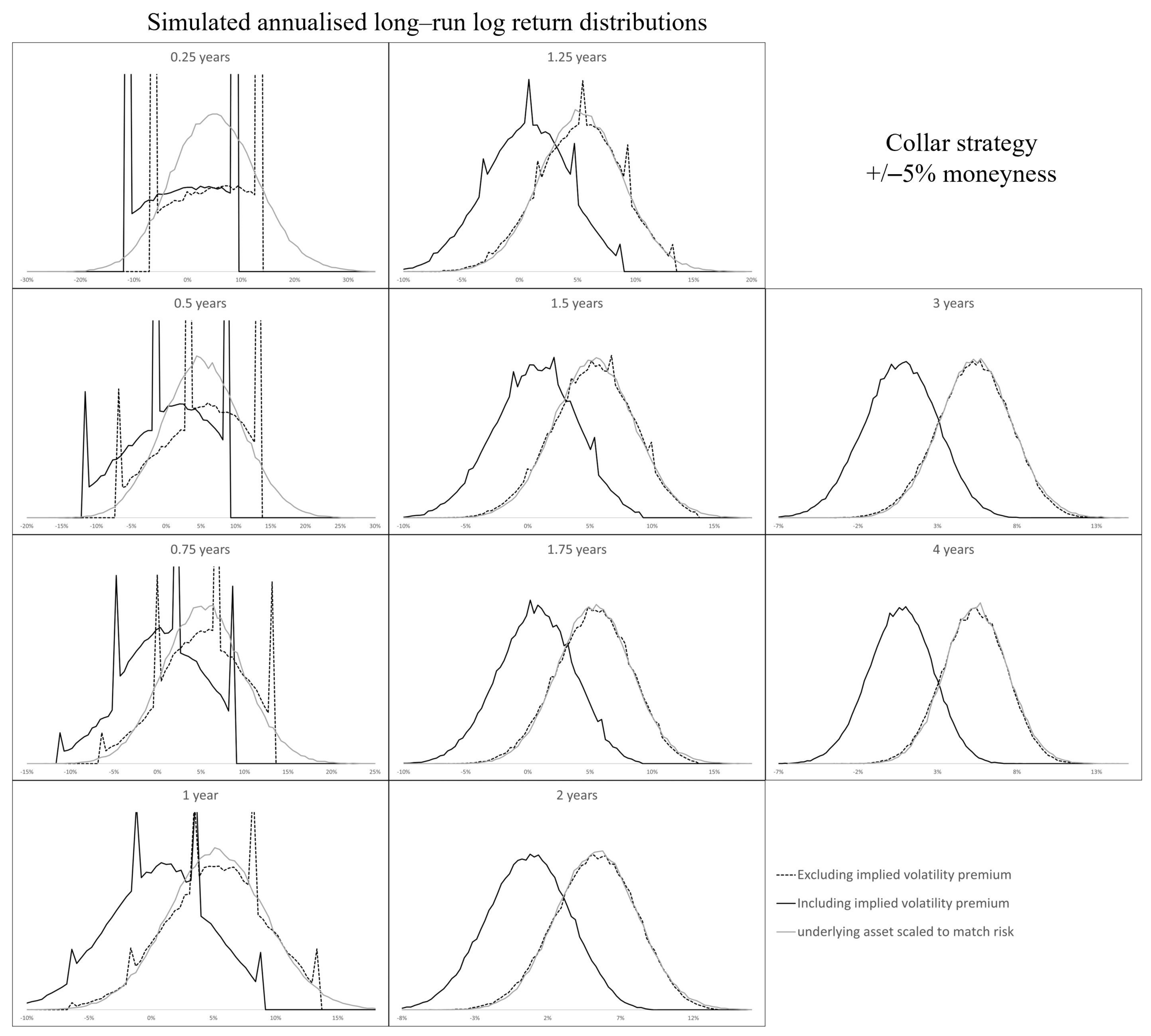
Property A20 
(Long-run option-adjusted portfolio return distribution). If r A ( 1 ) , , r A ( m ) are independent and identically distributed, then the annualised long-run log return of an invariant option-adjusted portfolio tends to a normal distribution as the number of single-periods constituting that long-run tends to infinity.
Proof. 
The long-run log return of the option-adjusted portfolio is defined as
log ( 1 + r O ( 1 ) ) + + log ( 1 + r O ( m ) ) m
The two previous properties have shown that if r A ( 1 ) , , r A ( m ) are independent and identically distributed, and the option-adjusted portfolio is invariant, then r O ( 1 ) , , r O ( m ) are independent and identically distributed. The Existence of log moments of a value function property says that E [ log ( 1 + r O ) ] and V [ log ( 1 + r O ) ] exist (we have omitted the indexing as the expectation and variance will be the same for i = 1 , , m ). Therefore, by the central limit theorem [34], in the limit as m , the long-run log return is normally distributed with mean E [ log ( 1 + r O ) ] and variance V [ log ( 1 + r O ) ] / m . □

References

  1. Hull, J. Options, Futures, and Other Derivative Securities, 2nd ed.; Prentice-Hall International, Inc.: London, UK, 1993. [Google Scholar]
  2. Bodie, Z.; Kane, A.; Marcus, A. Investments, 3rd ed.; Irwin: Chicago, IL, USA, 1996. [Google Scholar]
  3. Borowski, K. Testing 65 equity indexes for normal distribution of return. J. Econ. Manag. 2018, 34, 5–38. [Google Scholar] [CrossRef]
  4. Bookstaber, R.; Clarke, R. Option portfolio strategies: Measurement and evaluation. J. Bus. 1984, 57, 469–492. [Google Scholar] [CrossRef]
  5. Agrrawal, P. Using index ETFs for multi-asset-class investing: Shifting up the efficient frontier. J. Index Invest. 2013, 4, 83–94. [Google Scholar] [CrossRef]
  6. Evnine, J.; Rudd, A. Option portfolio risk analysis. J. Portf. Manag. 1984, 10, 23–27. [Google Scholar] [CrossRef]
  7. Sears, R.; Trennepohl, G. Measuring portfolio risk in options. J. Financ. Quant. Anal. 1982, 17, 391–409. [Google Scholar] [CrossRef]
  8. Figelman, I. Expected return and risk of covered call strategies. J. Portf. Manag. 2008, 34, 81–97. [Google Scholar] [CrossRef]
  9. Goetzmann, W.; Ingersoll, J.; Spiegel, M.; Welch, I. Sharpening Sharpe Ratios; NBER Working Paper Series; Working Paper 9116; NBER: Cambridge, MA, USA, 2002. [Google Scholar]
  10. Israelov, R.; Klein, M. Risk and return of equity index collar strategies. J. Altern. Invest. 2016, 19, 41–54. [Google Scholar] [CrossRef]
  11. Slivka, R. Risk and return for option investment strategies. Financ. Anal. J. 1980, 36, 67–73. [Google Scholar] [CrossRef]
  12. Merton, R.; Scholes, M.; Gladstein, M. The returns and risks of alternative call option portfolio investment strategies. J. Bus. 1978, 36, 67–73. [Google Scholar] [CrossRef]
  13. Merton, R.; Scholes, M.; Gladstein, M. The returns and risks of alternative put option portfolio investment strategies. J. Bus. 1982, 55, 1–55. [Google Scholar] [CrossRef]
  14. Bollen, N. Measuring the Benefits of Option Strategies for Portfolio Management; Research Report for Catalyst Institute; University of Utah: Salt Lake City, UT, USA, 1999. [Google Scholar]
  15. Bookstaber, R.; Clarke, R. Problems in evaluating the performance of portfolio with options. Financ. Anal. J. 1985, 41, 48–62. [Google Scholar] [CrossRef]
  16. Bookstaber, R.; Clarke, R. An algorithm to calculate the return distribution of portfolios with option positions. Manag. Sci. 1983, 29, 419–429. [Google Scholar] [CrossRef]
  17. Bookstaber, R.; Clarke, R. Options can alter portfolio return. J. Portf. Manag. 1981, 7, 63–70. [Google Scholar] [CrossRef]
  18. Cochrane, J. Asset Pricing; Princeton University Press: Princeton, NJ, USA, 2001. [Google Scholar]
  19. Capstone Investment Advisors, LLC. An Overview of Options Strategies; Capstone Investor Relations, Capstone LLC: New York, NY, USA, 2016. [Google Scholar]
  20. Collar. Available online: https://www.fidelity.com/learning-center/investment-products/options/options-strategy-guide/collar (accessed on 30 March 2022).
  21. Capital Market Assumptions. Available online: https://www.blackrock.com/institutions/en-gb/insights/charts/capital-marketassumptions (accessed on 30 March 2022).
  22. Long Term Capital Market Assumptions. Available online: https://am.jpmorgan.com/content/dam/jpm-am-aem/global/en/insights/portfolio-insights/ltcma/ltcma-full-report.pdf (accessed on 30 March 2022).
  23. Long Term Capital Market Assumptions. Available online: https://institutional.fidelity.com/app/literature/white-paper/9904178/capital-market-assumptions-a-comprehensive-global-approach-for-the-next-20-years.html (accessed on 30 March 2022).
  24. Fama, E. The behaviour of stock-market prices. J. Bus. 1965, 38, 34–105. [Google Scholar] [CrossRef]
  25. Tobin, J. Liquidity preference as behaviour towards risk. Rev. Econ. Stud. 1958, XXV, 65–86. [Google Scholar] [CrossRef]
  26. Blattberg, R.; Gonedes, N. A comparison of the stable and student distributions as statistical models for stock prices. J. Bus. 1974, 47, 244–280. [Google Scholar] [CrossRef]
  27. Fama, E. Efficient capital markets: A review of theory and empirical work. J. Financ. 1970, 25, 383–417. [Google Scholar] [CrossRef]
  28. Carhart, M. On persistence in mutual fund performance. J. Financ. 1970, 52, 57–82. [Google Scholar] [CrossRef]
  29. Engle, R. GARCH 101: The use of ARCH/GARCH models in applied econometrics. J. Econ. Perspect. 2001, 15, 157–168. [Google Scholar] [CrossRef] [Green Version]
  30. Ingersoll, J. Theory of Financial Decision Making; Rowman and Littlefield Publishers, Inc.: Lanham, MD, USA, 1987. [Google Scholar]
  31. Cox, J.; Rubenstein, M. Options Markets; Prentice-Hall: Hoboken, NJ, USA, 1985. [Google Scholar]
  32. Browder, A. Mathematical Analysis: An Introduction; Springer: New York, NY, USA, 1996. [Google Scholar]
  33. Ross, S. Options and efficiency. Q. J. Econ. 1976, 90, 75–89. [Google Scholar] [CrossRef]
  34. Feller, W. An Introduction to Probability Theory and Its Applications; John Wiley and Sons, Inc.: Hoboken, NJ, USA, 1968. [Google Scholar]
Figure 1. The payoff profiles of call and put options.
Mathematics 10 01563 g001
Figure 2. The payoff profiles of underlying asset overlaid with: (a) a call overwriting strategy in the first panel; (b) a put protection strategy in the second panel; and (c) a collar strategy in the third panel.
Mathematics 10 01563 g002
Figure 3. The implied volatilities on options on the S&P 500 expiring on 31 March 2022, using closing prices of 3 December 2021, quoted by CBOE. The typical volatility skew is clearly present where implied volatility increases as the strike price decreases.
Mathematics 10 01563 g003
Figure 4. The risk premium for an underlying asset with an overlaid call overwriting strategy for a range of strike prices. The dotted line assumes the implied volatility is equal to the underlying asset volatility. The solid line includes the implied volatility premium in the price of the options.
Mathematics 10 01563 g004
Figure 5. The risk of the return of an underlying asset with an overlaid call overwriting strategy for a range of strike prices.
Mathematics 10 01563 g005
Figure 6. The Sharpe ratio for an underlying asset with an overlaid call overwriting strategy for a range of strike prices. The dotted line assumes the implied volatility is equal to the underlying asset volatility. The solid line includes the implied volatility premium in the price of the options.
Mathematics 10 01563 g006
Figure 7. The price sensitivity (beta) of an underlying asset with an overlaid call overwriting strategy for a range of strike prices in relation to price change of the underlying asset.
Mathematics 10 01563 g007
Figure 8. The expected amount of capital appreciation of a portfolio consisting of an underlying asset and a call overwriting strategy for a range of strike prices, assuming the income from the sale of the call option is distributed to the investor. The expected appreciation is negative if the strike price is less than about 4% out-of-the-money. In this case, the investment will eventually become zero valued.
Mathematics 10 01563 g008
Figure 9. A simulation of the value of an underlying asset overlaid with a call overwriting strategy for 3 strike prices: 5% out-of-the-money, at-the-money, and 5% in-the-money.
Mathematics 10 01563 g009
Figure 10. The risk premium for an underlying asset with an overlaid put protection strategy for a range of strike prices. The dotted line assumes the implied volatility is equal to the underlying asset volatility. The solid line includes the implied volatility premium in the price of the options.
Mathematics 10 01563 g010
Figure 11. The risk of the return of an underlying asset with an overlaid put protection strategy for a range of strike prices.
Mathematics 10 01563 g011
Figure 12. The Sharpe ratio for an underlying asset with an overlaid put protection strategy for a range of strike prices. The dotted line assumes the implied volatility is equal to the underlying asset volatility. The solid line includes the implied volatility premium in the price of the options.
Mathematics 10 01563 g012
Figure 13. The price sensitivity (beta) of an underlying asset with an overlaid put protection strategy for a range of strike prices in relation to price change of the underlying asset.
Mathematics 10 01563 g013
Figure 14. The strike price of a call such that a collar has zero initial cost for a range of put strike prices. The dotted line assumes the implied volatility is equal to the underlying asset volatility. The solid line uses includes the implied volatility premium in the price of the options. The put is more expensive when incorporating the volatility skew, so more capital appreciation must be sacrificed, resulting in a lower call strike price.
Mathematics 10 01563 g014
Figure 15. The risk premium for an underlying asset with an overlaid symmetric collar strategy for a range of strike prices. The dotted line assumes the implied volatility is equal to the underlying asset volatility. The solid line includes the implied volatility premium in the price of the options.
Mathematics 10 01563 g015
Figure 16. The risk of the return of an underlying asset with an overlaid symmetric collar strategy for a range of strike prices.
Mathematics 10 01563 g016
Figure 17. The Sharpe ratio for an underlying asset with an overlaid symmetric collar strategy for a range of strike prices. The dotted line assumes the implied volatility is equal to the underlying asset volatility. The solid line includes the implied volatility premium in the price of the options.
Mathematics 10 01563 g017
Figure 18. The price sensitivity (beta) of an underlying asset with an overlaid symmetric collar strategy for a range of strike prices in relation to price change of the underlying asset.
Mathematics 10 01563 g018
Figure 19. Simulations of the long-run returns of an underlying asset overlaid with a quarterly at-the-money call overwriting strategy over investment horizons of 1 4 year, 1 2 year, 3 4 year, 1 year, 1 1 4 years, 1 1 2 years, 1 3 4 years, 2 years, 3 years, and 4 years. The dotted line assumes the implied volatility is equal to the underlying asset volatility. The solid line includes the implied volatility premium in the price of the options. The gray line shows the long-run returns of a portfolio consisting of the risk-free asset and the underlying asset weighted to have the same risk as the option strategy.
Mathematics 10 01563 g019
Figure 20. Simulations of the long-run returns of an underlying asset overlaid with a quarterly 5% out-of-the-money call overwriting strategy over investment horizons of 1 4 year, 1 2 year, 3 4 year, 1 year, 1 1 4 years, 1 1 2 years, 1 3 4 years, 2 years, 3 years, and 4 years. The dotted line assumes the implied volatility is equal to the underlying asset volatility. The solid line includes the implied volatility premium in the price of the options. The gray line shows the long-run returns of a portfolio consisting of the risk-free asset and the underlying asset weighted to have the same risk as the option strategy.
Mathematics 10 01563 g020
Figure 21. Simulations of the long-run returns of an underlying asset overlaid with a quarterly at-the-money put protection strategy over investment horizons of 1 4 year, 1 2 year, 3 4 year, 1 year, 1 1 4 years, 1 1 2 years, 1 3 4 years, 2 years, 3 years, and 4 years. The dotted line assumes the implied volatility is equal to the underlying asset volatility. The solid line includes the implied volatility premium in the price of the options. The gray line shows the long-run returns of a portfolio consisting of the risk-free asset and the underlying asset weighted to have the same risk as the option strategy.
Mathematics 10 01563 g021
Figure 22. Simulations of the long-run returns of an underlying asset overlaid with a quarterly 5% out-of-the-money call overwriting strategy over investment horizons of 1 4 year, 1 2 year, 3 4 year, 1 year, 1 1 4 years, 1 1 2 years, 1 3 4 years, 2 years, 3 years, and 4 years.. The dotted line assumes the implied volatility is equal to the underlying asset volatility. The solid line includes the implied volatility premium in the price of the options. The gray line shows the long-run returns of a portfolio consisting of the risk-free asset and the underlying asset weighted to have the same risk as the option strategy.
Mathematics 10 01563 g022
Figure 23. Simulations of the long-run returns of an underlying asset overlaid with a quarterly ±5% moneyness symmetric collar strategy over investment horizons of 1 4 year, 1 2 year, 3 4 year, 1 year, 1 1 4 years, 1 1 2 years, 1 3 4 years, 2 years, 3 years, and 4 years. The dotted line assumes the implied volatility is equal to the underlying asset volatility. The solid line uses includes the implied volatility premium in the price of the options. The gray line shows the long-run returns of a portfolio consisting of the risk-free asset and the underlying asset weighted to have the same risk as the option strategy.
Mathematics 10 01563 g023
Figure 24. Simulations of the long-run returns of an underlying asset overlaid with a quarterly ±10% moneyness symmetric collar strategy over investment horizons of 1 4 year, 1 2 year, 3 4 year, 1 year, 1 1 4 years, 1 1 2 years, 1 3 4 years, 2 years, 3 years, and 4 years. The dotted line assumes the implied volatility is equal to the underlying asset volatility. The solid line includes the implied volatility premium in the price of the options. The gray line shows the long-run returns of a portfolio consisting of the risk-free asset and the underlying asset weighted to have the same risk as the option strategy.
Mathematics 10 01563 g024
Table 1. Parameters defining three popular option-adjusted portfolios.
Strategy x i b i a i
Call overwrite x 1 (the price beyond which all upside is sacrificed) b 0 = 1 a 0 = 0
( n = 1 ) b 1 = 0 a 1 = x 1
Put protection x 1 (the price below which downside is protected) b 0 = 0 a 0 = 0
( n = 1 ) b 1 = 1 a 1 = 0
Collar x 1 (the price beyond which all upside is sacrificed) b 0 = 0 a 0 = 0
( n = 2 ) x 2 (the price below which downside is protected) b 1 = 1 a 1 = 0
b 2 = 0 a 2 = x 2 x 1
Publisher’s Note: MDPI stays neutral with regard to jurisdictional claims in published maps and institutional affiliations.

