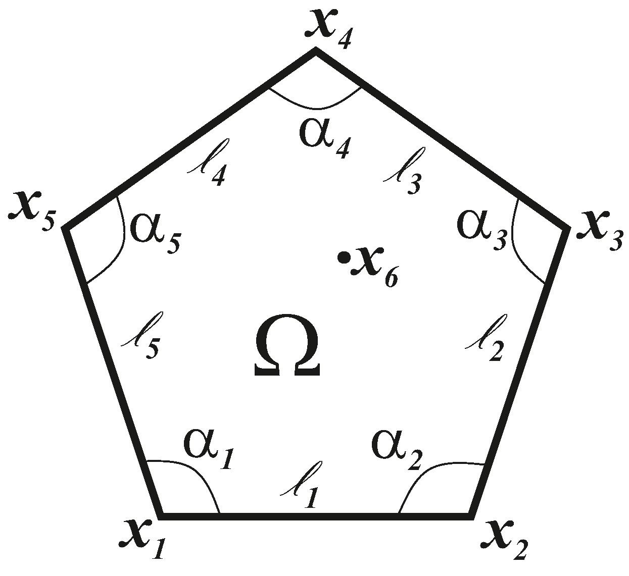
Figure 1.
Example of a 2D configuration made by six landmarks, with the first five lying on the boundary and one, , inside the region .
Figure 1.
Example of a 2D configuration made by six landmarks, with the first five lying on the boundary and one, , inside the region .
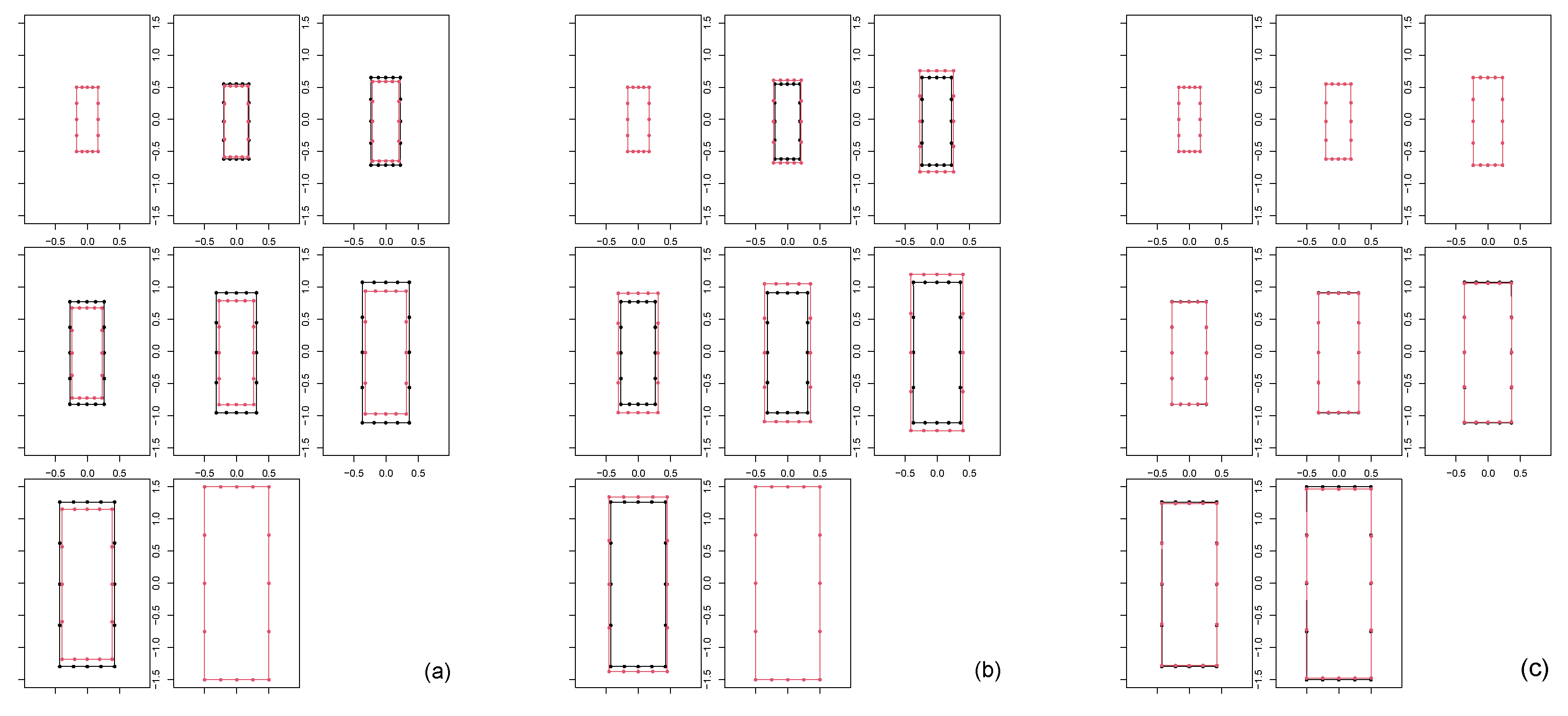
Figure 2.
Affine spherical case results. (a) Left panel: geodesic trajectory shapes (black) plotted against the original parametric shapes (red). (b) Center panel: geodesic trajectory shapes (black) plotted against the shapes found via linear interpolation between the first and last shapes of the parametric dataset (red). (c) Right panel: geodesic trajectory shapes (black) plotted against autoparallel trajectory (red) built via shooting of the first two configurations of the geodesic.
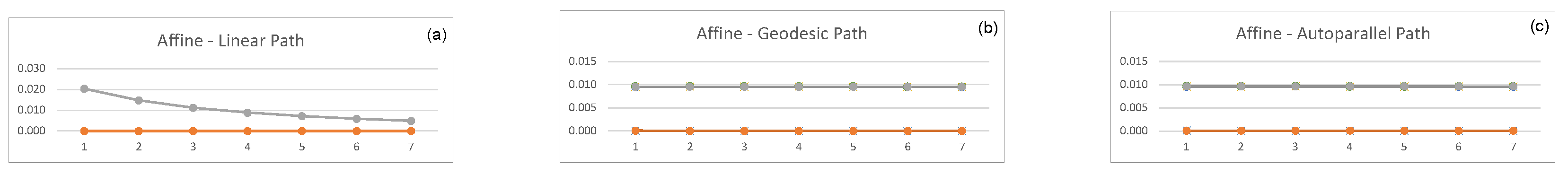
Figure 3.
Trend of the energies for different interpolations: (a) Left: linear interpolation (b) Center: geodesics interpolation. (c) Right: autoparallel interpolation. Blue refers to , red to , grey to .
Figure 3.
Trend of the energies for different interpolations: (a) Left: linear interpolation (b) Center: geodesics interpolation. (c) Right: autoparallel interpolation. Blue refers to , red to , grey to .
Figure 4.
Affine general case results. (a) Left panel: geodesic trajectory shapes (black) plotted against the original parametric shapes (red). (b) Center panel: geodesic trajectory shapes (black) plotted against the shapes found via linear interpolation between the first and last shapes of the parametric dataset (red). (c) Right panel: geodesic trajectory shapes (black) plotted against autoparallel trajectory (red) built via shooting of the first two configurations of the geodesic.
Figure 5.
Trend of the energies for different interpolations: (a) Left: linear interpolation (b) Center: geodesics interpolation. (c) Right: autoparallel interpolation. Blue refers to , red to , grey to .
Figure 5.
Trend of the energies for different interpolations: (a) Left: linear interpolation (b) Center: geodesics interpolation. (c) Right: autoparallel interpolation. Blue refers to , red to , grey to .
Figure 6.
PC1-PC2 scatterplot of the PCA perfomed on the four set of shapes resulting from the general affine case. PC1 explains 97.2% of total variance, while PC2 explains 2.66%. Black refers to the optimized shapes, red to the linearized, green to the original shapes, and cyan to the shooted shapes.
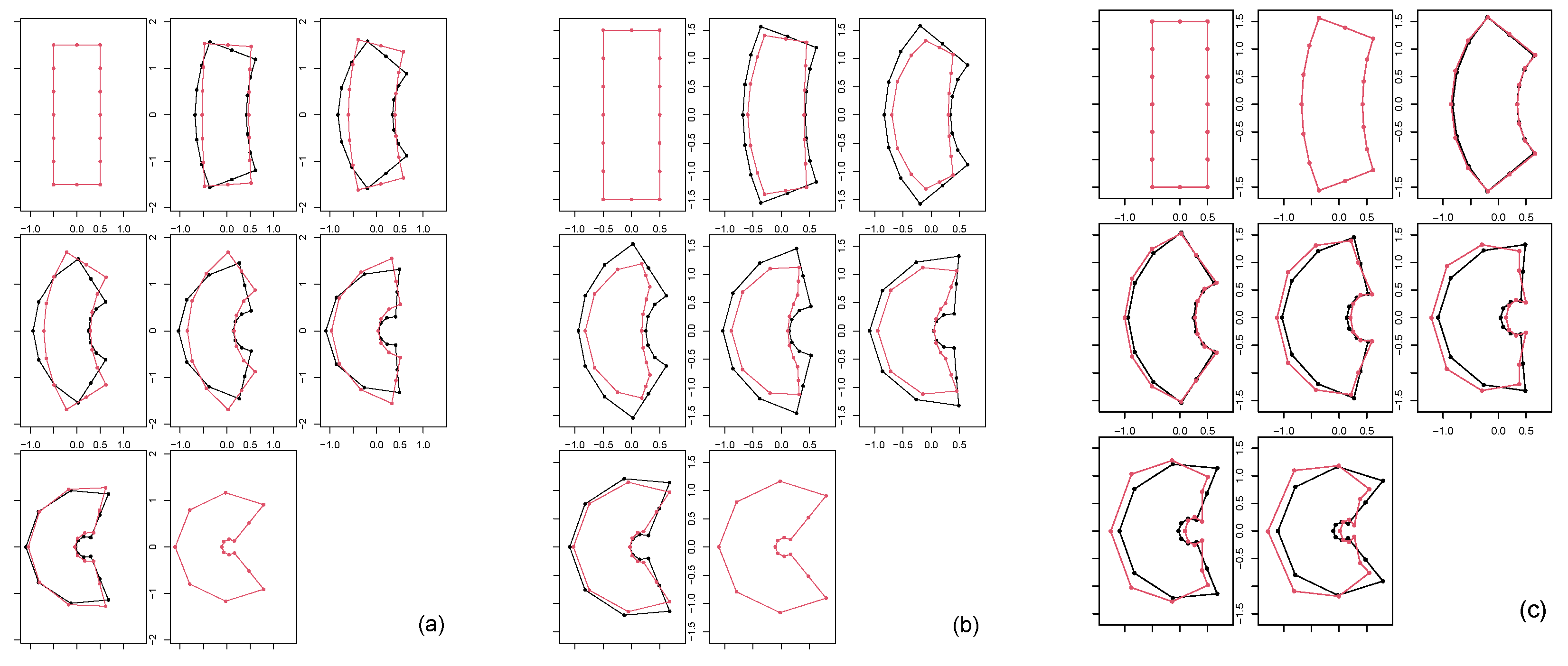
Figure 7.
Non-affine case bending-only results. (a) Left panel: geodesic trajectory shapes (black) plotted against the original parametric shapes (red). (b) Center panel: geodesic trajectory shapes (black) plotted against the shapes found via linear interpolation between the first and last shapes of the parametric dataset (red). (c) Right panel: geodesic trajectory shapes (black) plotted against autoparallel trajectory (red) built via shooting of the first two configurations of the geodesic.
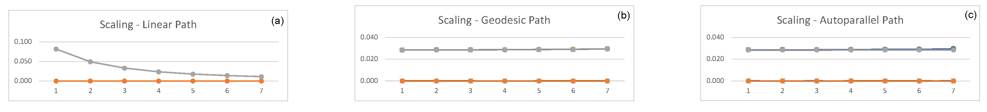
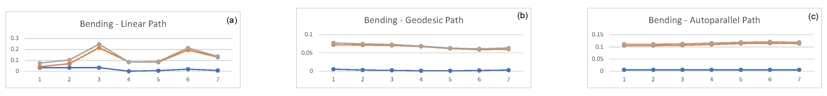
Figure 8.
Trend of the energies for different interpolations: (a) Left: linear interpolation (b) Center: geodesics interpolation. (c) Right: autoparallel interpolation. Blue refers to , red to , grey to .
Figure 8.
Trend of the energies for different interpolations: (a) Left: linear interpolation (b) Center: geodesics interpolation. (c) Right: autoparallel interpolation. Blue refers to , red to , grey to .
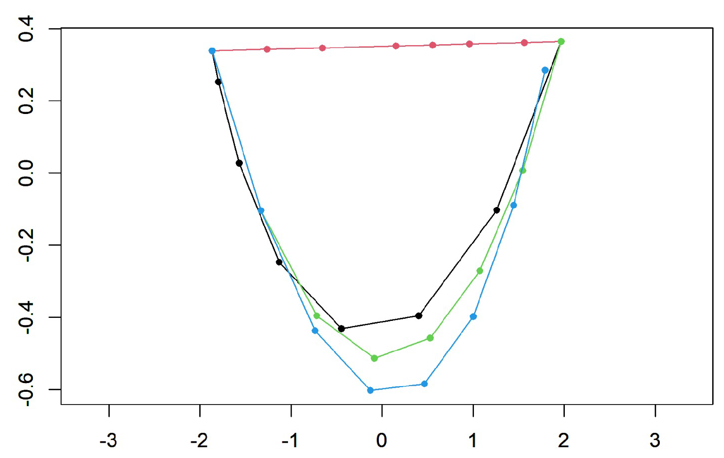
Figure 9.
PC1-PC2 scatterplot of the PCA perfomed on the four set of shapes resulting from the pure bending case. PC1 explains 91.11% of total variance, while PC2 explains 6.50%. Black refers to the optimized shapes, red to the linearized, green to the original shapes and cyan to the shooted shapes.
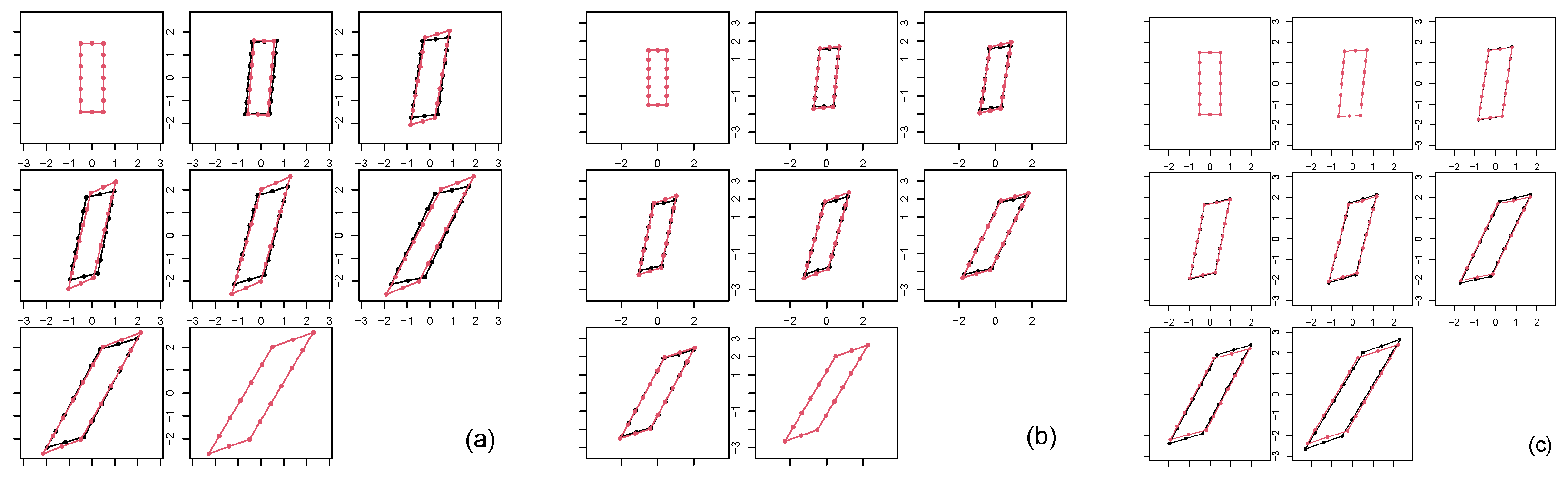
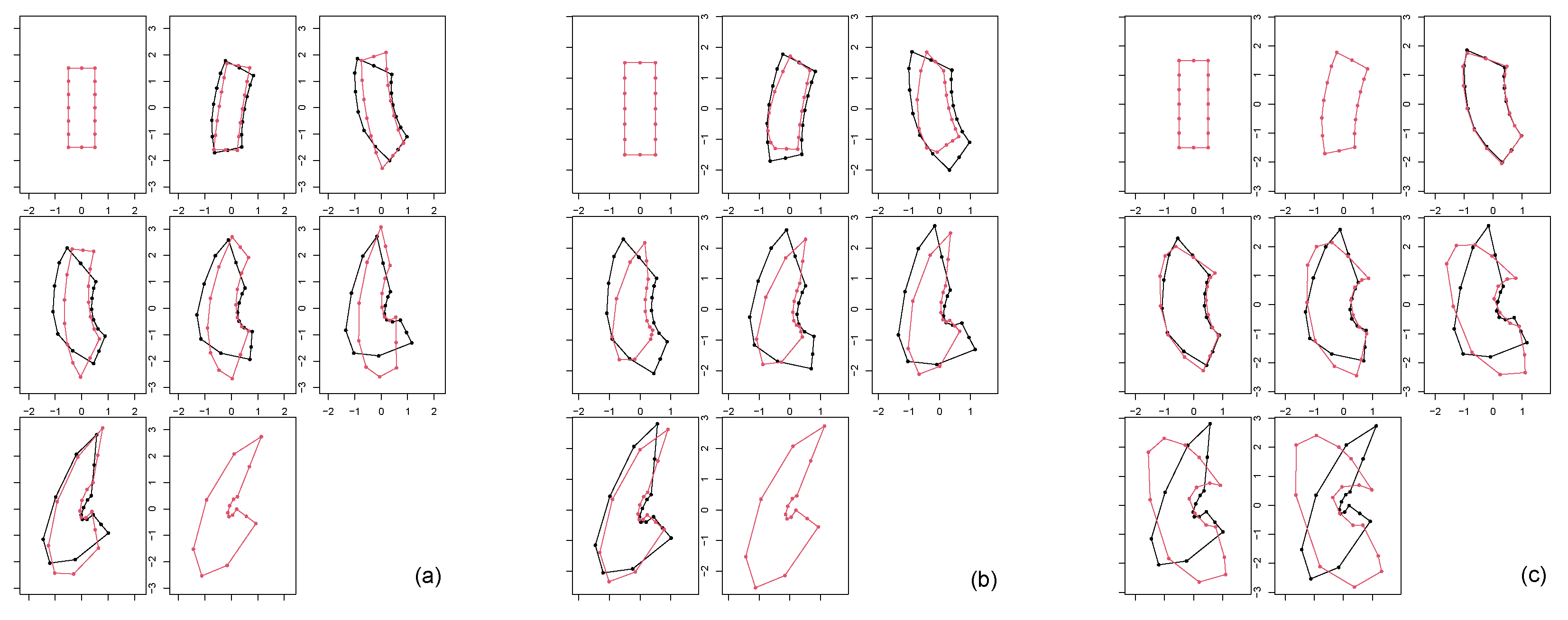
Figure 10.
Non-affine case bending+size results. (a) Left panel: geodesic trajectory shapes (black) plotted against the original parametric shapes (red). (b) Center panel: geodesic trajectory shapes (black) plotted against the shapes found via linear interpolation between the first and last shapes of the parametric dataset (red). (c) Right panel: geodesic trajectory shapes (black) plotted against autoparallel trajectory (red) built via shooting of the first two configurations of the geodesic.
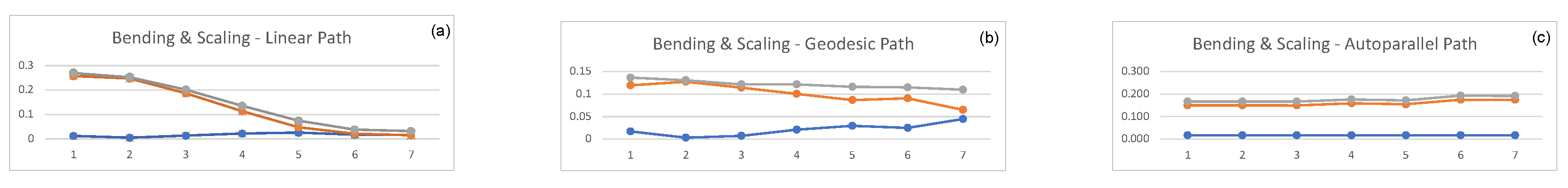
Figure 11.
Trend of the energies for different interpolations: (a) Left: linear interpolation (b) Center: geodesics interpolation. (c) Right: autoparallel interpolation. Blue refers to , red to , grey to .
Figure 11.
Trend of the energies for different interpolations: (a) Left: linear interpolation (b) Center: geodesics interpolation. (c) Right: autoparallel interpolation. Blue refers to , red to , grey to .
Figure 12.
PC1-PC2 scatterplot of the PCA perfomed on the four set of shapes resulting from the bending+size case. PC1 explains 79.36% of total variance, while PC2 explains 17.54%. Black refers to the optimized shapes, red to the linearized, green to the original shapes and cyan to the shooted shapes.
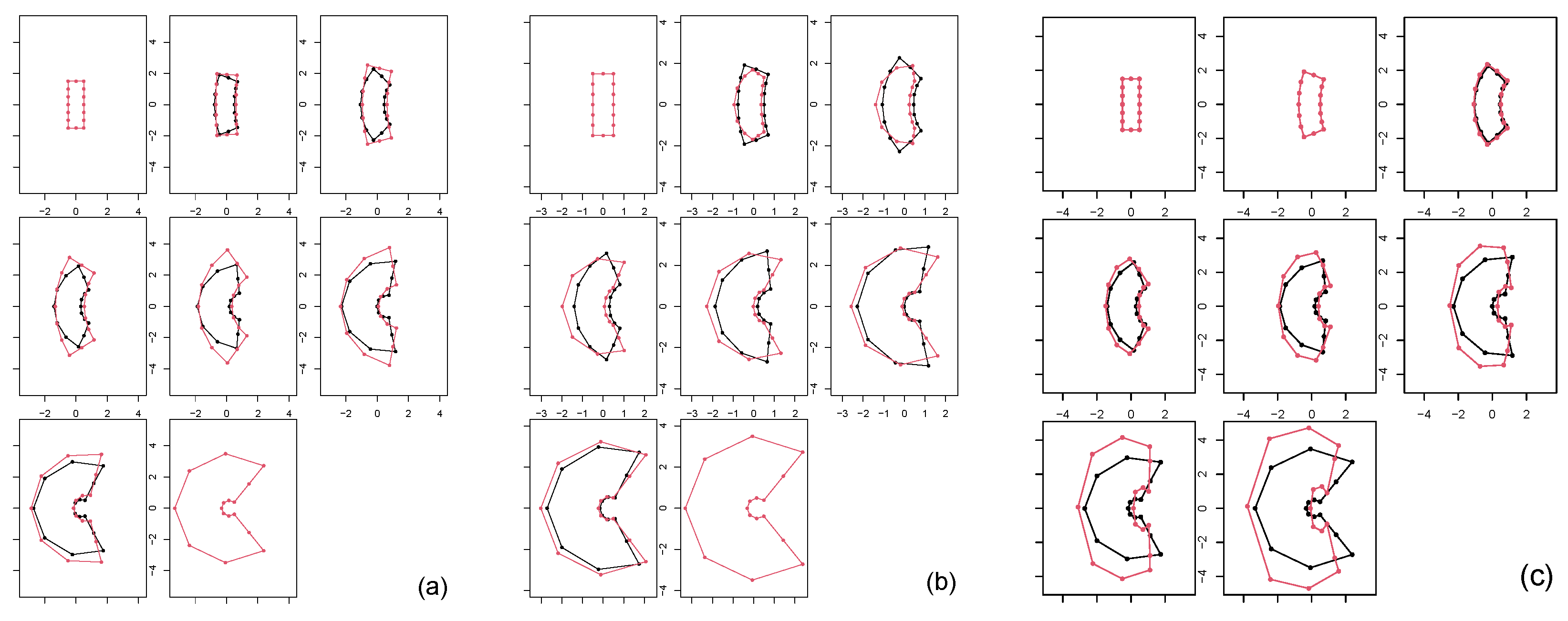
Figure 13.
Non-affine case, bending+general affine component, results. (a) Left panel: geodesic trajectory shapes (black) plotted against the original parametric shapes (red). (b) Center panel: geodesic trajectory shapes (black) plotted against the shapes found via linear interpolation between the first and last shapes of the parametric dataset (red). (c) Right panel: geodesic trajectory shapes (black) plotted against autoparallel trajectory (red) built via shooting of the first two configurations of the geodesic.
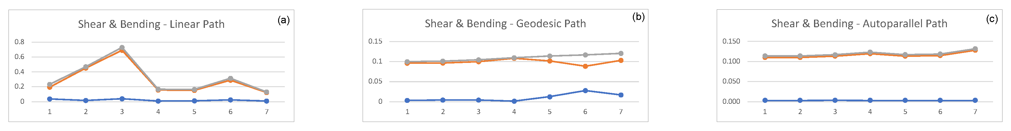
Figure 14.
Trend of the energies for different interpolations: (a) Left: linear interpolation (b) Center: geodesics interpolation. (c) Right: autoparallel interpolation. Blue refers to , red to , grey to .
Figure 14.
Trend of the energies for different interpolations: (a) Left: linear interpolation (b) Center: geodesics interpolation. (c) Right: autoparallel interpolation. Blue refers to , red to , grey to .
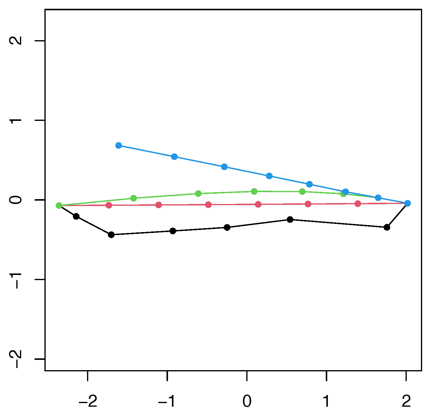
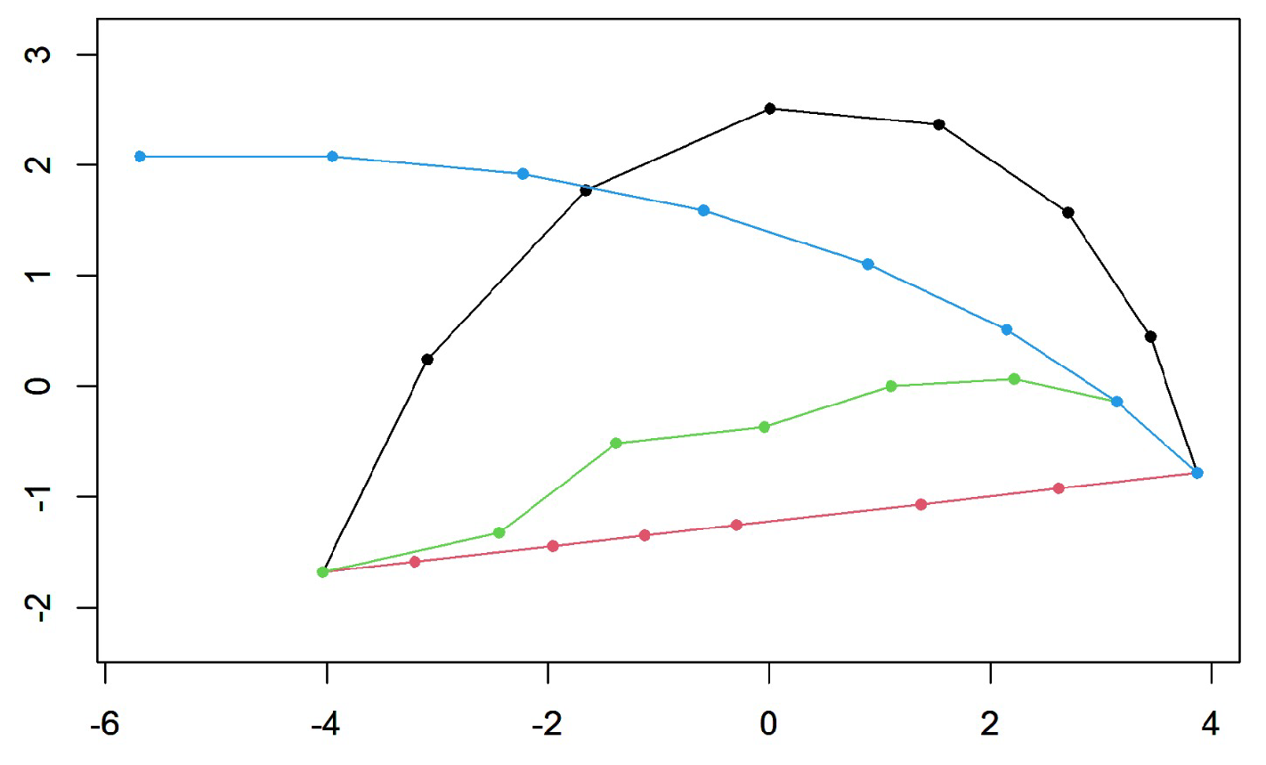
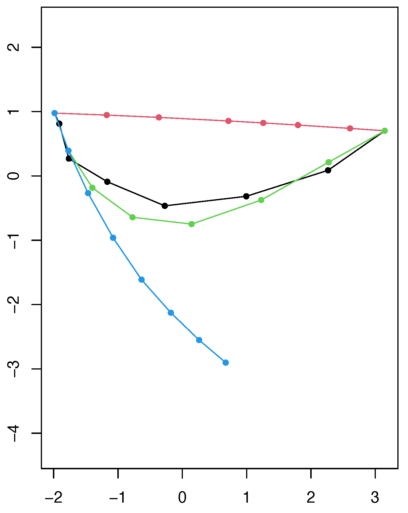
Figure 15.
PC1-PC2 scatterplot of the PCA perfomed on the four set of shapes resulting from the bending+general affine component case. PC1 explains 62.61% of total variance, while PC2 explains 25.48%. Black refers to the optimized shapes, red to the linearized, green to the original shapes and cyan to the shooted shapes.
Table 1.
Values of the energies for the affine spherical case; represents the affine component of the -energy, the non-affine component and the total -energy.
Table 1.
Values of the energies for the affine spherical case; represents the affine component of the -energy, the non-affine component and the total -energy.
| | LINEAR | | | GEODESIC | | | A-PARALLEL | |
|---|
| | | | | | | | |
| 0.082 | 0.000 | 0.082 | 0.029 | 0.000 | 0.029 | 0.029 | 0.000 | 0.029 |
| 0.049 | 0.000 | 0.049 | 0.029 | 0.000 | 0.029 | 0.029 | 0.000 | 0.029 |
| 0.033 | 0.000 | 0.033 | 0.029 | 0.000 | 0.029 | 0.029 | 0.000 | 0.029 |
| 0.024 | 0.000 | 0.024 | 0.029 | 0.000 | 0.029 | 0.029 | 0.000 | 0.029 |
| 0.018 | 0.000 | 0.018 | 0.029 | 0.000 | 0.029 | 0.029 | 0.000 | 0.029 |
| 0.014 | 0.000 | 0.014 | 0.029 | 0.000 | 0.029 | 0.029 | 0.000 | 0.029 |
| 0.011 | 0.000 | 0.011 | 0.030 | 0.000 | 0.030 | 0.029 | 0.000 | 0.029 |
Table 2.
Values of the energies for the affine general case; represents the affine component of the -energy, the non-affine component, and the total -energy.
Table 2.
Values of the energies for the affine general case; represents the affine component of the -energy, the non-affine component, and the total -energy.
| | LINEAR | | | GEODESIC | | | A-PARALLEL | |
|---|
| | | | | | | | |
| 0.020 | 0.000 | 0.020 | 0.010 | 0.000 | 0.010 | 0.010 | 0.000 | 0.010 |
| 0.015 | 0.000 | 0.015 | 0.010 | 0.000 | 0.010 | 0.010 | 0.000 | 0.010 |
| 0.011 | 0.000 | 0.011 | 0.010 | 0.000 | 0.010 | 0.010 | 0.000 | 0.010 |
| 0.009 | 0.000 | 0.009 | 0.010 | 0.000 | 0.010 | 0.010 | 0.000 | 0.010 |
| 0.007 | 0.000 | 0.007 | 0.010 | 0.000 | 0.010 | 0.010 | 0.000 | 0.010 |
| 0.006 | 0.000 | 0.006 | 0.010 | 0.000 | 0.010 | 0.010 | 0.000 | 0.010 |
| 0.005 | 0.000 | 0.005 | 0.010 | 0.000 | 0.010 | 0.010 | 0.000 | 0.010 |
Table 3.
Values of the energies for the non-affine case of bending: represents the affine component of the -energy, the non-affine component, and the total -energy.
Table 3.
Values of the energies for the non-affine case of bending: represents the affine component of the -energy, the non-affine component, and the total -energy.
| | LINEAR | | | GEODESIC | | | A-PARALLEL | |
|---|
| | | | | | | | |
| 0.033 | 0.042 | 0.075 | 0.005 | 0.072 | 0.077 | 0.005 | 0.106 | 0.111 |
| 0.034 | 0.070 | 0.104 | 0.003 | 0.072 | 0.075 | 0.005 | 0.106 | 0.111 |
| 0.033 | 0.215 | 0.248 | 0.002 | 0.071 | 0.073 | 0.005 | 0.107 | 0.112 |
| 0.001 | 0.084 | 0.085 | 0.001 | 0.068 | 0.069 | 0.005 | 0.110 | 0.115 |
| 0.006 | 0.084 | 0.090 | 0.001 | 0.062 | 0.063 | 0.005 | 0.114 | 0.119 |
| 0.020 | 0.195 | 0.214 | 0.002 | 0.059 | 0.061 | 0.005 | 0.115 | 0.120 |
| 0.008 | 0.129 | 0.137 | 0.003 | 0.061 | 0.064 | 0.005 | 0.114 | 0.119 |
Table 4.
Values of the energies for the non-affine case of bending and scaling; represents the affine component of the -energy, the non-affine component, and the total -energy.
Table 4.
Values of the energies for the non-affine case of bending and scaling; represents the affine component of the -energy, the non-affine component, and the total -energy.
| | LINEAR | | | GEODESIC | | | A-PARALLEL | |
|---|
| | | | | | | | |
| 0.060 | 0.37 | 0.431 | 0.017 | 0.120 | 0.137 | 0.017 | 0.150 | 0.167 |
| 0.003 | 0.41 | 0.412 | 0.003 | 0.128 | 0.131 | 0.017 | 0.150 | 0.167 |
| 0.147 | 0.42 | 0.571 | 0.007 | 0.115 | 0.122 | 0.017 | 0.150 | 0.168 |
| 0.028 | 0.04 | 0.073 | 0.021 | 0.101 | 0.122 | 0.017 | 0.159 | 0.177 |
| 0.021 | 0.03 | 0.056 | 0.029 | 0.087 | 0.116 | 0.017 | 0.155 | 0.172 |
| 0.036 | 0.07 | 0.104 | 0.025 | 0.091 | 0.115 | 0.017 | 0.176 | 0.193 |
| 0.012 | 0.03 | 0.040 | 0.044 | 0.065 | 0.110 | 0.017 | 0.175 | 0.193 |
Table 5.
Values of the energies for the non-affine case of bending and general affine deformation; represents the affine component of the -energy, the non-affine component, and the total -energy.
Table 5.
Values of the energies for the non-affine case of bending and general affine deformation; represents the affine component of the -energy, the non-affine component, and the total -energy.
| | LINEAR | | | GEODESIC | | | A-PARALLEL | |
|---|
| | | | | | | | |
| 0.037 | 0.196 | 0.233 | 0.004 | 0.096 | 0.100 | 0.004 | 0.110 | 0.114 |
| 0.017 | 0.453 | 0.470 | 0.005 | 0.097 | 0.101 | 0.004 | 0.110 | 0.114 |
| 0.039 | 0.689 | 0.729 | 0.005 | 0.100 | 0.104 | 0.004 | 0.113 | 0.117 |
| 0.010 | 0.158 | 0.168 | 0.001 | 0.108 | 0.110 | 0.004 | 0.120 | 0.123 |
| 0.012 | 0.152 | 0.164 | 0.013 | 0.101 | 0.114 | 0.004 | 0.114 | 0.117 |
| 0.025 | 0.289 | 0.315 | 0.028 | 0.089 | 0.117 | 0.004 | 0.115 | 0.119 |
| 0.009 | 0.124 | 0.132 | 0.017 | 0.103 | 0.120 | 0.004 | 0.128 | 0.132 |


 ,
, 


