A Deep Neural Network Approach to Solving for Seal’s Type Partial Integro-Differential Equation

Abstract

In this paper, we study the problem of solving Seal’s type partial integro-differential equations (PIDEs) for the classical compound Poisson risk model. A data-driven deep neural network (DNN) method is proposed to calculate finite-time survival probability, and an alternative scheme is also investigated when claim payments are exponentially distributed. The DNN method is then extended to the numerical solution of generalized PIDEs. Numerical approximation results under different claim distributions are given, which show that the proposed scheme can obtain accurate results under different claim distributions.

1. Introduction

Classical ruin theory is motivated by quantifying the insolvency of an insurance company and plays an important role in risk management. It uses a model to simplify an insurance company’s operation and examines the evolution of its surplus level over time. In the classical risk model , it is assumed that the insurer starts with some non-negative amount of capital, and then the surplus level changes by receiving premiums from policyholders and paying out claim payments to beneficiaries. Ruin theory has attracted many researchers’ attention, and many scholars have studied the possibility of bankruptcy that an insurance company faces, which is expressed as ruin probability. It can also be seen that the ruin probability and the survival probability are important reference benchmarks for insurance companies that seek to control risks and manage their capital. Hence, it is of practical significance and value to study the ruin probability and survival probability of insurance companies.

The PIDEs we discuss in this paper are based on the compound Poisson process. Based on the characteristics of this process, it can be widely used in the study of ruin-related variables in the fields of insurance actuarial calculations, financial asset pricing, and other problems. In addition, given that the fractional evolution equation is an important example of a PIDE, it contains the integral definition of the fractional Laplacian operator, which is driven by the $\alpha$-stable Lévy process. The fractional Laplacian operator appears in many applications [1,2,3], including turbulent fluids, contaminant transport in fractured rocks, chaotic dynamics, and so on.

In ruin theory, many mathematical models are used to describe the surplus process of an insurance company, such as the classical compound Poisson risk model, the Sparre Andersen risk model, the Markov-modulated risk model, etc. Using different risk models, the research of infinite-time ruin problems has achieved fruitful results. There have been many works devoted to the probability density function of the ruin time and the joint probability density, including the ruin time (see, e.g., [4,5,6,7] and the references therein). Constantinescu et al. (2018) obtained three equivalent expressions for ruin probabilities in a classical risk model with gamma-distributed claims by means of (inverse) Laplace transforms, where two of these expressions involved Mittag-Leffler functions and the third involved the moments of the claim distributions [8].

In contrast to the ultimate ruin probability, the finite-time ruin probability plays a more important role in practice because it can provide insurers with more effective information to aid in controlling their risk. The authors of [9] presented an explicit formula for the Laplace transform in time; it defined the finite-time ruin probabilities of a classical Levy model with phase-type claims. Willmot (2015) demonstrated that, by using the Laplace transform and the Lagrange implicit function theorem, a solution for a generalized PIDE can be obtained [10,11]. Furthermore, many scholars have studied approximate methods for finite-time ruin probability and survival probability under various risk models [12,13,14,15,16,17]. Cheung and Zhang (2021) [18] developed an approximation of ruin probability by using Laguerre series expansion as a function of the initial surplus level, where no specific distributional assumption regarding the claim amounts is required. Moreover, nonparametric estimation methods are also used in the study of ruin-related variables (see [19,20,21]).

In contrast to traditional numerical approximation methods, a neural network offers great advantages in the approximation of complex functions due to its nonlinear structure. Therefore, in recent years, many scholars have conducted in-depth research using neural networks to solve mathematical physical equations. For example, the physical mechanisms of neural networks are used to solve nonlinear PDEs and nonlinear backward differential equations [22,23,24,25,26]. In addition, some scholars have applied neural networks to the problem of option pricing [27,28,29,30]. In addition, deep learning methods for non-local models on bounded regions have been discussed in some recent work (see [31,32,33]).

In this paper, we first propose a new high-precision method based on DNNs to determine finite-time survival probability with unspecified claim distribution and then extend it to solve more general PIDEs. This paper is organized as follows: the classical risk model and renewal PIDEs are described in Section 2. In Section 3, we describe the DNN method for calculating finite-time survival probability in the classical risk model. In Section 4, we extend the approach to solve for a general case of PIDEs and to derive an alternative method for use when individual claim size is exponentially distributed. Finally, some numerical examples are given in Section 5 to illustrate the efficiency and accuracy of the proposed method.

2. Preliminaries

The surplus process under the classical compound Poisson risk model is defined as

$$\begin{array}{c}\hfill U(t)=u+ct-{\displaystyle \sum _{i=1}^{N_t}}{X}_i,\end{array}$$

(1)

where $u\ge 0$ is the insurer’s initial capital; c is the rate of premium income per unit time; $\{N_t,t\ge 0\}$ denotes the number of claims up to time t, which is assumed to be a Poisson process with Poisson rate $\lambda$; and $\{X_i,i=1,2,\dots \}$ is a sequence of independent and identically distributed positive random variables that are independent of $\{N_t,t\ge 0\}$. The random variable ${\left\{X_i\right\}}_{i=1}^{\infty }$ represents the amount of the $i_{th}$ claim, which has the distribution function $P(x)=1-\overline{P}(x)=\mathrm{Pr}(X\le x),x\ge 0$ and the density function $p(x)$. The positive loading condition is assumed, whereby $c=(1+\theta )\lambda E(X)$ with $\theta >0$, which ensures that the average income is greater than the average claim so that ruin is not guaranteed. The aggregate claims $S_t={\sum }_{i=1}^{N_t}{X}_i$ have the mass point $\mathrm{Pr}(S_t=0)=e^{-\lambda t}$ at 0, and the density $f(x,t)$ for $x>0$, given by

$$\begin{array}{c}\hfill f(x,t)={\displaystyle \sum _{n=1}^{\infty }}\frac{{(\lambda t)}^n{e}^{-\lambda t}}{n!}{p}^{\ast n}(x),\end{array}$$

(2)

where $p^{\ast n}$ denotes the density function of $Y_n=X_1+X_2+\dots +X_n$. Then $F(x,t)=\mathrm{Pr}(S_t\le x)$ satisfies

$$F(x,t)=e^{-\lambda t}+{\int }_0^{x}f(\xi ,t)d\xi ,\hspace{1em}x\ge 0.$$

In the classical risk model, the time of ruin is defined as $T_u=\inf \{t\ge 0:U(t)\le 0|U(0)=u\}$, with $T_u=\infty$ if $U(t)\ge 0$ for $t\ge 0$. The finite-time ruin probability is defined as $\psi (u,t)=\mathrm{Pr}(T_u<t|U(0)=u)$, and the finite-time survival probability can be denoted as $\varphi (u,t)=1-\psi (u,t)$. It is well known that $\varphi (u,t)$ satisfies the following PIDE,

$$\begin{array}{c}\hfill \frac{\partial }{\partial t}\varphi (u,t)=c\frac{\partial }{\partial u}\varphi (u,t)-\lambda \varphi (u,t)+\lambda {\int }_0^u\varphi (u-x,t)p(x)dx,\end{array}$$

(3)

with $\varphi (u,0)=1$.

3. Deep Neural Network (DNN) Approach

In this section, DNN methodology is introduced and then used to solve Equation (3). The idea of this method is to construct a function ${\varphi }_{\theta }$ using neural networks that satisfies the original PIDE. More intuitively, ${\varphi }_{\theta }$ is an approximation of the analytic solution of Equation (3), and it represents a function that is realized by a neural network with parameters $\theta$. The parameters $\theta$ include weight matrices $W_i$ and bias vectors $b_i$$(i=1,2,\dots ,M)$, where M represents the depth of the neural network structure, that is, the number of hidden layers. DNNs give the best approximation of the original function by minimizing the loss function. Thus, for any u and t, the goal is to make the following equation true:

$$\begin{array}{c}\hfill \frac{\partial }{\partial t}{\varphi }_{\theta }(u,t)=c\frac{\partial }{\partial u}{\varphi }_{\theta }(u,t)-\lambda {\varphi }_{\theta }(u,t)+\lambda {\int }_0^u{\varphi }_{\theta }(u-x,t)p(x)dx.\end{array}$$

(4)

For an initialized neural network with initial parameters $\theta$, since the parameters $\theta$ are randomly given, Equation (4) may not hold for every u and t; if that is the case, it results in a data error $E_{\theta }(u,t)$,

$$\begin{array}{c}\hfill E_{\theta }(u,t):=\frac{\partial }{\partial t}{\varphi }_{\theta }(u,t)+\mathcal{N}[u,t,{\varphi }_{\theta }],\end{array}$$

(5)

where $\mathcal{N}[·]$ is a nonlinear time-dependent differential operator that represents the network function,

$$\mathcal{N}[u,t,{\varphi }_{\theta }]=-c\frac{\partial }{\partial u}{\varphi }_{\theta }(u,t)+\lambda {\varphi }_{\theta }(u,t)-\lambda {\int }_0^u{\varphi }_{\theta }(u-x,t)p(x)dx.$$

The aim is to train the neural network to find an optimal parameter ${\theta }^{\ast }$; hence, the error of all training data points should be minimized under the corresponding ${\varphi }_{{\theta }^{\ast }}$ of a given parameter. Therefore, we introduce the loss function $L_{\theta }(X)$; according to the optimization theory, we know that in the DNN method, the optimal parameter $\theta ={\theta }^{\ast }$ can be obtained by minimizing the loss function $L_{\theta }(X)$,

$$\begin{array}{cc}\hfill & L_{\theta }(X):=L_{\theta }^E(X^E)+L_{\theta }^I(X^I),\hfill \\ \hfill & {\theta }^{\ast }=\arg \min L_{\theta }(X),\hfill \end{array}$$

(6)

where X denotes the collection of the training data. The loss function $L_{\theta }$ consists of two parts: the mean square error of the data points within the region and the mean square error of the data points satisfying the initial condition.

• The mean square error of the data points within the region

  $$L_{\theta }^E(X^E):=\frac{1}{D_E}{\displaystyle \sum _{i=1}^{D_E}}|E_{\theta }(u_i^E,t_i^E){|}^2,$$

  (7)

  in a training data set $X^E:={\left\{(u_i^E,t_i^E)\right\}}_{i=1}^{N_E}\subset [0,\infty )\times (0,\infty )$.
• The mean squared error with respect to the initial condition

  $$L_{\theta }^I(X^I):=\frac{1}{D_I}{\displaystyle \sum _{i=1}^{D_I}}|{\varphi }_{\theta }(u_i^I,t_i^I)-{\varphi }_I(u_i^I){|}^2,$$

  (8)

  in a number of points $X^I:={\left\{(u_i^I,t_i^I)\right\}}_{i=1}^{N_I}\subset [0,\infty )\times \left\{0\right\}$, where ${\varphi }_{\theta }$ is the neural network approximation of the solution $\varphi :[0,\infty )\times [0,\infty )\to \mathbb{R}$. ${\varphi }_I$ denotes the initial value function.

Note that the training data X consists of all data points extracted in time direction t and space direction u. In order to minimize the loss function $L_{\theta }(X)$ to obtain an approximate solution for Equation (3), DNNs require a further differentiation to evaluate the differential operators ${\partial }_t{\varphi }_{\theta }$ and $\mathcal{N}[{\varphi }_{\theta }]$. Thus, $L_{\theta }(X)$ shares the same parameters as the original network ${\varphi }_{\theta }$. Both types of derivatives can be easily determined through automatic differentiation with machine learning libraries, such as TensorFlow or PyTorch.

It is worth noting that the convolution term in neural network training makes the calculation extremely complicated. Therefore, in order to solve this problem, we use the general Simpson’s rule (GSR) to discretize the convolution term on the right side of Equation (4). Letting $g_{\theta }(x,t)={\varphi }_{\theta }(u-x,t)p(x)$, we have the following discrete form,

$$\begin{array}{cc}\hfill {\int }_0^u{\varphi }_{\theta }(u-x,t)p(x)dx\approx & \frac{u}{6N_u}[g_{\theta }(0,t)+4{\displaystyle \sum _{k=1}^{N_u}}{g}_{\theta }((2k-1){\delta }_u,t)\hfill \\ \hfill & +2{\displaystyle \sum _{k=1}^{N_u-1}}{g}_{\theta }(2k{\delta }_u,t)+g_{\theta }(u,t)],\hfill \end{array}$$

(9)

where $N_u=u/2{\delta }_u$ and ${\delta }_u>0$ is a given value. Then, the network function $\mathcal{N}[u,t,{\varphi }_{\theta }]$ can be written as

$$\begin{array}{cc}\hfill \mathcal{N}[u,t,{\varphi }_{\theta }]& \approx -c\frac{\partial }{\partial u}{\varphi }_{\theta }(u,t)+\lambda {\varphi }_{\theta }(u,t)-\lambda \frac{u}{6N_u}[g_{\theta }(0,t)+4{\displaystyle \sum _{k=1}^{N_u}}{g}_{\theta }((2k-1){\delta }_u,t)\hfill \\ \hfill & +2{\displaystyle \sum _{k=1}^{N_u-1}}{g}_{\theta }(2k{\delta }_u,t)+g_{\theta }(u,t)].\hfill \end{array}$$

The neural networks considered in this paper are multilayer feed-forward neural networks; such networks are compositions of the alternating affine linear function $z=X·W+b$ and the nonlinear function $\sigma (·)$, which are called activation functions. The training data set is transformed by the weight matrix and bias matrix at each hidden layer, and then the result is fed back to the next hidden layer through the action of the activation function. The core of the neural network learning method is to approximate the objective function by combining multiple linear and nonlinear functions; as a result

$$\begin{array}{cc}\hfill {\varphi }_{\theta }(X)& =({\sigma }_L({\sigma }_{L-1}(\cdots {\sigma }_1(X·W_1+b_1)\cdots )W_{L-1}+b_{L-1})·W_L+b_L)·W_{out}+b_{out}\hfill \\ \hfill & ={\sigma }_L\circ \cdots \circ {\sigma }_1(X)·W_{out}+b_{out},\hfill \end{array}$$

where $W_i$ and $b_i$$(i=1,2,\dots ,L-1)$ are weight matrices and bias vectors in the $i_{th}$ hidden layer, $W_{out}$ and $b_{out}$ denote the parameters in the output layer, and ${\sigma }_i(·)$ represents the $i_{th}$ layer activation function, which is an element-wise nonlinear function. Generally speaking, the most commonly used activation functions are the following:

• Sigmoid function

  $$s(x)=\frac{1}{1+e^{-ax}}.$$

  The output mapping of the sigmoid function is within the range of $[0,1]$, the function is monotone continuous, and the output range is limited, so it is easy to differentiate. However, it is also easy to saturate, resulting in poor training effectiveness.
• Tanh function

  $$\tanh (x)=\frac{\sinh (x)}{\cosh (x)}=\frac{e^x-e^{-x}}{e^x+e^{-x}}.$$

  The shape of this function is similar to the sigmoid function, except that the tanh function is in the range of [−1,1]; thus, it has the advantage that it is more easily able to handle negative numbers. When the two functions are compared, the tanh function converges faster than the sigmoid function, and the data distribution is more even. However, its drawback is the disappearance of the gradient due to saturation.
• ReLU function

  $$\mathrm{relu}(x)=\max (0,x).$$

  Compared with the previous two activation functions, the ReLU function can converge quickly in the stochastic gradient descent algorithm, and since its gradient is 0 or constant, it can alleviate the problem of gradient disappearance. However, as training goes on, the neurons may die; the weights cannot be renewed, so if this occurs, the gradient passing through those neurons is always 0 from that point onward.

Normally, the training of networks consists of updating the parameter $\theta$ based on gradient optimization during the back propagation of the neural networks. The goal is to find the parameter ${\theta }^{\ast }$ that minimizes the loss function. This procedure requires ${\varphi }_{\theta }$ to differentiate its unknown parameters $W_i$ and $b_i$, that is, to further evaluate the differential operators ${\partial }_t{\varphi }_{\theta }$ and $\mathcal{N}[·]$. The “gradient” plays a crucial role in this process. It implies the direction in which the parameters $\theta$ vary. More precisely, it tells us how to change the parameters $\theta$ to make the loss function change as quickly as possible.

We know that a single hidden layer network can form a deep neural network by increasing the number of hidden layers. In order to facilitate the expression, we take a network with three hidden layers, as shown in Figure 1, as an example. For the training data set $X={\{X_i=(u_i,t_i)\}}_{i=1}^N$, the network output ${\varphi }_{\theta }(X_i)$ can be expressed as

$$\begin{array}{ccc}\hfill {\varphi }_{\theta }(X_i)& =& ({\sigma }_3({\sigma }_2({\sigma }_1(X_i·W_1+b_1)·W_2+b_2)·W_3+b_3)·W_{out}+b_{out}\hfill \\ & =& {\sigma }_3\circ {\sigma }_2\circ {\sigma }_1(X_i)·W_{out}+b_{out}.\hfill \end{array}$$

(10)

Here, we assume that the number of neurons in the hidden layers are $N_1$, $N_2$, and $N_3$. Then, $W_1$, $W_2$, and $W_{out}$ are weight matrices of the following form

$$W_1={\left(\begin{array}{cccc}{w}_{11}^{(1)}& w_{12}^{(1)}& \cdots & w_{1N_1}^{(1)}\\ w_{21}^{(1)}& w_{22}^{(1)}& \cdots & w_{2N_1}^{(1)}\end{array}\right)}_{2\times N_1},W_2={\left(\begin{array}{cccc}{w}_{11}^{(2)}& w_{12}^{(2)}& \cdots & w_{1N_2}^{(2)}\\ w_{21}^{(2)}& w_{22}^{(2)}& \cdots & w_{2N_2}^{(2)}\\ ⋮& ⋮& & ⋮\\ w_{N_{1}1}^{(2)}& w_{N_{1}2}^{(2)}& \cdots & w_{N_1{N}_2}^{(2)}\end{array}\right)}_{N_1\times N_2},$$

$$\hspace{1em}\hspace{1em}{W}_3={\left(\begin{array}{cccc}{w}_{11}^{(3)}& w_{12}^{(3)}& \cdots & w_{1N_3}^{(3)}\\ w_{21}^{(3)}& w_{22}^{(3)}& \cdots & w_{2N_3}^{(3)}\\ ⋮& ⋮& & ⋮\\ w_{N_{2}1}^{(3)}& w_{N_{2}2}^{(3)}& \cdots & w_{N_2{N}_3}^{(3)}\end{array}\right)}_{N_2\times N_3},W_{out}={\left(\begin{array}{c}{w}_{11}^{(out)}\\ w_{21}^{(out)}\\ ⋮\\ w_{N_{3}1}^{(out)}\end{array}\right)}_{N_3\times 1},$$

where $w_{ij}^{(k)}(k=1,2,3)$ represents the weight of the $i_{th}$ neuron on the $k_{th}$ hidden layer to the $j_{th}$ neuron on the ${(k+1)}_{th}$ hidden layer. Similarly, $b_1$, $b_2$, $b_3$, and $b_{out}$ are the bias vectors

$$\begin{array}{c}{b}_1={\left(\begin{array}{cccc}{\beta }_1^{(1)}& {\beta }_2^{(1)}& \cdots & {\beta }_{N_1}^{(1)}\end{array}\right)}_{1\times N_1},b_2={\left(\begin{array}{cccc}{\beta }_1^{(2)}& {\beta }_2^{(2)}& \cdots & {\beta }_{N_2}^{(2)}\end{array}\right)}_{1\times N_2},\hfill \\ b_3={\left(\begin{array}{cccc}{\beta }_1^{(3)}& {\beta }_2^{(3)}& \cdots & {\beta }_{N_3}^{(3)}\end{array}\right)}_{1\times N_3},b_{out}={\left(\begin{array}{c}{\beta }^{(out)}\end{array}\right)}_{1\times 1}.\hfill \end{array}$$

Based on Equations (6)–(8), the total loss caused by calculating all the training data can be expressed as

$$L_{\theta }(X):=\frac{1}{D}{\displaystyle \sum _{i=1}^D}|E_{\theta }(X_i){|}^2,$$

where $E_{\theta }(X_i)$ is given by

$$\begin{array}{ccc}\hfill E_{\theta }(X_i)& =& \frac{\partial }{\partial t}{\varphi }_{\theta }(X_i)+\mathcal{N}[X_i,{\varphi }_{\theta }]\hfill \\ & =& \frac{\partial }{\partial t}{\varphi }_{\theta }(u_i,t_i)-c\frac{\partial }{\partial u}{\varphi }_{\theta }(u_i,t_i)+\lambda {\varphi }_{\theta }(u_i,t_i)-\lambda \frac{u_i}{6N_{u_i}}[g_{\theta }(0,t_i)\hfill \\ & & +4\sum _{k=1}^{N_{u_i}}{g}_{\theta }((2k-1){\delta }_{u_i},t_i)+2\sum _{k=1}^{N_{u_i}-1}{g}_{\theta }(2k{\delta }_{u_i},t_i)+g_{\theta }(u_i,t_i)].\hfill \end{array}$$

(11)

For the activation function $\sigma (x)={\displaystyle \frac{e^x-e^{-x}}{e^x+e^{-x}}}$, the values of each quantity in Figure 2 are given by the following equations:

$$\begin{array}{c}\hfill \left\{\begin{array}{c}{z}_1=X_i·W_1+b_1,\hfill \\ z_2={\displaystyle \frac{e^{z_1}-e^{-z_1}}{e^{z_1}+e^{-z_1}}}·W_2+b_2,\hfill \\ z_3={\displaystyle \frac{e^{z_2}-e^{-z_2}}{e^{z_2}+e^{-z_2}}}·W_3+b_3,\hfill \\ {\varphi }_{\theta }(X_i)={\displaystyle \frac{e^{z_3}-e^{-z_3}}{e^{z_3}+e^{-z_3}}}·W_{out}+b_{out}.\hfill \end{array}\right.\end{array}$$

According to Equation (10), ${\partial }_t{\varphi }_{\theta }$ and ${\partial }_u{\varphi }_{\theta }$ can be easily solved by employing the chain derivative rule when the activation function is known. When calculating the gradient of the objective function with respect to the parameters $\theta$, the loss at each hidden layer is calculated from the network output layer and then calculated layer by layer until it reaches the input layer. Finally, the above derivations lead to the method outlined in Algorithm 1.

Algorithm 1 Framework of DNNs for solving finite-time survival probability.
Input:
1:	Set the network structure: the number of hidden layers and the number of neurons in each hidden layer;
2:	Select the type of activation function;
3:	Generate the training data set $X={\left\{(u_i,t_i)\right\}}_{i=1}^D$;
4:	Set the iteration step size (learning rate) $\eta$, the total number of iterations $N_{epoch}$, and the error threshold $ϵ$;
Output:${\varphi }_{\theta }(X)$;
5:	The initial parameter ${\theta }_{(0)}$ is randomly selected, $k=0$;
6:	Calculate ${\varphi }_{{\theta }_{(0)}}(X)$ and the loss function $L_{\theta }(X)$;
7:	If the loss function $L_{\theta }(X)>ϵ$ , then evaluate $\nabla L_{\theta }(X)$;
8:	Update the network parameter: ${\theta }_{(k+1)}={\theta }_{(k)}-\eta \nabla L_{\theta }(X)$, and return to Step 6, $k=k+1$;
9:	When $k=N_{epoch}$ or $L_{\theta }(X)\le ϵ$, stop the iteration;
10:	return${\varphi }_{\theta }(X)$.

4. General Case

4.1. The General Network Approach

Motivated by the form of Equation (3), we consider the partial integro-differential equation for a real function $h(u,t)$,

$$\begin{array}{c}\hfill \frac{\partial }{\partial t}h(u,t)=c\frac{\partial }{\partial u}h(u,t)-\lambda h(u,t)+\lambda {\int }_0^{u}h(u-x,t)p(x)dx+\tau (u,t).\end{array}$$

(12)

Clearly, Equation (3) is a special case of Equation (12) with $\tau (u,t)=0$.

Willmot (2015) derived the general solution of Equation (12) [11]; since the general solution contains the integral and convolution of an infinite series, the numerical solution can be obtained only if the distribution of individual claims is a special case. For more general claim distributions, precise numerical solutions are still difficult to find; hence, many numerical methods have been proposed to find approximate solutions. The traditional numerical methods may face many problems when dealing with multivariable functions. For example, the difference method may cause the curse of dimensionality when dealing with multivariable problems. The Monte Carlo method consumes a lot of computer resources with the increased demands of solving interval and computing paths. A deep learning approach can avoid these problems.

Using the same method as in Section 3, we can construct the function $h_{\theta }(u,t)$ to approximate Equation (12); $h_{\theta }(u,t)$ denotes a function realized by a deep neural network with parameters $\theta$. We then train this neural network to mathematically make the following equation true, or to minimize the error of the equation for any u and t,

$$\begin{array}{c}\hfill \frac{\partial }{\partial t}{h}_{\theta }(u,t)=c\frac{\partial }{\partial u}{h}_{\theta }(u,t)-\lambda h_{\theta }(u,t)+\lambda {\int }_0^u{h}_{\theta }(u-x,t)p(x)dx+\tau (u,t).\end{array}$$

(13)

The loss function can be constructed from Equation (5),

$$\begin{array}{c}\hfill E_{\theta }(u,t):=\frac{\partial }{\partial t}{h}_{\theta }(u,t)+\mathcal{N}[u,t,\tau ,h_{\theta }],\end{array}$$

(14)

where $\mathcal{N}[·]$ is given by

$$\mathcal{N}[u,t,\tau ,h_{\theta }]=-c\frac{\partial }{\partial u}{h}_{\theta }(u,t)+\lambda h_{\theta }(u,t)-\lambda {\int }_0^u{h}_{\theta }(u-x,t)p(x)dx-\tau (u,t).$$

When dealing with the integral term on the right side of Equation (13), the same Generalized Simpson rule used in Equation (9) can be used for approximation. Let $v_{\theta }(x,t)=h_{\theta }(u-x,t)p(x)$, which can be discretized as

$$\begin{array}{cc}\hfill {\int }_0^u{h}_{\theta }(u-x,t)p(x)dx\approx & \frac{u}{6N_u}[v_{\theta }(0,t)+4{\displaystyle \sum _{k=1}^{N_u}}{v}_{\theta }((2k-1){\delta }_u,t)\hfill \\ \hfill & +2\sum _{k=1}^{N_u-1}{v}_{\theta }(2k{\delta }_u,t)+v_{\theta }(u,t)].\hfill \end{array}$$

(15)

We derive from Equation (15) that the loss function corresponding to the solution $h_{\theta }$ of neural network approximation is:

$$\begin{array}{cc}\hfill E_{\theta }(u,t)& =\frac{\partial }{\partial t}{h}_{\theta }(u,t)-c\frac{\partial }{\partial u}{h}_{\theta }(u,t)+\lambda h_{\theta }(u,t)-\lambda \frac{u}{6N_u}[v_{\theta }(0,t)+4\sum _{k=1}^{N_u}{v}_{\theta }((2k-1){\delta }_u,t)\hfill \\ \hfill & +2\sum _{k=1}^{N_u-1}{v}_{\theta }(2k{\delta }_u,t)+v_{\theta }(u,t)]-\tau (u,t).\hfill \end{array}$$

By minimizing the loss function $L_{\theta }(X)$ to update the parameters $\theta$, the optimal parameters ${\theta }^{\ast }$ are obtained

$$\begin{array}{c}\hfill {\theta }^{\ast }=\arg \min L_{\theta }(X)=\arg \min \{L_{\theta }^E(X^E)+L_{\theta }^I(X^I)\},\end{array}$$

where X denotes the collection of training data, the loss function $L_{\theta }$ contains the mean squared error $L_{\theta }^E$ and the mean squared error with respect to the initial condition $L_{\theta }^I(X^I)$, and

$$\begin{array}{ccc}\hfill & & L_{\theta }^E(X^E)=\frac{1}{D_E}\sum _{i=1}^{D_E}|E_{\theta }(u_i^E,t_i^E){|}^2,\hfill \end{array}$$

(16)

$$\begin{array}{ccc}\hfill & & L_{\theta }^I(X^I)=\frac{1}{D_I}\sum _{i=1}^{D_I}|h_{\theta }(u_i^I,t_i^I)-h_I(u_i^I){|}^2.\hfill \end{array}$$

(17)

$X^E={\left\{(u_i^E,t_i^E)\right\}}_{i=1}^{N_E}\subset [0,\infty )\times (0,\infty )$, $X^I={\left\{(u_i^I,t_i^I)\right\}}_{i=1}^{N_I}\subset [0,\infty )\times \left\{0\right\}$, $X=X^E\cup X^I$ , where $h_{\theta }$ is the neural network approximation of the solution h. $h_I(·)$ denotes the initial value function.

In order to enable neural networks to train the function, we use the general Simpson formula to discretize the convolution term on the right side of Equation (12). We have introduced the fact that deep neural networks update parameters based on minimum loss functions during back propagation. The error in the loss function includes two parts: (1) the error caused by the discretization of the Simpson formula and (2) errors generated when model parameters are not optimal.

For fixed $u,t$, we divide interval $[0,u]$ into $N_u$ equal parts, $0=x_0<x_1<x_2<\cdots <x_{N_u-1}<x_{N_u}=u$, $\Delta =\frac{u}{N_u}$. On each subinterval $[x_k,x_{k+1}]$, $k=0,1,2,\dots N_u-1$, using the generalized Simpson formula, we have

$$\begin{array}{cc}\hfill I& ={\int }_0^u{v}_{\theta }(x,t)dx=\sum _{k=0}^{N_u-1}{\int }_{x_k}^{x_{k+1}}{v}_{\theta }(x,t)dx\hfill \\ \hfill & =\frac{\Delta }{6}[v_{\theta }(0,t)+4\sum _{k=0}^{N_u-1}{v}_{\theta }(x_{k+1/2},t)+2\sum _{k=1}^{n-1}{v}_{\theta }(x_k,t)+v_{\theta }(u,t)]+R_{N_u}(v_{\theta }),\hfill \end{array}$$

(18)

where $R_{N_u}(v_{\theta })$ is the remainder of Simpson’s formula. Let

$$\begin{array}{cc}\hfill S_{N_u}& =\frac{\Delta }{6}[v_{\theta }(0,t)+4\sum _{k=0}^{N_u-1}{v}_{\theta }(x_{k+1/2},t)+2\sum _{k=1}^{n-1}{v}_{\theta }(x_k,t)+v_{\theta }(u,t)],\hfill \end{array}$$

(19)

then,

$$R_{N_u}(v_{\theta })=I-S_{N_u}=-\frac{\Delta }{180}{(\frac{\Delta }{2})}^4\sum _{k=0}^{N_u-1}{v}_{\theta }^{(4)}({\eta }_k),{\eta }_k\in (x_k,x_{k+1}).$$

(20)

Since $v_{\theta }$ is a function constructed by a neural network, it is infinitely differentiable on $[0,u]$. Hence, for a fixed t, any $v_{\theta }(x,t)\in C^4[0,u]$,

$$R_{N_u}(v_{\theta })=I-S_{N_u}=-\frac{\Delta }{180}{(\frac{\Delta }{2})}^4{v}_{\theta }^{(4)}(\eta ),\eta \in (0,u).$$

(21)

It can be seen from the above equation that the order of convergence is ${\Delta }^4$, that is, convergence is obvious:

$$\underset{N_u\to \infty }{\lim }{R}_{N_u}(v_{\theta })\to 0.$$

(22)

Therefore, when the segmentation of the interval $[0,u]$ is fine enough, the error caused by Simpson’s discrete formula will approach zero. The error caused by parameters can be adjusted with sufficient training times.

4.2. Alternative Formulae

For the general claim size functions, the generalized Simpson’s rule allows us to deal with the integral term in Equation (12); as a result, numerical solutions can be obtained by the DNN method. With regard to the special claim distribution, namely exponential distribution, we can use some variable substitution techniques to eliminate the integral terms, thus transforming the original equation into a PDE. More directly, in the training process of the neural network, only differential terms need to be calculated, which can greatly improve the speed of calculation.

Assuming that the individual claim size follows an exponentially distributed with density function

$$p(x)=\alpha e^{-\alpha x},\hspace{1em}x\ge 0.$$

Then, Equation (12) can be rewritten as

$$\begin{array}{ccc}\hfill \frac{\partial }{\partial t}h(u,t)& =& c\frac{\partial }{\partial u}h(u,t)-\lambda h(u,t)+\lambda \alpha e^{-\alpha u}{\int }_0^{u}h(x,t)e^{\alpha x}dx+\tau (u,t).\hfill \end{array}$$

(23)

Taking the derivative of the left and right sides of Equation (23) with respect to u, we can obtain the desired result

$$\begin{array}{cc}\hfill \frac{{\partial }^2}{\partial t\partial u}h(u,t)=& c\frac{{\partial }^2}{\partial u^2}h(u,t)-\lambda \frac{\partial }{\partial u}h(u,t)-\lambda {\alpha }^2{e}^{-\alpha u}{\int }_0^{u}h(x,t)e^{\alpha x}dx\hfill \\ \hfill & +\lambda \alpha h(u,t)+\frac{\partial }{\partial u}\tau (u,t).\hfill \end{array}$$

(24)

In view of Equations (23) and (24), we have the following PDE:

$$\begin{array}{cc}\hfill c\frac{{\partial }^2}{\partial u^2}h(u,t)& -\frac{{\partial }^2}{\partial u\partial t}h(u,t)+(c\alpha -\lambda )\frac{\partial }{\partial u}h(u,t)-\alpha \frac{\partial }{\partial t}h(u,t)\hfill \\ \hfill & +\frac{\partial }{\partial u}\tau (u,t)+\alpha \tau (u,t)=0.\hfill \end{array}$$

(25)

To simplify notations, we introduce the differential operator $\mathcal{L}$; thus, the following initial value problem can be obtained,

$$\begin{array}{c}\hfill \left\{\begin{array}{c}\mathcal{L}(h,\tau )=\mathcal{A}h+\mathcal{B}\tau =0,\hspace{1em}(u,t)\in [0,\infty )\times [0,T],\hfill \\ \\ h^I(u)=h(u,0),\hfill \end{array}\right.\end{array}$$

(26)

where

$$\begin{array}{ccc}\hfill \mathcal{A}h& =& c\frac{{\partial }^2}{\partial u^2}h(u,t)-\frac{{\partial }^2}{\partial u\partial t}h(u,t)+(c\alpha -\lambda )\frac{\partial }{\partial u}h(u,t)-\alpha \frac{\partial }{\partial t}h(u,t),\hfill \\ \hfill \mathcal{B}\tau & =& \frac{\partial }{\partial u}\tau (u,t)+\alpha \tau (u,t).\hfill \end{array}$$

Therefore, for any u and t, we find the error function

$$\begin{array}{c}\hfill E_{\theta }(u,t)=\frac{\partial }{\partial t}{h}_{\theta }(u,t)+\frac{1}{\alpha }\frac{{\partial }^2}{\partial t\partial u}{h}_{\theta }(u,t)+\mathcal{N}[u,t,\tau ,h_{\theta }],\end{array}$$

(27)

where

$$\mathcal{N}[u,t,\tau ,h_{\theta }]=-\frac{c}{\alpha }\frac{{\partial }^2}{\partial u^2}{h}_{\theta }(u,t)-\frac{c\alpha -\lambda }{\alpha }\frac{\partial }{\partial u}{h}_{\theta }(u,t)-\frac{1}{\alpha }\frac{\partial }{\partial u}\tau (u,t)-\tau (u,t).$$

For problem (26), the neural network only needs to carry out differential operations when calculating the loss function $L_{\theta }$, and the network parameters $\theta$ are updated by minimizing the loss function. According to Equations (16) and (17), we obtain the total loss of data points in the region and the mean squared error with respect to the initial value conditions.

5. Numerical Results

In this section, numerical results are given to illustrate the accuracy and efficiency of the method we propose.

5.1. $\tau (u,t)=0$

When $\tau (u,t)=0$, the problem simplifies to determining the finite-time survival probabilities. Next, the performance of the DNN approach in solving for the finite-time survival probabilities under the classical risk model is demonstrated. For the following examples with different claim size distributions, we use two sets of network parameters to obtain the numerical results:

• Parameter 1: 4 hidden layers, each layer has 8 neurons, the activation function is the tanh function, and the times of training is 50,000;
• Parameter 2: 10 hidden layers, each layer has 20 neurons, the activation function is the tanh function, and the times of training is 50,000.

In order to ensure the accuracy of parameter convergence and improve the speed of parameter updating iteration, we adopt a piecewise learning rate instead of a fixed learning rate with

$$\eta (n)=0.01{\mathbf{1}}_{\{n<1000\}}+0.001{\mathbf{1}}_{\{1000\le n<3000\}}+0.0005{\mathbf{1}}_{\{3000\le n\}},$$

where $\eta (n)$ represents the learning rate of the gradient descent type algorithm, and the learning rate for the first 1000 iterations is 0.01. From 1000 to 3000 iterations, the learning rate is 0.001; for all iteration steps after the 3000th iteration, $\eta (n)=0.0005$. It decays in a piecewise constant and establishes a ’tf.keras.Optimizer’ to train the model.

Example 1. 

Considering the classical risk model as described in Equation (1), we assume that the individual claim sizes are exponentially distributed with parameter $\alpha =1$, the premium income is $c=1.1$, and the parameter of the Poisson process is $\lambda =1$.

Firstly, the training data set is constructed. Setting $(u,t)=[0,10]\times [0,10]$, we randomly select 200 data points according to uniform distribution in the region and then select 30 points on the initial value $t=0$, that is, $D_E=200$, $D_I=30$.

Figure 3 demonstrates the training data selected according to uniform distribution in a given area. For the initial value data point, that is, $t=0$, we select u according to the equidistance principle. In the figure, the mark ’x’ is used to represent the data points selected at the initial time $t=0$. The data points in the region are randomly sampled and represented by gray points. In addition, data points on the boundary can also be added in the construction of the training data set, which can make the neural network training results more accurate.

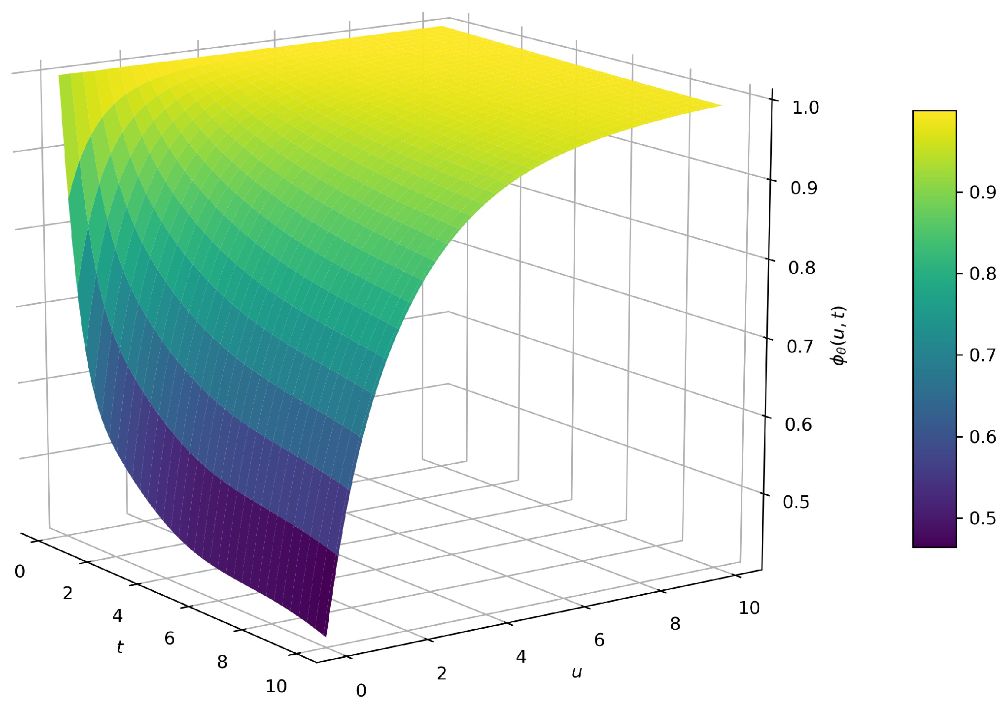
Figure 4 shows the finite-time survival probability calculated by the DNN approximation method after 50,000 iterative calculations, and when using Simpson’s rule to process the integral term, we set ${\delta }_u=0.05$. From the image of the numerical solution, we know that the approximate solution obtained by the deep neural network method is consistent with our expected results. Figure 5 and Figure 6 show the errors between the approximate solutions and exact solutions after 50,000 times of training of two groups of different neural network parameters. We can see that under Parameter 1, the errors between the value calculated by DNN method after 50,000 times of training and the exact solution range from 0 to 0.0015; under Parameter 2, the error range is roughly between 0 and 0.001. On the whole, the error in Figure 6 is smaller. Combined with the results in Figure 5 and Figure 6, and

Table 1. Approximated finite-time survival probabilities with exponential claims for different time horizons $(t=1,3,5,7,9,10)$ with various initial reserves $(u=0,1,2,10)$.

		$\mathit{t}=1$	$\mathit{t}=3$	$\mathit{t}=5$	$\mathit{t}=7$	$\mathit{t}=9$	$\mathit{t}=10$
$u=0$	(1)	0.5366	0.3448	0.2804	0.2457	0.2232	0.2146
	(2)	0.5343	0.3429	0.2785	0.2437	0.2212	0.2126
	(3)	0.5360	0.3385	0.2763	0.2457	0.2196	0.2174
	(4)	0.5401	0.3526	0.2876	0.2505	0.2257	0.2121
	(5)	0.5369	0.3450	0.2804	0.2458	0.2233	0.2147
	(6)	0.5364	0.3445	0.2803	0.2455	0.2226	0.2142
$u=1$	(1)	0.7619	0.5740	0.4881	0.4365	0.4013	0.3874
	(2)	0.7625	0.5740	0.4876	0.4357	0.4001	0.3861
	(3)	0.7624	0.5798	0.4925	0.4341	0.4080	0.3849
	(4)	0.7644	0.5815	0.4926	0.4399	0.465	0.3891
	(5)	0.7591	0.5753	0.4881	0.4368	0.4017	0.3876
	(6)	0.7623	0.5738	0.4877	0.4361	0.4008	0.3871
$u=2$	(1)	0.8803	0.7315	0.6456	0.5886	0.5475	0.5309
	(2)	0.8809	0.7318	0.6453	0.5880	0.5465	0.5297
	(3)	0.8798	0.7336	0.6383	0.5931	0.5460	0.5371
	(4)	0.8842	0.7374	0.6483	0.5943	0.5507	0.5322
	(5)	0.8801	0.7315	0.6452	0.5882	0.5472	0.5306
	(6)	0.8801	0.7315	0.6453	0.5884	0.5473	0.5308
$u=10$	(1)	0.9997	0.9968	0.9908	0.9826	0.9731	0.9681
	(2)	0.9994	0.9968	0.9908	0.9827	0.9731	0.9681
	(3)	0.9999	0.9971	0.9921	0.9813	0.9742	0.9688
	(4)	0.9999	0.9986	0.9927	0.9846	0.9765	0.9713
	(5)	0.9999	0.9973	0.9916	0.9827	0.9753	0.9705
	(6)	0.9999	0.9964	0.9906	0.9823	0.9731	0.9679

, we can see that the more layers there are in the neural network and the higher the number of neurons in each layer, the more accurate the calculation results are. However, the more complex the network structure is, the more resources are consumed in the calculation. Therefore, in order to balance the accuracy of the calculation results, the time needed for program calculation, and the computational resources consumed, a more appropriate set of parameters needs to be selected, which usually requires the experimenter to have enough experience.

The key points of Table 1 are as follows:

(1)

gives the exact values of the finite-time survival probabilities;

(2)

denotes the values of the survival probabilities computed by using the multinomial lattice approximate method proposed by [15] with $\Delta h=0.01$;

(3)

represents the values calculated by the Monte Carlo simulation with 10,000 path and $\Delta t=0.01$;

(4)

represents the values calculated by the nonparametric estimation (see [21]) with 10,000 data points;

(5)

denotes the values computed by using the DNN method with parameter 1;

(6)

denotes the values computed by using the DNN method with parameter 2.

Example 2. 

Considering the classical risk model as described in Equation (1), we assume that the individual claim size follows Pareto distribution with parameter $k=4,x_{min}=2$, the premium income is $c=1.1$, and the parameter of the Poisson process is $\lambda =1$.

$$\begin{array}{c}\hfill p(x)=\left\{\begin{array}{cc}0,\hfill & ifx\le x_{min},\hfill \\ \\ {\displaystyle \frac{k{x}_{min}^k}{x^{k+1}}},\hfill & ifx>x_{min}.\hfill \end{array}\right.\end{array}$$

Figure 7 shows the approximations of survival probability calculated by the DNN method when the individual claim function is a Pareto distribution. It can be seen from the figures that when t is fixed, the probability of survival increases when the initial surplus level u increases, and when u is fixed, the probability of survival decreases as t increases.

The key points of

Table 2. Approximated finite-time survival probabilities with Pareto claim size for different time horizons $(t=1,3,5,7,9,10)$ with various initial reserves $(u=0,1,2,10)$.

		$\mathit{t}=1$	$\mathit{t}=3$	$\mathit{t}=5$	$\mathit{t}=7$	$\mathit{t}=9$	$\mathit{t}=10$
$u=0$	(1)	0.6240	0.4977	0.4569	0.4361	0.4236	0.4191
	(2)	0.6260	0.5020	0.4460	0.4351	0.4283	0.4164
	(3)	0.6306	0.5061	0.4521	0.4326	0.4265	0.4206
	(4)	0.6258	0.5019	0.4518	0.4363	0.4246	0.4132
	(5)	0.6254	0.5016	0.4523	0.4358	0.4241	0.4146
$u=1$	(1)	0.8701	0.7666	0.7212	0.6956	0.6793	0.6732
	(2)	0.8710	0.7709	0.7229	0.6999	0.6776	0.6774
	(3)	0.8732	0.7724	0.7219	0.6987	0.6761	0.6754
	(4)	0.8680	0.7652	0.7173	0.6933	0.6779	0.6692
	(5)	0.8692	0.7659	0.7187	0.6942	0.6773	0.6714
$u=2$	(1)	0.9451	0.8788	0.8425	0.8199	0.8048	0.7990
	(2)	0.9430	0.8775	0.8397	0.8183	0.8075	0.8017
	(3)	0.9418	0.8793	0.8375	0.8214	0.8061	0.8028
	(4)	0.9431	0.8771	0.8398	0.8174	0.8029	0.7965
	(5)	0.9438	0.8774	0.8407	0.8186	0.8043	0.7987
$u=10$	(1)	0.9989	0.9972	0.9952	0.9933	0.9916	0.9909
	(2)	0.9997	0.9987	0.9946	0.9941	0.9911	0.9902
	(3)	0.9995	0.9991	0.9968	0.9943	0.9897	0.9877
	(4)	0.9989	0.9967	0.9944	0.9925	0.9910	0.9904
	(5)	0.9989	0.9969	0.9947	0.9941	0.9924	0.9917

are as follows:

(1)

denotes the values of the survival probabilities computed by using the multinomial lattice approximate method with $\Delta h=0.01$;

(2)

represents the values calculated by the Monte Carlo simulation with 10,000 path and $\Delta t=0.01$;

(3)

represents the values calculated by the nonparametric estimation with 10,000 data points;

(4)

denotes the values computed by using the DNN method with parameter 1;

(5)

denotes the values computed by using the DNN method with parameter 2.

5.2. $\tau (u,t)\ne 0$

When $\tau (u,t)=\lambda [\overline{P}(u)-\overline{P}(u+y)]$, the problem becomes how to find the joint distribution function (df) of the ruin time and the deficit at ruin. The joint df satisfies the equation,

$$\begin{array}{cc}\hfill \frac{\partial }{\partial t}{G}_{\theta }(u,y,t)=& c\frac{\partial }{\partial u}{G}_{\theta }(u,y,t)-\lambda G_{\theta }(u,y,t)\hfill \\ \hfill & +\lambda {\int }_0^u{G}_{\theta }(u-x,y,t)p(x)dx+\lambda [\overline{P}(u)-\overline{P}(u+y)].\hfill \end{array}$$

(28)

Then, we use DNN method to solve Equation (28) under the classical risk model. For the following examples with different claim size distributions, we use a network architecture as follows: 4 hidden layers, each layer has 8 neurons, and the activation function is the tanh function. In order to ensure the accuracy of parameter convergence and improve the speed of parameter updating iteration, we adopt a piecewise learning rate instead of a fixed learning rate

$$\eta (n)=0.01{\mathbf{1}}_{\{n<1000\}}+0.001{\mathbf{1}}_{\{1000\le n<3000\}}+0.0005{\mathbf{1}}_{\{3000\le n\}},$$

where $\eta (n)$ means that for the step size in the gradient descent type algorithm, the first 1000 steps use a learning rate of 0.01; from 1000 to 3000 the learning rate = 0.001; from 3000 onward, the learning rate = 0.0005, which decays in a piecewise constant fashion, and we set up a “tf.keras.optimizer” to train the model.

Example 3. 

We assume that individual claims follow an exponential distribution with the same parameters as Example 1.

Example 4. 

We assume that individual claims follow a Pareto distribution with the same parameters as Example 2.

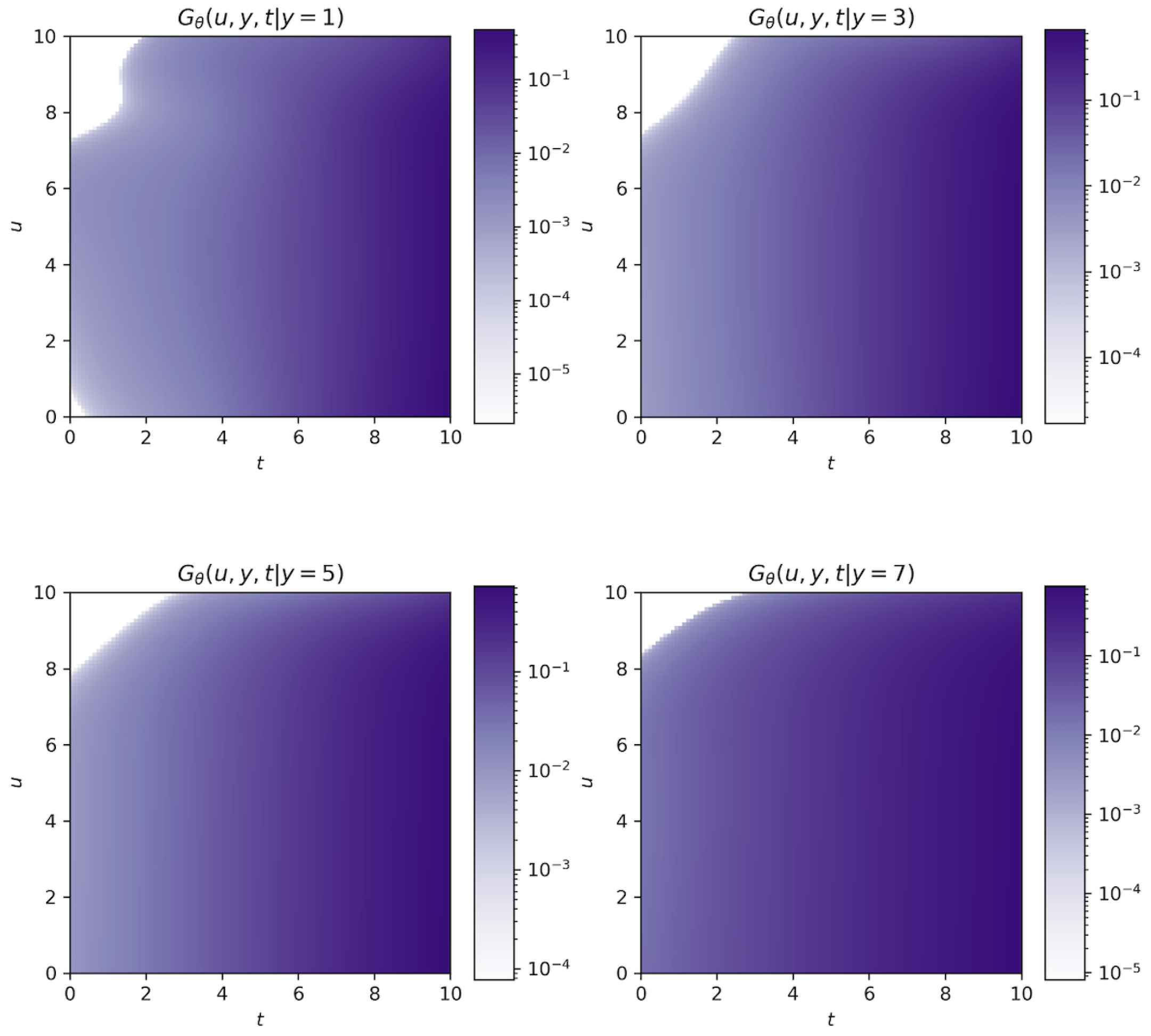
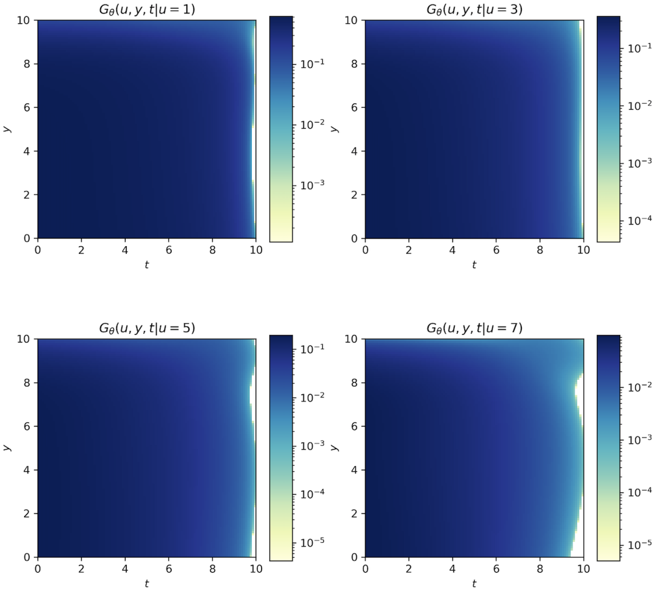
Firstly, the training data set is constructed and letting $(u,y,t)=[0,10]\times (0,10]\times [0,10]$, we randomly select 200 data points according to uniform distribution in the region and then select 30 points on the initial value $t=0$, that is, $D_E=200$, $D_I=30$. The data collected to construct the training data set for solving Equation (28) are shown in Figure 8. The data points at $t=0$ are represented by a red ’x’, and the data samples inside the region are represented by black dots. All data points are randomly sampled. Figure 9, Figure 10 and Figure 11 are the numerical simulation results of Example 3, and Figure 12, Figure 13 and Figure 14 are the results of Example 4.

Figure 9 is the approximate solution obtained when y is fixed. We know that as y goes to infinity, $G(u,y,t)$ degenerates into the distribution of ruin time. Therefore, if y and u are constant, the value of $G(u,y,t)$ should increase as t increases; if y and t are fixed, the value of $G(u,y,t)$ decreases as u increases. This is consistent with the numerical simulation results in Figure 9; with the increase in y or t, the color in the region gradually deepens, which means that the value of the joint distribution $G_{\theta }$ keeps increasing.

Figure 10 shows the numerical solution when t is fixed. As can be seen from the four subgraphs from the top left to the bottom right, under the condition that u and y remain unchanged, the overall color of the figures are deepened with the increase in t, that is, the numerical result of $G(u,y,t)$ becomes larger with the increase in time. This is the same as the theory that the longer the period of time, the greater the probability of bankruptcy, and when $t=0$, the ruin probability is 0. With other things being equal, the smaller the amount of initial capital, the greater the ruin probability. The numerical results given in Figure 11 also confirm the fact that as u increases, the value of $G(u,y,t)$ decreases. In other words, as u increases, the color in the region gradually becomes lighter, that is, the corresponding joint distribution value also decreases.

In Figure 12, Figure 13 and Figure 14, we use the DNN method to give numerical solutions of the joint distribution of ruin time and the deficit at ruin $G(u,y,t)$ with a Pareto claim distribution. Figure 12 shows that with the increase in t, the value of $G(u,y,t)$ also increases, that is, the longer the time, the greater the ruin probability. This result is similar to that of the exponential distribution; moreover, the results shown in Figure 13 and Figure 14 are the same as those obtained for the exponential claim size (Figure 10 and Figure 11). According to the results in Figure 9, Figure 10 and Figure 11, we can see that deep learning is also suitable for solving high-dimensional problems. After setting an appropriate network structure, more accurate results can also be obtained after repeated network training.

It can be seen from the results in

Table 3. The CPU time of the DNN method under different parameters and training times ($D_E=200$, $D_I=30$).

	$\mathit{N}=1000$	$\mathit{N}=5000$	$\mathit{N}=$ 10,000	$\mathit{N}=$ 50,000	$\mathit{N}=$ 100,000
Parameter 1	56 s	248 s	515 s	2480 s	4560 s
Parameter 2	146 s	569 s	1074 s	5690 s	10,456 s

and

Table 4. The CPU time of the DNN method with alternative formulae ($D_E=200$, $D_I=30$).

Training Times	$\mathit{N}=1000$	$\mathit{N}=5000$	$\mathit{N}=$ 10,000	$\mathit{N}=$ 50,000	$\mathit{N}=$ 100,000
Parameter 1	2 s	5 s	9 s	42 s	81 s
Parameter 2	3 s	14 s	28 s	135 s	278 s

that the calculation time consumed by the deep neural network in training data sets is positively correlated with the total number of training times. When Simpson’s discretization is used to deal with the integral term, the calculation time is greater, and if the replacement formula is used, the calculation time is greatly reduced.

Table 5. The CPU time of the Monte Carlo method under different paths.

Path Number	$\mathit{N}=1000$	$\mathit{N}=5000$	$\mathit{N}=$ 10,000	$\mathit{N}=$ 50,000	$\mathit{N}=$ 100,000
$\Delta t=0.01$	1 s	6 s	15 s	83 s	205 s
$\Delta t=0.001$	8 s	36 s	76 s	452 s	1104 s

shows the CPU time of the Monte Carlo method under different path number settings when $\Delta t=0.01$ and $\Delta t=0.001$. It is worth mentioning that the results obtained by the DNN method are not for a single data point $(u_i,t_i)$; rather, for a given whole interval $u\times t=[0,10]\times [0,10]$, the plane of the numerical solution is given. The Monte Carlo method and other approximate algorithms can only solve a single data point $(u_i,t_i)$. Based on its calculation efficiency, it can be seen that the DNN method has great advantages.

Moreover, the DNN method has another significant advantage: it does not consume much computer storage space. Random simulation and other approximation algorithms need to split the direction of time and space in the calculation process, so the previous results need to be stored in each calculation, that is, the finer the grid, the greater the required computer storage space. However, the deep neural network method updates the parameters according to each calculation result, that is, there is no need to store all the calculation results, thus greatly reducing the consumption of computer memory resources.

6. Conclusions

In this paper, we presented a new method for solving PIDEs. The newly proposed method uses deep neural networks that are trained iteratively by using gradient descent type algorithms. For the relatively general individual claim distribution, the general Simpson’s rule is used to discretize the integral term in the equation. For the exponential claim distribution, the integral term can be eliminated by transformation so as to transform the PIDE into a PDE. This is beneficial for improving the efficiency and accuracy of the calculation in neural network training. Furthermore, due to the effectiveness of neural networks in approximating functions, this method can also be extended to other risk models, such as the risk model with diffusion terms and the Markov arrival process (MAP) risk model in the case of multiple dimensions.

The powerful expressive ability of DNNs enables them to accurately approximate arbitrary functions. The accuracy of the method depends on several aspects: the depth of the network, i.e., the number of hidden layers; the number of neurons in each hidden layer; the iteration step size selection; and the size of the training data set. As we know, when other conditions remain unchanged, the more layers there are in the neural network, the higher the accuracy of its calculation. Similarly, the more neurons on each layer and the larger the size of the training data set, the better the calculation effectiveness of the algorithm.

Although the deep neural network method has great advantages in solving equations, it is very difficult to estimate the error of this method because the parameter updating process is a black box. In addition, there is no theoretical basis for setting the network structure; these decisions rely on the personal experience of researchers.

In the future, we will focus on the deep neural network method for non-local models, as it can approximate any given function with the aid of a nonlinear structure, thus providing a new idea for how to deal with problems in high dimensions. In addition, high-order numerical algorithms and their error analysis in non-local models are also important research directions for us in the future, especially with respect to irregular regions and multi-dimensional problems.

References

1. Klafter, J.; Lim, S.C.; Metzler, R. Fractional Dynamics: Recent Advances; World Scientific: Singapore, 2011. [Google Scholar]
2. Klages, R.; Radons, G.; Sokolov, I.M. Anomalous Transport; Wiley: New York, NY, USA, 2008. [Google Scholar]
3. Shlesinger, M.F.; Zaslavsky, G.M.; Frisch, U. Lévy Flights and Related Topics in Physics; Springer: Berlin/Heidelberg, Germany, 1995. [Google Scholar]
4. Dickson, D.C. The joint distribution of the time to ruin and the number of claims until ruin in the classical risk model. Insur. Math. Econ. 2012, 50, 334–337. [Google Scholar] [CrossRef]
5. Dickson, D.C.; Willmot, G.E. The density of the time to ruin in the classical Poisson risk model. ASTIN Bull. J. IAA 2005, 35, 45–60. [Google Scholar] [CrossRef] [Green Version]
6. Drekic, S.; Willmot, G.E. On the density and moments of the time of ruin with exponential claims. ASTIN Bull. J. IAA 2003, 33, 11–21. [Google Scholar] [CrossRef] [Green Version]
7. Li, S.; Lu, Y. Distributional study of finite-time ruin related problems for the classical risk model. Appl. Math. Comput. 2017, 315, 319–330. [Google Scholar] [CrossRef]
8. Constantinescu, C.; Samorodnitsky, G.; Zhu, W. Ruin probabilities in classical risk models with gamma claims. Scand. Actuar. J. 2018, 7, 555–575. [Google Scholar] [CrossRef]
9. Avram, F.; Usabel, M. Finite time ruin probabilities with one Laplace inversion. Insur. Math. Econ. 2003, 32, 371–377. [Google Scholar] [CrossRef] [Green Version]
10. Dickson, D.C. A note on some joint distribution functions involving the time of ruin. Insur. Math. Econ. 2016, 67, 120–124. [Google Scholar] [CrossRef]
11. Willmot, G.E. On a partial integrodifferential equation of Seal’s type. Insur. Math. Econ. 2015, 62, 54–61. [Google Scholar] [CrossRef]
12. DeVylder, F.E.; Goovaerts, M.J. Explicit finite-time and infinite-time ruin probabilities in the continuous case. Insur. Math. Econ. 1999, 24, 155–172. [Google Scholar] [CrossRef]
13. Chen, M.; Yuen, K.C.; Guo, J. Survival probabilities in a discrete semi-Markov risk model. Appl. Math. Comput. 2014, 232, 205–215. [Google Scholar] [CrossRef]
14. Lefevre, C.; Loisel, S. Finite-time ruin probabilities for discrete, possibly dependent, claim severities. Methodol. Comput. Appl. Probab. 2009, 11, 425–441. [Google Scholar] [CrossRef] [Green Version]
15. Costabile, M.; Massabo, I.; Russo, E. Computing finite-time survival probabilities using multinomial approximations of risk models. Scand. Actuar. J. 2015, 5, 406–422. [Google Scholar] [CrossRef]
16. Picard, P.; Lefevre, C. The probability of ruin in finite time with discrete claim size distribution. Scand. Actuar. J. 1997, 1997, 58–69. [Google Scholar] [CrossRef]
17. Dickson, D.C.; Waters, H.R. Ruin probabilities with compounding assets. Insur. Math. Econ. 1999, 25, 49–62. [Google Scholar] [CrossRef]
18. Cheung, E.C.; Zhang, Z. Simple approximation for the ruin probability in renewal risk model under interest force via Laguerre series expansion. Scand. Actuar. J. 2021, 2021, 804–831. [Google Scholar] [CrossRef]
19. Shimizu, Y. Non-parametric estimation of the Gerber-Shiu function for the Wiener-Poisson risk model. Scand. Actuar. J. 2012, 2012, 56–69. [Google Scholar] [CrossRef]
20. Zhang, Z. Estimating the Gerber-Shiu function by Fourier-Sinc series expansion. Scand. Actuar. J. 2017, 2017, 898–919. [Google Scholar] [CrossRef]
21. Zhang, Z. Nonparametric estimation of the finite time ruin probability in the classical risk model. Scand. Actuar. J. 2017, 2017, 452–469. [Google Scholar] [CrossRef]
22. Raissi, M.; Perdikaris, P.; Karniadakis, G.E. Physics-informed neural networks: A deep learning framework for solving forward and inverse problems involving nonlinear partial differential equations. J. Comput. Phys. 2019, 378, 686–707. [Google Scholar] [CrossRef]
23. Raissi, M.; Perdikaris, P.; Karniadakis, G.E. Physics informed deep learning (part i): Data-driven solutions of nonlinear partial differential equations. arXiv 2017, arXiv:1711.10561. [Google Scholar]
24. Beck, C.; Becker, S.; Grohs, P.; Jaafari, N.; Jentzen, A. Solving stochastic differential equations and Kolmogorov equations by means of deep learning. arXiv 2018, arXiv:1806.00421. [Google Scholar]
25. Van der Meer, R.; Oosterlee, C.W.; Borovykh, A. Optimally weighted loss functions for solving pdes with neural networks. J. Comput. Appl. Math. 2022, 405, 113887. [Google Scholar] [CrossRef]
26. Weinan, E.; Han, J.; Jentzen, A. Deep learning-based numerical methods for high-dimensional parabolic partial differential equations and backward stochastic differential equations. Commun. Math. Stat. 2017, 5, 349–380. [Google Scholar]
27. Chen, Y.; Yu, H.; Meng, X.; Xie, X.; Hou, M.; Chevallier, J. Numerical solving of the generalized Black-Scholes differential equation using Laguerre neural network. Digit. Signal Processing 2021, 112, 103003. [Google Scholar] [CrossRef]
28. Blanka, H.; Muguruza, A.; Tomas, M. Deep learning volatility: A deep neural network perspective on pricing and calibration in (rough) volatility models. Quant. Financ. 2021, 21, 11–27. [Google Scholar]
29. Salvador, B.; Oosterlee, C.W.; van der Meer, R. Financial option valuation by unsupervised learning with artificial neural networks. Mathematics 2021, 9, 46. [Google Scholar] [CrossRef]
30. Huh, J. Pricing options with exponential Lévy neural network. Expert Syst. Appl. 2019, 127, 128–140. [Google Scholar] [CrossRef] [Green Version]
31. You, H.; Yu, Y.; D’Elia, M.; Gao, T.; Silling, S. Nonlocal kernel network (nkn): A stable and resolution- independent deep neural network. arXiv 2022, arXiv:2201.02217. [Google Scholar]
32. Chen, H.; Yu, Y.; Jaworski, J.; Trask, N.; D’Elia, M. Data-driven learning of Reynolds stress tensor using nonlocal models. Bull. Am. Phys. Soc. 2021, 66. Available online: https://meetings.aps.org/Meeting/DFD21/Session/E11.2 (accessed on 23 February 2022).
33. Pang, G.; Lu, L.; Karniadakis, G.E. fPINNs: Fractional physics-informed neural networks. SIAM J. Sci. Comput. 2019, 41, A2603–A2626. [Google Scholar] [CrossRef]
Figure 1. Illustration of a neural network with three hidden layers.
Mathematics 10 01504 g001
Figure 2. The data transmission process of a neural network that contains three hidden layers.
Mathematics 10 01504 g002
Figure 3. The randomly selected data points used to construct the training data set.
Mathematics 10 01504 g003
Figure 4. The DNN approximation solution for parameter 1.
Mathematics 10 01504 g004
Figure 5. The error between DNN approximation for parameter 1 and the explicit solution.
Mathematics 10 01504 g005
Figure 6. The error between DNN approximation for parameter 2 and the explicit solution.
Mathematics 10 01504 g006
Figure 7. The DNN approximation solution with a Pareto distribution (the times of training: 50,000).
Mathematics 10 01504 g007
Figure 8. The randomly selected data points used to construct the training data set.
Mathematics 10 01504 g008
Figure 9. The values of G θ ( u , y , t ) for a fixed y (exponential distribution).
Mathematics 10 01504 g009
Figure 10. The values of G θ ( u , y , t ) for a fixed t (exponential distribution).
Mathematics 10 01504 g010
Figure 11. The values of G θ ( u , y , t ) for a fixed u (exponential distribution).
Mathematics 10 01504 g011
Figure 12. The values of G θ ( u , y , t ) for a given y (Pareto distribution).
Mathematics 10 01504 g012
Figure 13. The values of G θ ( u , y , t ) for a given t (Pareto distribution).
Mathematics 10 01504 g013
Figure 14. The values of G θ ( u , y , t ) for a given u (Pareto distribution).
Mathematics 10 01504 g014