1. Introduction
The purpose of classification based on test results is to produce useful information regarding examinees. Since the use of cut scores to classify examinees is widely used, particularly in educational assessment, estimating the statistical performance of classifiers is a vital part of psychometric analysis. Classifications resulting from test cut scores can be dichotomous (e.g., pass or fail) or polytomous (e.g., far below benchmark, below benchmark, at benchmark, above benchmark) depending on the purpose and characteristics of the tests. Regardless, the essential purpose of the assessments is to produce interpretive meaning based upon an examinee’s obtained score with reference scores (e.g., cut-off score) [
1]. For widely used licensure tests (e.g., the Praxis tests, General Educational Development tests), pass/fail distinctions are often the final form of score reporting upon which stakes are based. High stakes decisions are also part of primary and secondary education. For example, the federal grant program entitled “Race to the Top” [
2] emphasizes the accountability and instructional improvement of K-12 assessments, which typically result in classifying students by achievement and reflects the growing importance of improving the quality of classification and the interpretations based on classifications in education.
Classification using examinees’ observed scores is an attempt to accurately categorize continuous quantities into several different groups, dependent on the cut-off scores. Classifying different groups of students in educational settings based on academic or social/behavioral assessments is critical in order to identify students in need of additional supports. For example, research suggests that students performing well below established achievement benchmarks, such as those used in the Dynamic Indicators of Early Literacy Skills (DIBELS) [
3], are at risk for long-term negative outcomes, including grade retention and school drop-out [
4]. Therefore, educators need accurate and reliable classification systems, based on assessment cut scores, to prevent negative outcomes and deliver necessary remediation to increase the likelihood of student success [
5].
Cut-off scores have been successfully identified and used in educational assessments through various procedures [
6,
7,
8]. Traditionally, the quality of the cut-off score has been evaluated by the use of accuracy and consistency of classification results with two indices: (a) classification accuracy (CA) and (b) classification consistency (CC) [
9]. While reporting CA and CC is becoming a common practice, there has been limited research addressing some of the inherent limitations of the two indices. One of the most important threats to the appropriate use of CA and CC indices is unbalanced class distribution. In practice, the numbers of individuals in different classes can vary greatly, which causes problems when focusing exclusively on correct classes, as do the CC and CA indices [
10].
Another limitation of the CA and CC indices is that they fail to show the varying performance of the classifier across the whole group. Let us consider the illustrated example in
Table 1. In Case 1, a small number of examinees have actual failing status according to the cut score and yet the classifier placed all examinees into the passing group. CA would equal 80%, and this may be misleading because all examinees who should have been in the failing category were misclassified. In other words, the classifier does not perform well for examinees with lower abilities. In Case 2, the CA is again 80% and the distribution of actual classification groups is more balanced. However, the classifier does not perform well for examinees with higher abilities. Given that the goal of many educational assessments is to classify and identify a small group of students at risk, often to deliver necessary intervention, CA indices are concerning because the value can be the same even when the pattern of results are different, as was the circumstance in Case 1 and Case 2.
Since CC and CA are often poor metrics for measuring classification quality, other indices have been developed as alternatives. Specifically, the use of receiver operating characteristics (ROC) graphs is increasingly being used for estimating and visualizing the performance of classifiers [
11,
12]. Applying the ROC approach to educational assessment not only mitigates the limitations of CA and CC, but also provides more information about the performance of classifiers beyond CA and CC. However, few research have been conducted applying ROC despite the advantage of giving quality information regarding the classification. It is not as widely used to evaluate students’ knowledge and skills [
13] though the ROC has been widely used in various disciplines including medical or clinical settings for diagnostic purposes [
14,
15,
16,
17]. As such, the goal of this paper is to introduce the ROC graph as a means to overcome the limitations of CA and CC indices in educational assessment. Specifically, this study will demonstrate how the ROC approach is able to depict the tradeoff between benefits (i.e., true positive rate) and costs (i.e., false positive rate) in classification through simulation study. Below, the author will provide the theoretical background and use simulated data to show that the ROC functions well across various test conditions, including test length, sample size, and distribution of students’ ability.
2. Theoretical Background
2.1. Classification Accuracy and Classification Consistency
Definition of Classification Accuracy and Classification Consistency
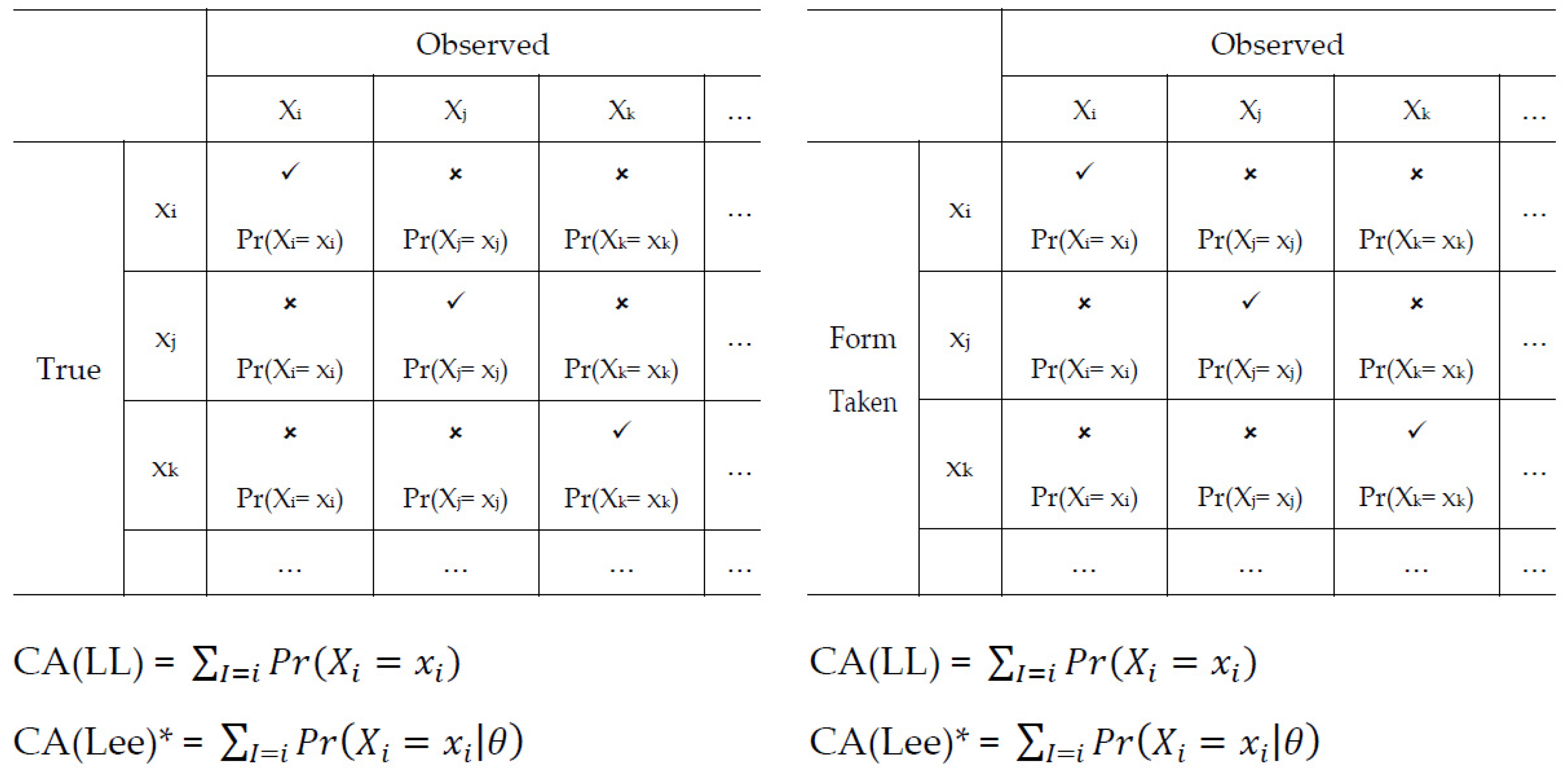
Classification accuracy (CA) is the rate at which the classifications based on observed cut scores agree with classifications based on true cut scores [
9,
18]. Classification consistency (CC) is the rate at which examinee classifications based on repeated independent and parallel test forms agree with each other [
19]. There are two approaches that are commonly used to estimate CA and CC—the Livingston and Lewis approach [
18], using the beta distribution, and the Lee approach [
9], using the IRT framework—provided in
Figure 1.
The most widely used approach to estimate CA and CC is the Livingston and Lewis (LL) approach [
9,
20,
21,
22,
23,
24]. This approach has been used in a number of high stakes education assessment systems, including the California Standards Tests, the Florida Comprehensive Assessment Test, and the Washington Comprehensive Assessment Program.
Another way of estimating CA and CC is the Lee’s approach developed using the item response theory (IRT) framework [
18,
19,
22,
25,
26]. Lee’s approach has also been used in high stakes assessment systems, including the Connecticut Mastery Test. This approach first employs a compound multinomial distribution [
27] to model the conditional summed-score distribution and aggregate the probabilities of scoring with a given category. Then, CA and CC are calculated using an
n by
n contingency table, similar to the LL approach.
2.2. Classification Matrix and ROC Graph
2.2.1. Classification Matrix
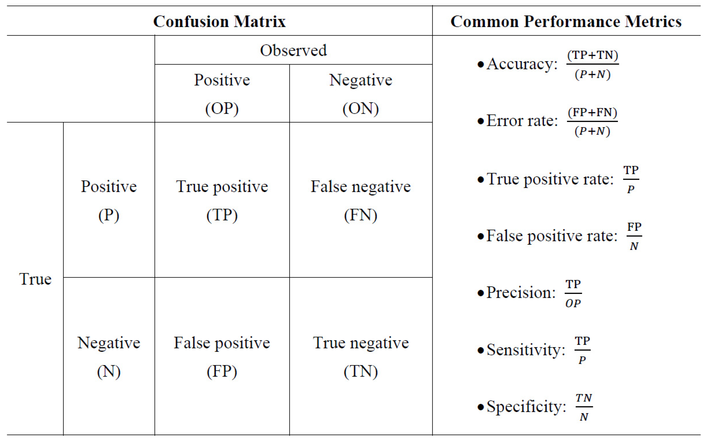
Classification matrix is constructed by using two classes, positive and negative, which can be regarded as “pass” and “fail” in real cases. The information on the true positive rate and the false positive rate can be computed using a 2-by-2 confusion matrix.
Figure 2 shows a classification matrix and equations for several commonly used metrics that can be calculated from it.
True positive signifies that a positive examinee is correctly classified as positive.
False negative indicates that a positive examinee is misclassified as negative.
False positive means that a negative examinee is misclassified as positive. Finally,
true negative means that a negative examinee is correctly classified as negative.
There are more indices that can be estimated using the classification matrix, including negative predictive value, miss rate, false discovery rate and so on. This study focuses on the true positive rate and the false positive rate here as they are typically the values of interest. The true positive rate can be interpreted as the probability of positives that are correctly classified among all the positives, and the false positive rate can be interpreted as the probability of negatives that are incorrectly classified as positives among all the negatives.
2.2.2. ROC Graph
ROC graphs are built with the true positive rate plotted on the
y-axis and treated as a benefit, and false positive rate plotted on the
x-axis and treated as a cost [
28]. To estimate the classification quality in a test, it is necessary to plot costs and benefits in the ROC space. When examinees are classified in a test, only a single classification matrix can be generated based on the cut score, which corresponds to one single point in the ROC space. The single point represents the overall performance of a classifier.
In addition to the single point, this study also focuses on plotting a curve to reflect the performance of the classifier across different cut score locations. The ROC curve consists of the entire set of false positive rate and true positive rate pairs (i.e., cost–benefit) resulting from the continually changing cut scores over the range of test results, plotting the changing cut scores, and therefore it has been recognized as a global measure of a test’s accuracy [
29].
The cost–benefit approach uses the ROC graph to generalize information from the tradeoffs between false and true positives.
Figure 3 shows the ROC graph where each point in the ROC space represents a classifier’s performance.
A classifier at the lower left point O (0, 0) means that both cost and benefit are equal to 0. A classifier at the upper right point C (1, 1) means that both cost and benefit are equal to 1. A classifier at the upper left point B (0, 1) means that the cost is 0 and the benefit is 1, representing perfect classification. Intuitively, a classifier has better performance if its points in the ROC space are close to point B, where benefits are high, and costs are low. The diagonal line represents random performance because it means the classifier has a 50% chance of correctly classifying examinees into either positive or negative.
2.3. Use of the ROC to Estimate Classification Quality in Practice
The development of classification quality was inspired by the idea that both correctly classified examinees and those who are incorrectly classified should be considered to evaluate the performance of the classifier. Classification quality is the attribute of a classifier that portrays the relationship between the classifications based on observed cut scores and the classifications based on true cut scores. Accuracy and consistency indices have been computed for decades in the context of educational assessment, and the newly proposed classification quality serves as an alternative to alleviate some problems of the traditional indices.
One of the inherent problems of the accuracy and consistency indices is their unbalanced class distribution. In fact, any performance metric that uses values from multiple columns (e.g., “pass” and “fail”) is inherently sensitive to class skews [
30,
31]. Even if the performance of the classifier does not change, the variation in class distribution changes the accuracy index because it is computed across multiple columns. ROC curves are different from other indices because they use a row-parallel computation using the classification. The true and false positive rates are ratios from two columns without crossing rows; therefore, the ROC curve is insensitive to class distributions. In practice, it is not unusual to see that less than 15% of respondents are classified into “fail” in many assessments based on a cut score [
32], and this causes unbalanced class distribution. Another attractive feature of using ROC graphs is that they provide a tradeoff between costs and benefits across all cut scores in the sample. ROC graphs can uncover potential reasons behind the varied classification quality with the change in cut scores and can provide a visual display of the variation.
In this study, the area under the curve (
AUC) is used to quantify cost–benefit. The
AUC is the probability that a classifier will rank a randomly chosen positive instance higher than a negative one [
33]. AUC is also equal to the value of the Wilcoxon-Mann–Whitney U test statistic. Basically,
AUC is calculated based on the true positive rate and false positive rate. Formally,
AUC given a cut score at
i can be computed as Equation (1).
where
TPR denotes true positive rate
,
FPR denotes false positive rate
,
denotes the sum of ranks. The
AUC can be easier to calculate using the Gini coefficient [
34] by
, given
is computed as
Although
AUC has a range between 0 to 1 in the
ROC space, it is mentioned that a classifier should perform no worse than random guessing, which means that a classifier in real practice is expected to have an
AUC > 0.5. In general, an AUC of 0.7 to 0.8 is considered acceptable, 0.8 to 0.9 is considered excellent, and more than 0.9 is considered outstanding [
35].
In summary, ROC graphs overcome the shortcomings of using accuracy indices and produce more detailed information on classification quality. In addition, multiple indices can be generated using classification matrices. Of those, AUC is a useful and informative indicator in cost–benefit analysis.
3. Method
A simulation study was conducted to investigate factors that might influence classification quality. Based on the literature reviews in psychometric simulation studies, factors were manipulated including sample size, test length, and distribution of ability [
36,
37,
38,
39,
40]. In this study, the factors are specified as follows: test length (i.e., 20, 40, and 60 items), ability distributions (i.e., a normal distribution, a skewed distribution, and a mixed distribution), and sample size (i.e., 500, 1000, and 3000). Each condition was replicated 50 times.
In order to reflect practical settings, the true item parameters for the various simulated tests were taken from an operational, high-stakes test in the state of Florida. All items are binary scored, and the relationship between item parameters and the probability of correct response followed a 3-parameter logistic (3PL) model with difficulty, discrimination, and lower-asymptote parameters,
[
41]. Specifically, 6th grade mathematic results are used to generate the simulated item parameters. The parameter estimation results are reported in an annual technical report (Florida Comprehensive Assessment Test, 2006), and item parameter estimate is summarized in
Table 2.
The range of the item discrimination estimates is from approximately 0.44 to 1.39. For difficulty parameters, the range is from −1.82 to 1.6. For lower-asymptote parameter, the range is 0.07 to 0.33. Using these parameter estimates, we generated the item parameters for the simulation. Specifically, the discrimination parameter was sampled from a uniform distribution with a range of (0.44, 1.39). The difficulty parameter was sampled from a uniform distribution with a range of (−1.82, 1.60). For the lower-asymptote parameter, the parameter was sampled from a uniform distribution with a range of (0.07, 0.33).
Abilities were drawn from three types of different ability distributions: (a) normal distribution, (b) Fleishman distribution, and (c) mixed distribution. Under the normal distribution, true ability followed a standard normal distribution. The data generation under the skewed condition followed Fleishman [
37], where the ability distribution has mean 0, standard deviation 1, skewness 0.75, and kurtosis 0. In the mixed condition, ability came from two normal distributions
(−0.25, 0.61) and
(2.19, 1.05) with mixing proportion of 90% and 10%, respectively, which also has a mean 0 and standard deviation 1, as used in Woods [
40].
To form ROC curves, results within each individual data set were aggregated across the 50 replications for each condition. Threshold averaging was used to aggregate across replications where both true positive rates and false positive rates were averaged at fixed intervals [
42]. AUC were also calculated and reported for all ROC graphs.
Using generated item parameters and abilities, the response vectors were generated using the R package
cacIRT. Using generated response vectors, we performed AUC calculation and ROC construction in the R package
ROCR. R version 4.0.2 was used to perform the simulation [
43].
4. Results
Figure 4a–i show how the ROC curves change with different test lengths (i.e., 20, 40, and 60 items) and sample size (i.e., 500, 1000, and 3000) when the ability distributions are normal, skewed, and mixed, respectively. Further, the figures show the performances of the different classifiers, and since 50 replications per each condition were performed, 50 graphs are depicted for each condition because each graph represents a single replication. Thus, graphs are depicted in each plot.
Figure 4a–c show the trend of ROC curves with different test lengths under different ability distributions. The three graphs show the effects of test length by comparing the performance among the classifiers.
Figure 4d–f show the trend of ROC curves with different ability distributions under different test lengths. The three graphs show the effects of the ability distribution by comparing the performance among the classifiers.
Figure 4g–i show the trend of ROC curves with different sample sizes under different ability distributions. The three graphs show the effects of sample size by comparing performance among the classifiers.
Specifically, the results of the comparison of the performances of the classifiers based on AUC and cut-off score with sensitivity and specificity are reported in
Table 3 and
Table 4 in the following section.
Results for average AUCs through replications and how the AUC changes with test length, sample size, and ability distribution are presented in
Table 3.
Table 3 shows that the use of ROC works outstanding for all conditions with AUC as Han, Pei, and Kamber’s [
35] suggestions (i.e., all AUCs > 0.9). AUC is the largest when the ability distribution is skewed, the second largest when examinees’ ability distribution is normal, and the smallest when the ability distribution is mixed. This suggests that the classifier works best when the ability distribution is skewed. Results also shows that AUC increases with longer test length, as confirmed with ANOVA through 50 replications. However, the impact of sample size was indistinguishable (which was, again, confirmed with ANOVA procedures). Although AUC indices give us the comprehensive performance of the classifier under each condition, the specific differences under each condition can be better seen in
Table 4 in the following section.
The results in
Table 4 provide the cut-off score, sensitivity, and specificity. One of the most distinctive trends is that when the number of items is increased, the cut-off score tends to decrease. Additionally, sensitivity and specificity are increased. This trend is applicable to all ability distributions. However, when the number of items is the same, the effect of sample size is indistinguishable. Nonetheless, sensitivity and specificity are the highest when the ability distribution is skewed, and lowest when the ability distribution is mixed.
5. Discussion and Conclusions
Assessment is the systematic process of implementing empirical data to measure knowledge, skills, attitudes, and beliefs. This study introduces a cost–benefit approach that overcomes the problems of using CC and CA methods, as well as provides practitioners with more information about classification quality. The author demonstrated two ways of using the cost–benefit approach to estimate classification quality: (a) plot the ROC point generated by the classification in the ROC space to show the classification performance, and (b) build the ROC curve to show the classification performance across all cut score locations. It is worth mentioning that neither way requires additional statistical analysis of the original dataset, and practitioners with the classification results can easily carry it out. A simulation study was conducted on classification quality. The results show that (a) the use of ROC methodology works well for classification, and (b) longer tests usually produce higher classification quality.
It should be noted that true classification distinctions should be given to applying ROC for evaluating classification quality in practice. For example, one can identify true classification results in marketing settings (e.g., whether or not a customer purchases a product) that are directly observable. This can also happen in medical or clinical settings where one can confirm that a patient has a disease or not through surgery or a pre-existing valid diagnostic instrument. Given a priori decision on classification, ROC can be used in education for evaluating the performance of classifiers under various conditions or among several different methods, as well as determining the optimal cut-point of a particular test. However, unlike other fields, such as marketing, it is challenging to know for certain whether or not examinees truly possess the trait that is intended to be measured in educational or psychological settings. Since many of these traits (e.g., language ability) are unobservable, it is not always possible to know true classification results a priori in practice unless the data come from simulated datasets. This is the fundamental problem of applying ROC in situations of educational assessment or licensure tests.
Notwithstanding the limitations of applying ROC in practice, there are additional research questions to address the usefulness of using ROC in education testing contexts. First, true classification specification might be achieved through cognitive diagnostic modeling (CDM), which leads to the potential use of ROC in determining the optimal cutoff scores of a particular assessment. As long as we can specify reliable confirmed diagnostic results, ROC can be used for evaluating the performance of the assessment as well as determining cutoff scores depending on the purpose of the assessment. Second, in the field of vocational education, it is quite feasible to determine whether a person has a particular skill (i.e., psycho-motor skills) or not regardless of those licensure tests. Based on judgment from true classification results, ROC can be used for evaluating the performance of the assessment as well as determining cutoff scores. In sum, when we want to apply ROC dealing with a latent trait for both scenarios, the core factor is to determine how one can specify whether people truly possess the trait. Future research should consider these aspects and conduct research on the performance of ROC in relation to CDM or psycho-motor skills and how and to what extent we can assure the accuracy of those results.
There are other directions that we would like to address in future research as well. Since there are multiple ways to generate the ROC curve, future research should consider other ways to fit a curve that better estimates classification quality. Another is that binary classification is used to illustrate the ROC curve in this study. Multi-class AUC and ROC curves have been developed in the area of machine learning. It is worth expanding current research to multi-class instances because many educational assessments use multi-classification approaches.
As noted, classifying different groups of students in educational settings based on academic or social/behavioral assessments is critical in order to identify students in need of additional supports. It is believed that the cost–benefit approach described here can help educational researchers and practitioners increase the accuracy of their classification approaches when assessing student performance. Classification of students and teachers is important for making educational and professional decisions, particularly with regard to identification of those in need of early intervention to increase the likelihood of positive future outcomes. By using a ROC approach, educators can ensure that they are correctly identifying those in need and increase broader confidence in the accuracy of their assessments.


