Abstract
In this paper, we focus on the stochastic fractional Kundu–Mukherjee–Naskar equation perturbed in the Stratonovich sense by the multiplicative Wiener process. To gain new elliptic, rational, hyperbolic and trigonometric stochastic solutions, we use two different methods: the Jacobi elliptic function method and the -expansion method. Because of the significance of the Kundu-Mukherjee equation in a magnetized plasma, the obtained solutions are useful in understanding many remarkable physical phenomena. Furthermore, we show the effect of the multiplicative Wiener process on the obtained solutions of the Kundu–Mukherjee–Naskar equation.
Keywords:
fractional Kundu–Mukherjee–Naskar equation; stochastic Kundu–Mukherjee–Naskar equation; Jacobi elliptic function method; (G′/G)-expansion method MSC:
35Q51; 83C15; 60H10; 35A20; 60H15
1. Introduction
In chemistry, physics, engineering, biology, geophysics and climate dynamics, among other fields [1,2,3,4], the advantages of taking random effects in simulating, analyzing, predicting and modeling compound phenomena have been vastly recognized. Moreover, the presence of noises has been shown to give rise to some statistical features and essential phenomena, such as ergodic behavior forced by degenerate noise and a unique invariant measure. Simultaneously, stochastic perturbations in a physical system cannot be prevented, and they can not be neglected in some cases.
On the other hand, fractional differential Equations (FDEs) have been displayed to be more precise than classical one in explaining complex physical phenomena in the real world. FDEs have drawn the interest of scientists and researchers over the last two decades. The principle of fractional derivative has been utilized to define a variety of phenomena, such as viscoelastic materials, signal processing, fluid dynamics porous medium, ocean wave, photonic, electromagnetism, chaotic systems, propagation of waves, optical fiber communication, plasma physics, nuclear physics and others.
It is critical in nonlinear science to determine the analytic solutions of nonlinear evolution partial differential equations. Therefore, several analytical methods have been developed to deal with these sorts of nonlinear problems, such as the Jacobi elliptic function [5,6], perturbation [7,8,9], sine-cosine [10,11], Hirota’s function [12], -expansion [13,14,15], -expansion [16], tanh-sech [17,18], Riccati-Bernoulli sub-ODE [19], Darboux transformation [20], etc.
To get a better degree of quality consistency, we recognize here the following stochastic fractional-space Kundu–Mukherjee–Naskar equation (SFKMNE) perturbed by the multiplicative Wiener process:
where u denotes the optical soliton profile, is the conformable derivative (CD) [21], are positive constants, is the noise strength, is the multiplicative Wiener process in the Stratonovich sense and is the standard Wiener process (SWP).
Kundu and Mukherjee [22] proposed Equation (1) in 2013 with and . It is attained from the fundamental hydrodynamic equations as a two-dimensional nonlinear Schrödinger equation. This Equation (1) can be utilized to explain ion-acoustic waves, oceanic rogue waves and optical fiber wave propagation in a magnetized plasma [23,24,25,26]. Many research works have been focused on Equation (1) to investigate soliton propagation into an optical fiber. As a result, numerous mathematical methods have been used to obtain exact solutions, such as extended trial function [27], trial Equation [28], modified simple Equation [29], Jacobi elliptic functions and Weierstrass [30] and Lie symmetry [31].
We do not investigate here the uniqueness and existence of the solutions, which is a well-known issue (see, for instance [32,33]).
Our motivation in this article is to get the analytical stochastic fractional solutions of the SFKMNE (1). We employ two various techniques, i.e., the Jacobi elliptic function method and the -expansion method, to acquire solutions of elliptic, trigonometric, hyperbolic and rational functions. Furthermore, to examine the influence of the Wiener process on the solutions of SFKMNE (1), we utilize Matlab tools to create 2D and 3D graphs for several of the analytical solutions generated in this work.
The document is organized as follows: In Section 2, we define and give a few properties of the SWP and CD. In Section 3, we employ an appropriate wave transformation to get the wave equation of the SFKMNE (1), while in Section 4, to create the exact solutions of the SFKMNE (1), we use diverse approaches. In Section 5, the influence of the Wiener process on the derived solutions is investigated. The paper ends with a conclusion section.
2. Preliminaries
We present here some definitions and properties of SWP and CD. First, let us define SWP as follows:
Definition 1.
Stochastic process is said to be an SWP if the following conditions hold:
- 1.
- 2.
- is a continuous function of ,
- 3.
- is independent for ,
- 4.
- has a Gaussian distribution with mean 0 and variance .
We should mention that the two most commonly utilized variants of the stochastic integral are Stratonovich and Itô [34]. Modeling problems mainly determine what form is appropriate; even so, once it is chosen, an equivalent equation of the other type can be created using the same solutions. Thus, the the next relation can be used to swap between Itô (denoted by ) and Stratonovich (denoted by ):
where is supposed to be sufficiently regular and is a stochastic process.
Definition 2
([21]). The CD of of order is defined as
Theorem 1
([21]). Let be differentiable, and also let α be a differentiable function, then:
Let us exhibit some features of the CD:
- 1.
- 2.
- , where C is a constant,
- 3.
- 4.
3. Wave Equation for SFKMNE
We use the following wave transformation to obtain the wave equation for the SFKMNE (1):
with:
where is a deterministic function and are nonzero constants for . Plugging Equation (3) into Equation (1) and using:
and:
we get for the imaginary part:
and for the real part:
We get by taking expectation :
To calculate the value of the parameter N, which will be needed later in this paper, we balance with in Equation (7) to get:
4. The Exact Solutions of the SFKMNE
To achieve the solutions of Equation (7), we employ two various methods, i.e., the Jacobi elliptic function [6] and the -expansion method [13]. Therefore, we get the exact solutions of the SFKMNE (1).
4.1. The Jacobi Elliptic Function Method
We assume the solutions of Equation (7) has the following form (with ):
where is the Jacobi elliptic sine function for and , are undefined constants. By differentiating Equation (10) two times, we get:
Balancing coefficient of to zero for , we have:
and:
When we solve the previously mentioned equations, we get:
4.2. The -Expansion Method
We apply here the -expansion method [13] to find the solutions of Equation (7). As a result, we have the solutions of the SFKMNE (1). To start, let us suppose that the solutions of (7) have the form (with ):
where G solves:
where are undefined constants. Putting Equation (17) into Equation (7) and using Equation (18), we obtain:
Equating each coefficient of by zero for , we attain:
and:
Solving this system, we have:
The roots of auxiliary Equation (18) are:
There are three cases for solutions of Equation (18) rely on the value of
Case 2.
If , then:
Therefore, the solution of Equation (7) is:
Consequently, the solutions of the SFKMNE (1) is:
where
Case 3.
If , then:
Hence, the solution of Equation (7) is:
Consequently, the solutions of the SFKMNE (1) is:
where
Special Cases:
5. The Influence of Noise on SFKMNE Solutions
Here, the influence of noise on the exact solutions of the SFKMNE (1) is discussed. We provide a series of simulations for different values of (the fractional derivative order) and (noise intensity). Fix the parameters and . We use MATLAB tools (see for instance [35]) to plot our figures. In Figure 1 and Figure 2, if we see that the surface fluctuates for different values of .
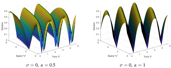
Figure 1.
Three-dimensional plots of Equation (12).
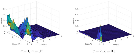
Figure 2.
Three-dimensional plots of Equation (12) with .
While in Figure 2 and Figure 3 below, we observe that after small transit patterns, the surface flattens significantly when noise is added and increased .
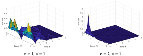
Figure 3.
Three-dimensional plots of Equation (12) with .
In Figure 4, we present a 2D graph of the u in (12) with and with , which emphasize the results above.
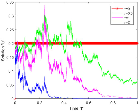
Figure 4.
Two-dimensional plots of Equation (12).
6. Conclusions
We presented a broad range of exact solutions to the stochastic fractional Kundu–Mukherjee–Naskar model (1). We applied two different methods, i.e., the Jacobi elliptic function method and the -expansion, to acquire elliptic, hyperbolic, trigonometric and rational stochastic fractional solutions. Such solutions are vital for appreciating some basically difficult complex phenomena. The obtained solutions will be highly beneficial for future investigations, such as ion-acoustic waves, oceanic rogue waves and optical fiber wave propagation in a magnetized plasma. Finally, the effect of noise on the analytical solution of the SFKMNE (1) is demonstrated. Since the multiplicative noise was addressed in this article, we may consider the additive noise in future work.
Author Contributions
Data curation, F.M.A.-A. and M.E.-M.; Formal analysis, W.W.M., F.M.A.-A. and C.C.; Funding acquisition, F.M.A.-A.; Methodology, C.C. and M.E.-M.; Project administration, W.W.M.; Software, W.W.M. and M.E.-M.; Supervision, C.C.; Visualization, F.M.A.-A.; Writing—original draft, M.E.-M.; Writing—review & editing, W.W.M. and C.C. All authors have read and agreed to the published version of the manuscript.
Funding
This research received no external funding.
Institutional Review Board Statement
Not applicable.
Informed Consent Statement
Not applicable.
Data Availability Statement
Not applicable.
Acknowledgments
Princess Nourah bint Abdulrahman University Researchers Supporting Project number (PNURSP2022R273), Princess Nourah bint Abdulrahman University, Riyadh, Saudi Arabia.
Conflicts of Interest
The authors declare no conflict of interest.
References
- Arnold, L. Random Dynamical Systems; Springer: Berlin/Heidelberg, Germany, 1998. [Google Scholar]
- Mohammed, W.W. Fast-diffusion limit for reaction–diffusion equations with degenerate multiplicative and additive noise. J. Dyn. Differ. Equ. 2021, 33, 577–592. [Google Scholar] [CrossRef]
- Imkeller, P.; Monahan, A.H. Conceptual stochastic climate models. Stoch. Dynam. 2002, 2, 311–326. [Google Scholar] [CrossRef]
- Iqbal, N.; Wu, R.; Mohammed, W.W. Pattern formation induced by fractional cross-diffusion in a 3-species food chain model with harvesting. Math. Comput. Simul. 2021, 188, 102–119. [Google Scholar] [CrossRef]
- Yan, Z.L. Abunbant families of Jacobi elliptic function solutions of the-dimensional integrable Davey-Stewartson-type equation via a new method. Chaos Solitons Fractals 2003, 18, 299–309. [Google Scholar] [CrossRef]
- Fan, E.; Zhang, J. Applications of the Jacobi elliptic function method to special-type nonlinear equations. Phys. Lett. A 2002, 305, 383–392. [Google Scholar] [CrossRef]
- Mohammed, W.W. Approximate solution of the Kuramoto-Shivashinsky equation on an unbounded domain. Chin. Ann. Math. Ser. B 2018, 39, 145–162. [Google Scholar] [CrossRef]
- Mohammed, W.W. Modulation Equation for the Stochastic Swift–Hohenberg Equation with Cubic and Quintic Nonlinearities on the Real Line. Mathematics 2020, 6, 1217. [Google Scholar] [CrossRef] [Green Version]
- Mohammed, W.W.; Iqbal, N. Impact of the same degenerate additive noise on a coupled system of fractional space diffusion equations. Fractals 2022, 30, 2240033. [Google Scholar] [CrossRef]
- Wazwaz, A.M. A sine-cosine method for handling nonlinear wave equations. Math. Comput. Model. 2004, 40, 499–508. [Google Scholar] [CrossRef]
- Yan, C. A simple transformation for nonlinear waves. Phys. Lett. A 1996, 224, 77–84. [Google Scholar] [CrossRef]
- Hirota, R. Exact solution of the Korteweg-de Vries equation for multiple collisions of solitons. Phys. Rev. Lett. 1971, 27, 1192–1194. [Google Scholar] [CrossRef]
- Wang, M.L.; Li, X.Z.; Zhang, J.L. The (G′G)-expansion method and travelling wave solutions of nonlinear evolution equations in mathematical physics. Phys. Lett. A 2008, 372, 417–423. [Google Scholar] [CrossRef]
- Zhang, H. New application of the (G′/G)-expansion method. Commun. Nonlinear Sci. Numer. Simul. 2009, 14, 3220–3225. [Google Scholar] [CrossRef]
- Mohammed, W.W.; Alesemi, M.; Albosaily, S.; Iqbal, N.; El-Morshedy, M. The exact solutions of stochastic fractional-space Kuramoto-Sivashinsky equation by using (G′/G)-expansion Method. Mathematics 2021, 9, 2712. [Google Scholar] [CrossRef]
- Khan, K.; Akbar, M.A. The exp(-φ(ς))-expansion method for finding travelling wave solutions of Vakhnenko-Parkes equation. Int. J. Dyn. Syst. Differ. Equ. 2014, 5, 72–83. [Google Scholar]
- Wazwaz, A.M. The tanh method: Exact solutions of the Sine–Gordon and Sinh–Gordon equations. Appl. Math. Comput. 2005, 167, 1196–1210. [Google Scholar] [CrossRef]
- Malfliet, W.; Hereman, W. The tanh method. I. Exact solutions of nonlinear evolution and wave equations. Phys. Scr. 1996, 54, 563–568. [Google Scholar] [CrossRef]
- Yang, X.F.; Deng, Z.C.; Wei, Y. A Riccati-Bernoulli sub-ODE method for nonlinear partial differential equations and its application. Adv. Differ. Equ. 2015, 1, 117–133. [Google Scholar] [CrossRef] [Green Version]
- Ma, W.-X.; Batwa, S. A binary darboux transformation for multicomponent NLS equations and their reductions. Anal. Math. Phys. 2021, 11, 44. [Google Scholar] [CrossRef]
- Khalil, R.; Al Horani, M.; Yousef, A.; Sababheh, M. A new definition of fractional derivative. J. Comput. Appl. Math. 2014, 264, 65–70. [Google Scholar] [CrossRef]
- Kundu, A.; Mukherjee, A. Novel integrable higher-dimensional nonlinear Schrödinger equation: Properties, solutions, applications. arXiv 2013, arXiv:1305.4023v1. [Google Scholar]
- Kundu, A.; Mukherjee, A.; Naskar, T. Modelling rogue waves through exact dynamical lump soliton controlled by ocean currents. Proc. R. Soc. A-Math. Phys. 2014, 470, 20130576. [Google Scholar] [CrossRef] [PubMed]
- Wen, X. Higher-order rational solutions for the (2+1)-dimensional KMN equation. Proc. Rom. Acad. A 2017, 18, 191–198. [Google Scholar]
- Mukherjee, A.; Kundu, A. Novel nonlinear wave equation: Regulated rogue waves and accelerated soliton solutions. Phys. Lett. A 2019, 383, 985–990. [Google Scholar] [CrossRef] [Green Version]
- Mukherjee, A.; Janaki, M.; Kundu, A. A new (2+1) dimensional integrable evolution equation for an ion acoustic wave in a magnetized plasma. Phys. Plasmas 2015, 22, 072302. [Google Scholar] [CrossRef] [Green Version]
- Ekici, M.; Sonmezoglu, A.; Biswas, A.; Belic, M.R. Optical solitons in (2+1)-Dimensions with Kundu-Mukherjee-Naskar equation by extended trial function scheme. Chin. J. Phys. 2019, 57, 72–77. [Google Scholar] [CrossRef]
- Yıldırım, Y. Optical solitons to Kundu-Mukherjee-Naskar model with trial equation approach. Optik 2019, 183, 1061–1065. [Google Scholar] [CrossRef]
- Yıldırım, Y. Optical solitons to Kundu-Mukherjee-Naskar model with modified simple equation approach. Optik 2019, 184, 247–252. [Google Scholar] [CrossRef]
- Kudryashov, N.A. General solution of traveling wave reduction for the Kundu–Mukherjee–Naskar model. Optik 2019, 186, 22–27. [Google Scholar] [CrossRef]
- Biswas, A.; Vega-Guzman, J.; Bansal, A.; Kara, A.H.; Biswas, A.; Vega-Guzman, J.; Bansal, A.; Kara, A.H.; Alzahrani, A.K.; Zhou, Q.; et al. Optical dromions, domain walls and conservation laws with Kundu-Mukherjee-Naskar equation via traveling waves and Lie symmetry. Results Phys. 2020, 16, 102850. [Google Scholar] [CrossRef]
- Mijena, J.B.; Nane, E. Space-time fractional stochastic partial differential equations. Stoch. Process. Appl. 2015, 125, 3301–3326. [Google Scholar] [CrossRef]
- Baeumer, B.; Geissert, M.; Kovacs, M. Existence, uniqueness and regularity for a class of semilinear stochastic Volterra equations with multiplicative noise. J. Differ. Equ. 2015, 258, 535–554. [Google Scholar] [CrossRef] [Green Version]
- Kloeden, P.E.; Platen, E. Numerical Solution of Stochastic Differential Equations; Springer: New York, NY, USA, 1995. [Google Scholar]
- Higham, D.J. An Algorithmic Introduction to Numerical Simulation of Stochastic Differential Equations. SIAM Rev. 2001, 43, 525–546. [Google Scholar] [CrossRef]
Publisher’s Note: MDPI stays neutral with regard to jurisdictional claims in published maps and institutional affiliations. |
© 2022 by the authors. Licensee MDPI, Basel, Switzerland. This article is an open access article distributed under the terms and conditions of the Creative Commons Attribution (CC BY) license (https://creativecommons.org/licenses/by/4.0/).