An Enriched Finite Element Method with Appropriate Interpolation Cover Functions for Transient Wave Propagation Dynamic Problems

Abstract

A novel enriched finite element method (EFEM) was employed to analyze the transient wave propagation problems. In the present method, the traditional finite element approximation was enriched by employing the appropriate interpolation covers. We mathematically and numerically showed that the present EFEM possessed the important monotonic convergence property with the decrease of the used time steps for transient wave propagation problems when the unconditional stable Newmark time integration scheme was used for time integration. This attractive property markedly distinguishes the present EFEM from the traditional FEM for transient wave propagation problems. Two typical numerical examples were given to demonstrate the capabilities of the present method.

1. Introduction

As is known to all, the transient wave propagation problems are usually encountered in many engineering application fields, such as aerospace and automotive industries, mechanical engineering, civil engineering and so on. During the past few decades, many numerical techniques have been developed that can be used to solve the wave propagation problems, such as the finite element method (FEM) [1], boundary element or boundary-type numerical techniques [2,3,4,5,6,7,8,9,10,11,12], finite difference method [13,14,15], smoothed FEM [16,17,18,19], collocation techniques [20,21,22] and various meshless methods [23,24,25,26,27,28,29,30,31,32,33,34]. Among them, the classical FEM is one of the most powerful and widely used numerical approaches for transient wave propagation analysis due to its rigorous mathematical background and good numerical stability [1].

However, the conventional FE solutions for transient wave propagation problems always suffer from the numerical dispersion issue induced by the spatial discretization and temporal discretization [35,36,37,38,39]. The former is related to the spatial interpolation and the used mesh, and the latter is mainly dominated by the used temporal discretization scheme. As a result, the obtained numerical waves are always dispersive and inaccurate. Another important point is that the quality of the FE solutions for transient wave propagation analysis cannot be improved constantly by using the decreasing temporal discretization steps for a fixed mesh pattern [40,41,42,43]. In other words, the time step for temporal discretization should be carefully determined according to the used mesh and the considered wave speed. Note that many different wave components with different speeds are always involved in transient wave propagation problems; so in general, these different wave components cannot be solved simultaneously with good computation accuracy. To address the drawbacks of the standard FEM in solving the transient wave propagation problems, the relatively new numerical techniques have still received quite considerable research efforts in the computational mechanics field. This is also the main motivation of the present work.

In this paper, we mainly focus on employing a novel enriched finite element method (EFEM) to analyze the transient wave propagation problems. In the present EFEM, the constructed interpolation covers are used to enrich the original FE approximation to improve the performance of the standard FEM in transient wave propagation analysis. We show in detail that the monotonic convergence property with the decrescent temporal discretization steps can be achieved for transient wave propagation problems. In consequence, all different types of waves with different propagation speeds can be simulated accurately as long as the temporal discretization steps for time integration are small enough. We provide two typical numerical examples to examine and investigate the capacities of the present EFEM in a transient wave propagation analysis.

The main structure of the present paper is as follows: Section 2.1 gives the problem statement of this work. In Section 2.2, the formulation of the EFEM for the transient wave propagation problem is given. A complete dispersion analysis is performed for the EFEM in Section 2.3. In the following section, the performance of the EFEM in solving the transient wave propagation problem is evaluated by the typical numerical examples. Section 4 gives our conclusions.

2. Formulation of the Present EFEM

2.1. Problem Statement

Consider a deformable elastic body occupying a bounded domain $V$. Assume that this elastic body is made of a homogeneous isotropic media and is subjected to a stress tensor $\tau \left(x,t\right)$ and body force vector $f_b\left(x,t\right)$. Based on the small displacement assumption, the strong from of this problem can be obtained as follows [1]

$$\rho \ddot{u}\left(x,t\right)=f_b\left(x,t\right)+\tau \left(x,t\right)n,$$

(1)

in which $u$ stands for the displacement, and $\rho$ represents the mass density of the linear elastic media; $\ddot{u}$ signifies two time derivatives.

By multiplying Equation (1) with a virtual displacement vector $\overline{u}$ and integrating by parts over the entire domain, we can obtain the following standard weak form of Equation (1)

$${\displaystyle {\int }_V{\overline{\mathsf{\epsilon }}}^T\mathsf{\tau }\mathrm{d}V+{\displaystyle {\int }_V\rho }}{\overline{u}}^T\ddot{u}\mathrm{d}V={\displaystyle {\int }_{s_f}{\overline{u}}^T{f}_{s_f}}\mathrm{d}S+{\displaystyle {\int }_V{\overline{u}}^T{f}_b}\mathrm{d}V,$$

(2)

in which $\overline{\mathsf{\epsilon }}$ denotes the virtual strain, and $f_{s_f}=\mathsf{\tau }\cdot n$ is the imposed boundary traction vector.

Using the standard finite element formulation, we can obtain the following matrix form of Equation (2)

$$M\ddot{u}\left(t\right)+C\dot{u}\left(t\right)+Ku\left(t\right)=F\left(t\right),$$

(3)

in which $F\left(t\right)$ is the applied force vector, $K$ is the stiffness matrix, $M$ is the mass matrix and $C$ is a matrix corresponding to the damping effects.

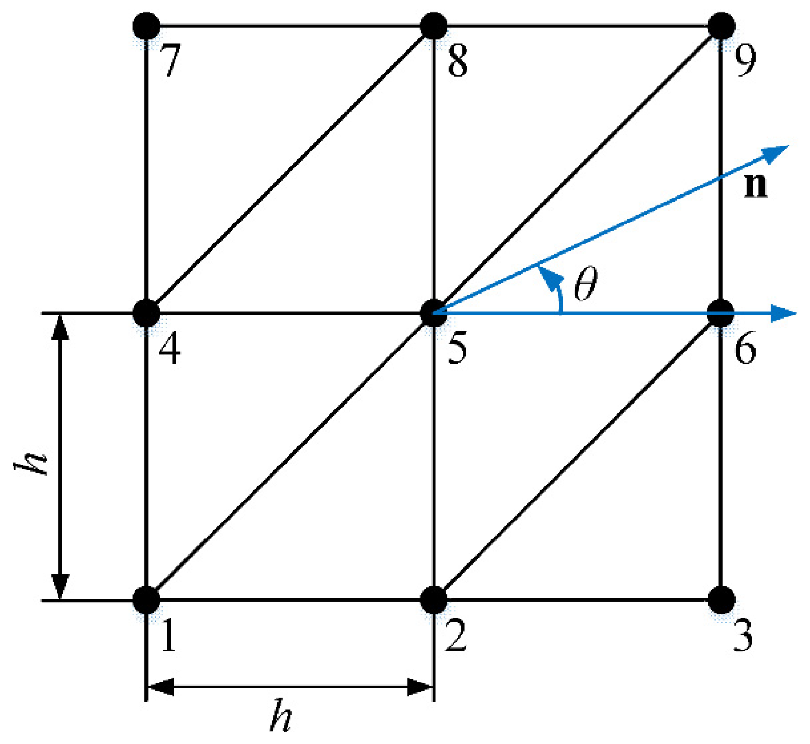
2.2. Formulation of the EFEM

In the enriched finite element model, the standard finite element interpolation for the considered field variable u at node i is enriched by the following expression [37,41]

$$E_i^q\left[u\right]=L{\left[\begin{array}{ccccc}{u}_i& a_{i1}& a_{i2}& a_{i3}& \cdots \end{array}\right]}^T,$$

(4)

in which ${\left[\begin{array}{cccc}{a}_{i1}& a_{i2}& a_{i3}& \cdots \end{array}\right]}^T$ denotes the additional unknown coefficients, and $u_i$ stands for the conventional nodal displacement corresponding to node i; $L$ denotes the local interpolation basis functions.

For the two-dimensional problems, which are discretized into regular mesh with average nodal space h, the following linear polynomials and trigonometric functions are always used as the local interpolation basis functions [35]

$$L=\left\{\begin{array}{l}\begin{array}{cccc}1,& {\overline{x}}_i,& {\overline{y}}_i,& {\overline{x}}_i{\overline{y}}_i\end{array}\\ \begin{array}{cccc}\cos \left(\frac{2\mathsf{\pi }{\overline{x}}_i}{{\lambda }_x}\right),& \sin \left(\frac{2\mathsf{\pi }{\overline{x}}_i}{{\lambda }_x}\right),& \cos \left(\frac{2\mathsf{\pi }{\overline{y}}_i}{{\lambda }_y}\right),& \sin \left(\frac{2\mathsf{\pi }{\overline{y}}_i}{{\lambda }_y}\right),\end{array}\\ \begin{array}{cccc}\cos \left(\frac{2\mathsf{\pi }{\overline{x}}_i}{{\lambda }_x}+\frac{2\mathsf{\pi }{\overline{y}}_i}{{\lambda }_y}\right),& \sin \left(\frac{2\mathsf{\pi }{\overline{x}}_i}{{\lambda }_x}+\frac{2\mathsf{\pi }{\overline{y}}_i}{{\lambda }_y}\right),& \cos \left(\frac{2\mathsf{\pi }{\overline{x}}_i}{{\lambda }_x}-\frac{2\mathsf{\pi }{\overline{y}}_i}{{\lambda }_y}\right),& \sin \left(\frac{2\mathsf{\pi }{\overline{x}}_i}{{\lambda }_x}-\frac{2\mathsf{\pi }{\overline{y}}_i}{{\lambda }_y}\right),\end{array}\\ \begin{array}{ccc}& \cdots ,& \end{array}\\ \begin{array}{cccc}\cos \left(\frac{2\mathsf{\pi }q{\overline{x}}_i}{{\lambda }_x}\right),& \sin \left(\frac{2\mathsf{\pi }q{\overline{x}}_i}{{\lambda }_x}\right),& \cos \left(\frac{2\mathsf{\pi }q{\overline{y}}_i}{{\lambda }_y}\right),& \sin \left(\frac{2\mathsf{\pi }q{\overline{y}}_i}{{\lambda }_y}\right),\end{array}\\ \begin{array}{cccc}\cos \left(\frac{2\mathsf{\pi }q{\overline{x}}_i}{{\lambda }_x}+\frac{2\mathsf{\pi }q{\overline{y}}_i}{{\lambda }_y}\right),& \sin \left(\frac{2\mathsf{\pi }q{\overline{x}}_i}{{\lambda }_x}+\frac{2\mathsf{\pi }q{\overline{y}}_i}{{\lambda }_y}\right),& \cos \left(\frac{2\mathsf{\pi }q{\overline{x}}_i}{{\lambda }_x}-\frac{2\mathsf{\pi }q{\overline{y}}_i}{{\lambda }_y}\right),& \sin \left(\frac{2\mathsf{\pi }q{\overline{x}}_i}{{\lambda }_x}-\frac{2\mathsf{\pi }q{\overline{y}}_i}{{\lambda }_y}\right)\end{array}\end{array}\right\}$$

(5)

in which the relative coordinate values $\left({\overline{x}}_i,{\overline{y}}_i\right)$ are measured from node i, namely ${\overline{x}}_i=x-x_i$ and ${\overline{y}}_i=y-y_i$; the used trigonometric function is of q order; in this work, $q=1$ and ${\lambda }_x={\lambda }_y=2h$ are employed. Although the higher order of polynomials and trigonometric functions also can be used to construct the local enrichment functions, the involved numerical integration is accordingly more numerically expensive.

Then Equation (4) can also be written by [37,41]

$$E_i^q\left[u\right]=u_i+\underset{\mathrm{additional}\mathrm{interpolation}\mathrm{cover}}{\underbrace{\left[\begin{array}{ccccccc}{\overline{x}}_i& {\overline{y}}_i& {\overline{x}}_i{\overline{y}}_i& \cos \left(\frac{2\mathsf{\pi }{\overline{x}}_i}{{\lambda }_x}\right)& \sin \left(\frac{2\mathsf{\pi }{\overline{x}}_i}{{\lambda }_x}\right)& \cdots & \sin \left(\frac{2\mathsf{\pi }{\overline{x}}_i}{{\lambda }_x}-\frac{2\mathsf{\pi }{\overline{y}}_i}{{\lambda }_y}\right)\end{array}\right]\left[\begin{array}{c}{a}_{i1}\\ a_{i2}\\ ⋮\\ a_{i10}\end{array}\right]}},$$

(6)

From Equation (6), the distinct difference between the traditional FE approximation and the present enriched FE approximation can be seen because the present EFEM contains the additional interpolation cover in the interpolation scheme.

When the standard linear triangular element with the usual linear interpolation function N_i is used, the global displacement u can be expressed by [37]

$$T{E}_i^q\left[u\right]={\displaystyle \sum _1^m\left({\displaystyle \sum _{i=1}^3{N}_i{E}_i^q\left[u\right]}\right)}={\displaystyle \sum _1^m\left({\displaystyle \sum _{i=1}^3{N}_i{u}_i+{\displaystyle \sum _{i=1}^3{H}_i{a}_i}}\right)}={\displaystyle \sum _1^m\left({\displaystyle \sum _{i=1}^3{N}_i{u}_i+{\displaystyle \sum _{i=1}^3{\displaystyle \sum _{j=1}^n{H}_{i,j}{a}_{i,j}}}}\right)},$$

(7)

in which j is the additional degree of freedom for node i, and m is the total number of nodes in the problem domain.

$$H_i=N_i\left[\begin{array}{ccccccc}{\overline{x}}_i& {\overline{y}}_i& {\overline{x}}_i{\overline{y}}_i& \cos \left(\frac{2\mathsf{\pi }{\overline{x}}_i}{{\lambda }_x}\right)& \sin \left(\frac{2\mathsf{\pi }{\overline{x}}_i}{{\lambda }_x}\right)& \cdots & \sin \left(\frac{2\mathsf{\pi }{\overline{x}}_i}{{\lambda }_x}-\frac{2\mathsf{\pi }{\overline{y}}_i}{{\lambda }_y}\right)\end{array}\right],$$

(8)

From Equations (6) and (7), it is seen that when we only use the constant term 1 in Equation (5) as the local enrichment function for required interpolation, the present EFEM will become the standard FEM. Therefore, the proposed EFEM in this work is actually the combination of the higher interpolation and the conventional FE interpolation. Using the present EFEM, the computation accuracy of the obtained numerical solutions can be markedly increased without adding the additional nodes, because the higher interpolation can be obtained using the low-order linear elements.

2.3. Dispersion Analysis

When the FEM-like numerical techniques are used for wave analysis, the involved numerical dispersion error issue should be carefully addressed because it is able to strongly influence the computation accuracy of the obtained numerical solutions. Therefore, the dispersion properties of the present EFEM will be evaluated carefully in this sub-section. As shown in Figure 1, in the dispersion analysis, the uniform triangular mesh is used, the blue line denotes the wave propagation direction $\theta$ and h stands for the average mesh size of the used mesh.

By eliminating the time dependency from Equation (3) and without considering the boundary conditions, we have [35,37]

$$\left(\mathbf{K}-k^2\mathbf{M}\right)a=0,$$

(9)

in which $a={\left[\begin{array}{ccccc}{u}_i& a_{i1}& a_{i2}& a_{i3}& \cdots \end{array}\right]}^T$ lists all unknown solution coefficients, and $k$ is the wave number.

Using the enriched finite element interpolation scheme shown in Equation (7) and referring to the uniform mesh shown in Figure 1, for one typical node, we can obtain [35,37]

$$[{\mathbf{D}}_{\mathrm{stiff}}-k^2{\mathrm{D}}_{\mathrm{mass}}]a_i=0,$$

(10)

in which ${\mathbf{D}}_{\mathrm{stiff}}$ and ${\mathbf{D}}_{\mathrm{mass}}$ are the obtained Hermitian matrices of order $n_p\times n_p$, corresponding to the stiffness matrix $\mathbf{K}$ and mass matrix $\mathbf{M}$; $n_p$ is the total number of unknown solution coefficients for each node and $a_i={\left[\begin{array}{cccc}{A}_1& A_2& \cdots & A_{n_p}\end{array}\right]}^T$ is the amplitude vector for one typical node i [35,37].

If the nontrivial solutions to Equation (10) exist, we must have [35,37]

$$\det [{\mathbf{D}}_{\mathrm{stiff}}-k^2{\mathbf{D}}_{\mathrm{mass}}]=0,$$

(11)

Note that the numerical wave number $k_h$ is involved in the matrices ${\mathbf{D}}_{\mathrm{stiff}}$ and ${\mathbf{D}}_{\mathrm{mass}}$ [35,37]; hence, the corresponding exact wave number $k$ can be calculated using Equation (11) for any given $k_h$. Owing to the numerical dispersion issue by the spatial discretization, $k$ is in general different from $k_h$. In this work, the obtained spatial dispersion error by the numerical methods is quantified by using the measure $k/k_h$.

Figure 2 shows the calculated spatial dispersion error $k/k_h$ from the standard FEM and the present EFEM as a function of the non-dimensional wave number $kh$ along different wave propagation directions. It is seen that the spatial dispersion error from FEM is much larger than that from the present EFEM for the considered non-dimensional wave number.

The numerical dispersion error from the temporal discretization is also investigated in this section. Here, the additional boundary conditions and the damping effects are not considered. Assuming that all the variables in Equation (3) are time-harmonic, then the following matrix equation can be arrived at [35,37]

$$M\ddot{\overline{a}}+c^{2}K\overline{a}=0,$$

(12)

in which $c$ is the wave speed, $\overline{a}=\widehat{a}{e}^{j\left(k_{h}n\cdot x-{\omega }_{h}t\right)}$ and ${\omega }_h$ is the numerical angular frequency.

Using the Newmark time integration method with the parameters $\delta =1/2$ and $\alpha =1/4$ for temporal discretization, we can obtain the following discretized equation [1]

$$(M+\frac{1}{4}{\omega }^2\Delta t^{2}K{)}^{t+\Delta t}U+(-2M+\frac{1}{2}{\omega }^2\Delta t^{2}K{)}^{t}U+(M+\frac{1}{4}{\omega }^2\Delta t^{2}K{)}^{t-\Delta t}U=0,$$

(13)

in which $\Delta t$ is the used temporal discretization step, and $\omega$ is the exact angular frequency.

Based on the formulation in Ref. [35], the following equation can be arrived at

$${\omega }_h\Delta t=j\ln \left(\frac{-m\pm \sqrt{m^2-4nl}}{2l}\right),$$

(14)

in which $l=1+\frac{1}{4}{\omega }^2\Delta t^2$, $m=-2+\frac{1}{2}{\omega }^2\Delta t^2$ and $n=1+\frac{1}{4}{\omega }^2\Delta t^2$.

In Equation (14) we can see that the right side of the equation only contains the parameter $\omega \Delta t$; hence, the parameter ${\omega }_h\Delta t$ is actually a function of the parameter $\omega \Delta t$, namely

$${\omega }_h\Delta t=f\left(\omega \Delta t\right)=f\left(kh\frac{c\Delta t}{h}\right)=f\left(kh\mathrm{CFL}\right),$$

(15)

where CFL = $c\Delta t/h$ is the defined Courant–Friedrichs–Lewy (CFL) number [35,37].

Then, for transient wave propagations, the total numerical dispersion error can be calculated using the following equation

$$\frac{c_h}{c}=\frac{{\omega }_h/k_h}{c}=\frac{{\omega }_h\Delta t}{k_{h}c\Delta t}=\frac{{\omega }_h\Delta t}{k_{h}h\mathrm{CFL}}=\frac{f\left(\omega \Delta t\right)}{k_{h}h\mathrm{CFL}}=\frac{f\left(kh\mathrm{CFL}\right)}{k_{h}h\mathrm{CFL}},$$

(16)

Using the Taylor series expansion, we have

$$\begin{array}{ll}\frac{c_h}{c}& =\frac{1}{k_{h}h\mathrm{CFL}}\left[\underset{=0}{\underbrace{f\left(0\right)}}+f^{\prime }\left(0\right)\left(kh\mathrm{CFL}\right)+\frac{1}{2!}\underset{=0}{\underbrace{f^{″}\left(0\right)}}{\left(kh\mathrm{CFL}\right)}^2+\frac{1}{3!}{f}^{\left(3\right)}\left(0\right){\left(kh\mathrm{CFL}\right)}^3+\cdots \right]\\ & =\frac{k}{k_h}\underset{\mathrm{Temporal}\mathrm{dispersion}\mathrm{error}}{\underbrace{\left(1-\frac{1}{12}{\left(kh\mathrm{CFL}\right)}^2+\frac{1}{80}{\left(kh\mathrm{CFL}\right)}^4+\cdots \right)}}\end{array}$$

(17)

Note that $\frac{c_h}{c}=\frac{{\omega }_h/k_h}{\omega /k}=\frac{k}{k_h}\frac{{\omega }_h}{\omega }=\frac{k}{k_h}\frac{T}{T_h}$, in which $T$ and $T_h$ are, respectively, the exact and numerical period of the wave mode; then, we can have

$$\frac{c_h}{c}=\frac{k}{k_h}\frac{T}{T_h}=\frac{k}{k_h}\underset{\mathrm{Temporal}\mathrm{dispersion}\mathrm{error}}{\underbrace{\left(1-\frac{1}{12}{\left(kh\mathrm{CFL}\right)}^2+\frac{1}{80}{\left(kh\mathrm{CFL}\right)}^4+\cdots \right)}},$$

(18)

From above formulation, we can obtain the following important observations:

(1) The total dispersion error $c_h/c$ for transient wave analysis clearly contains two different parts, namely $k/k_h$ and $T/T_h$, which are respectively caused by the spatial discretization method (FEM and the present EFEM) and the time integration scheme for temporal discretization.

(2) $T/T_h$ is basically a monotonic function with respect to sufficiently small CFL numbers when the spatial discretization step h and the considered wave number k are determined. In other words, $T/T_h$ will approach 1 when the temporal discretization step $\Delta t$, which is related to the CFL number, gets smaller, namely $T/T_h\to 1$ can be obtained when $\Delta t\to 0$.

(3) Both the spatial and temporal discretization are able to affect the total dispersion error $c_h/c$. The effects from these two different factors can be counteracted to some degree, because in general, $T/T_h<1$ and $k/k_h>1$. In addition, we also can observe that $c_h/c$ will tend to $k/k_h$ when $\Delta t\to 0$ (namely $\mathrm{CFL}\to 0$), because $T/T_h\to 1$ can be obtained when $\Delta t\to 0$.

(4) There exists an optimal time step $\Delta t$ (namely the optimal CFL_opt) which can lead to almost non-dispersive numerical solutions, namely $c_h/c\approx 1$.

Based on the above findings, we can see that for transient wave analysis, the obtained total dispersion error $c_h/c$ from the proposed EFEM and the Newmark time integration scheme can be basically decreased by using the decreasing temporal discretization step $\Delta t$. As a result, the obtained numerical solutions from the EFEM and Newmark method will approach the “exact” solutions when the temporal discretization step $\Delta t$ tends to zero, because the involved spatial dispersion error $k/k_h$ is very small for $kh<\mathsf{\pi }$ (see Figure 2); hence, the so-called monotonic convergence property with respect to the temporal discretization step $\Delta t$ can be reached, while this important and attractive property is not applicable for the standard FEM because the resultant spatial discretization error from the standard FEM is much larger than that from the EFEM (see Figure 2).

In addition, it should be noted that the involved linear dependence (LD) problem should be carefully addressed when the EFEM is employed for engineering computation. Owing to the LD problem, the nearly singular matrix equation can always be obtained, especially as the used local enrichment functions are constructed by the polynomials. In [37], the LD issue of the EFEM was investigated systematically, and the LD could be totally suppressed by an elegantly-designed scheme. Using this scheme, the relatively high computation accuracy of the EFEM could be completely maintained by removing the sufficiently few cover degrees of freedom (DOFs). In this work, the LD problem of the EFEM is addressed by using the scheme proposed in [37], and the performance of the EFEM for complicated transient waves is examined.

3. Numerical Example

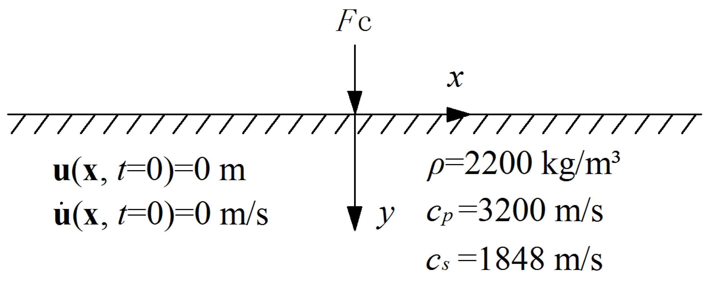
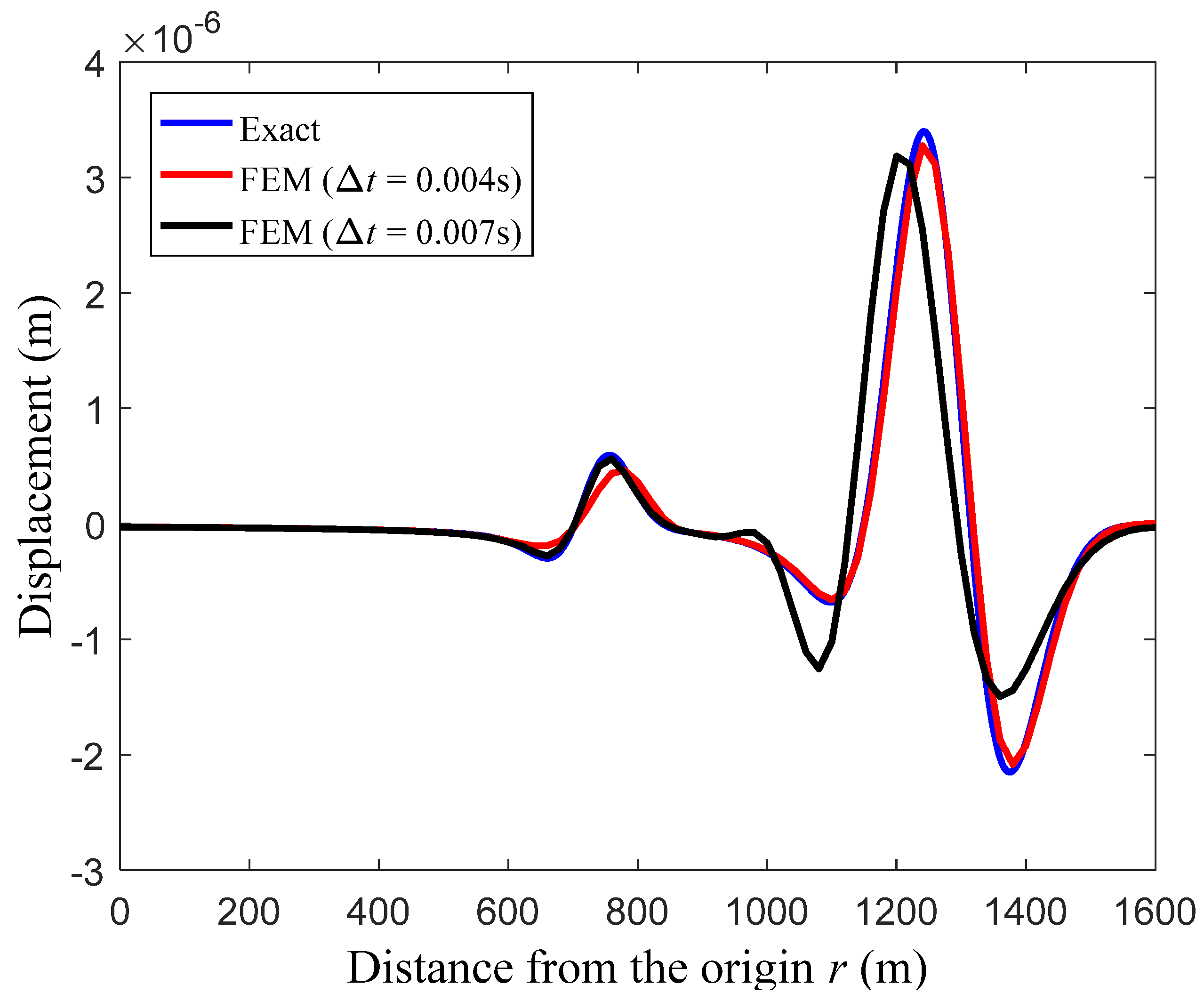
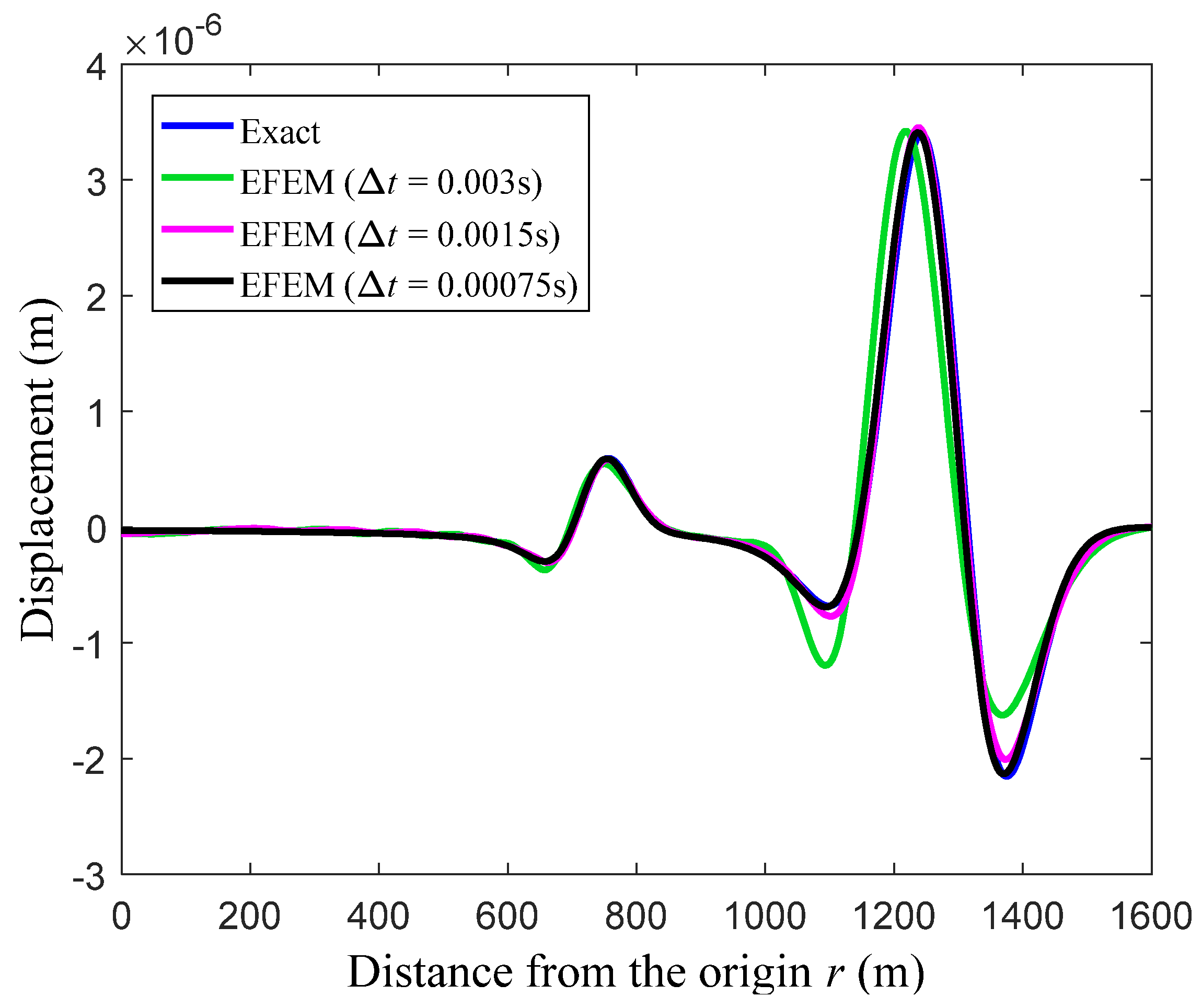
3.1. The Lamb’s Problem

In this sub-section, the hardware configuration of the used laptop were two cores Intel 2.50 GHz CPU and 4 GB RAM. Firstly, the well-known Lamb’s problem, with plane strain conditions in which the two-dimensional elastic wave propagations are involved, has been considered to investigate the capabilities of the present EFEM in transient wave propagation analysis. As shown in Figure 3, the material parameters of the considered elastic medium are mass density $\rho =$2200 kg/m³, P-wave velocity c_p = 3200 m/s and S-wave velocity c_s = 1848 m/s. The uniform triangular mesh with nodal space h = 20 m ias employed in the calculation. The following concentrated line load [37] is imposed at the free surface of the elastic medium.

$$F_c=2\times {10}^6\left[1-2{\mathsf{\pi }}^2{f}_p^2{\left(t-t_s\right)}^2\right]\exp \left[-{\mathsf{\pi }}^2{f}_p^2{\left(t-t_s\right)}^2\right],$$

(19)

where $f_p$ = 10 Hz is the peak frequency, and $t_s=$0.1 s is the time shift.

Figure 4 gives the calculated displacement solutions from the standard FEM along the y-axis at the observation time t = 0.5 s; the higher and lower peaks correspond to the P-wave and S-wave, respectively. From the discussion in Section 2, it is known that the conventional FEM does not have the monotonic convergence property with the decreasing temporal discretization step; however, there exists an optimal time step (which is related to the crucial parameter CFL) for each wave component. Using the optimal time step, the minimal numerical dispersion error can be obtained [1]. In Figure 4, two different time steps $\Delta t$ = 0.004 s and $\Delta t$ = 0.007 s are used for time integration; these two time steps approximately correspond to the optimal CFL = 0.65 [40] for the P-wave and S-wave, respectively. From Figure 4, it is clearly seen that the P-wave and S-wave can be accurately simulated using the corresponding optimal steps; however, these two different elastic wave components with different speeds cannot be predicted simultaneously with sufficiently good accuracy.

Figure 5 presents the corresponding numerical solutions from the present EFEM using three time steps for time integration. It is seen that both the P-wave and S-wave solutions will converge monotonically to the exact solutions with the decrease of the temporal discretization step. The reason for this is that the so-called monotonic convergence property can be basically reached when the transient wave propagations are analyzed by the EFEM, so all considered wave components with different speeds can be accurately solved as long as the used time step is small enough. In addition, the von Mises stress distribution results from the present EFEM are also calculated and shown in Figure 6; we can see that the physical behaviors of all different wave components can be accurately simulated. From these numerical results, we can see that the proposed EFEM possesses very excellent properties and is a powerful numerical approach to tackle the transient wave propagations.

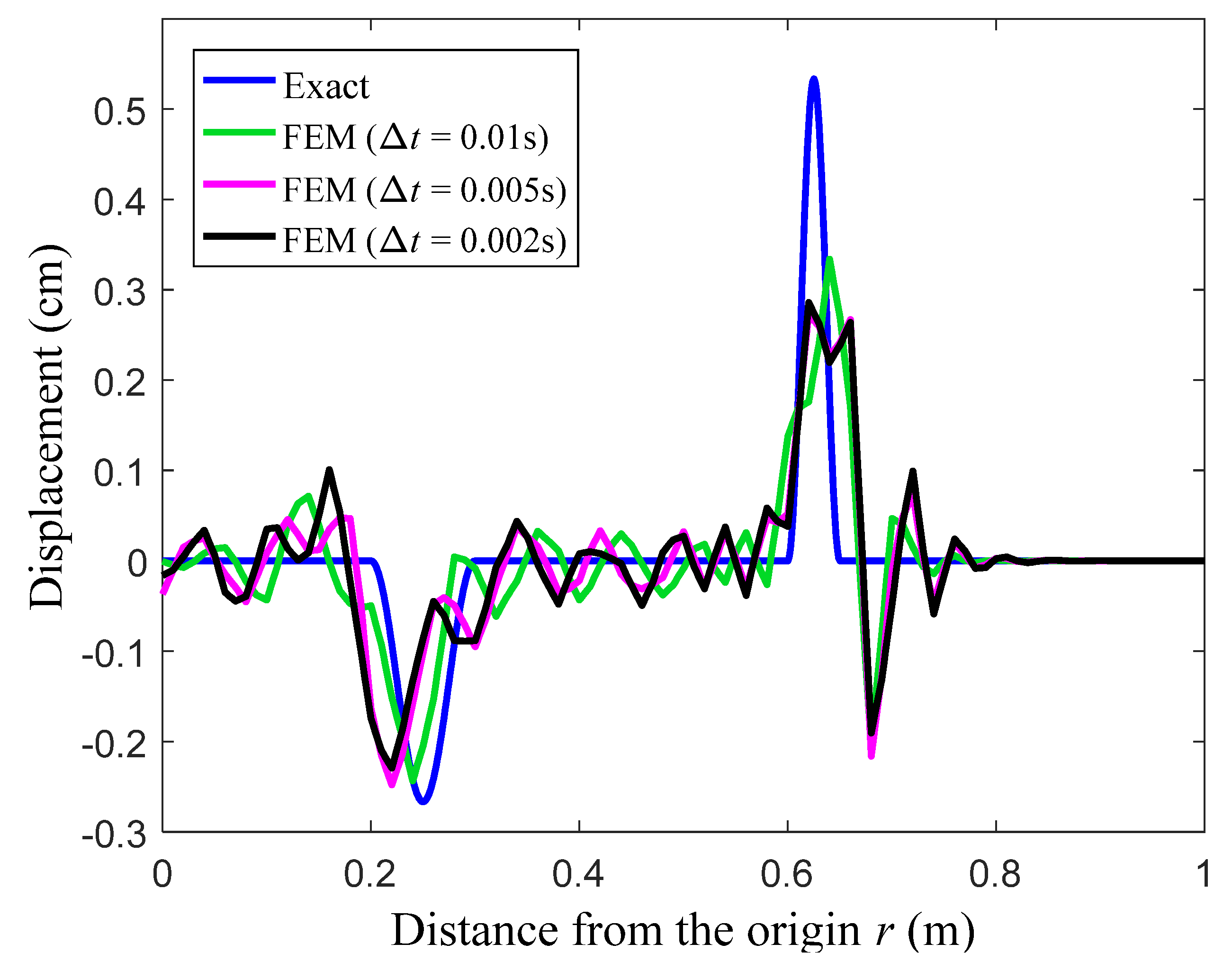
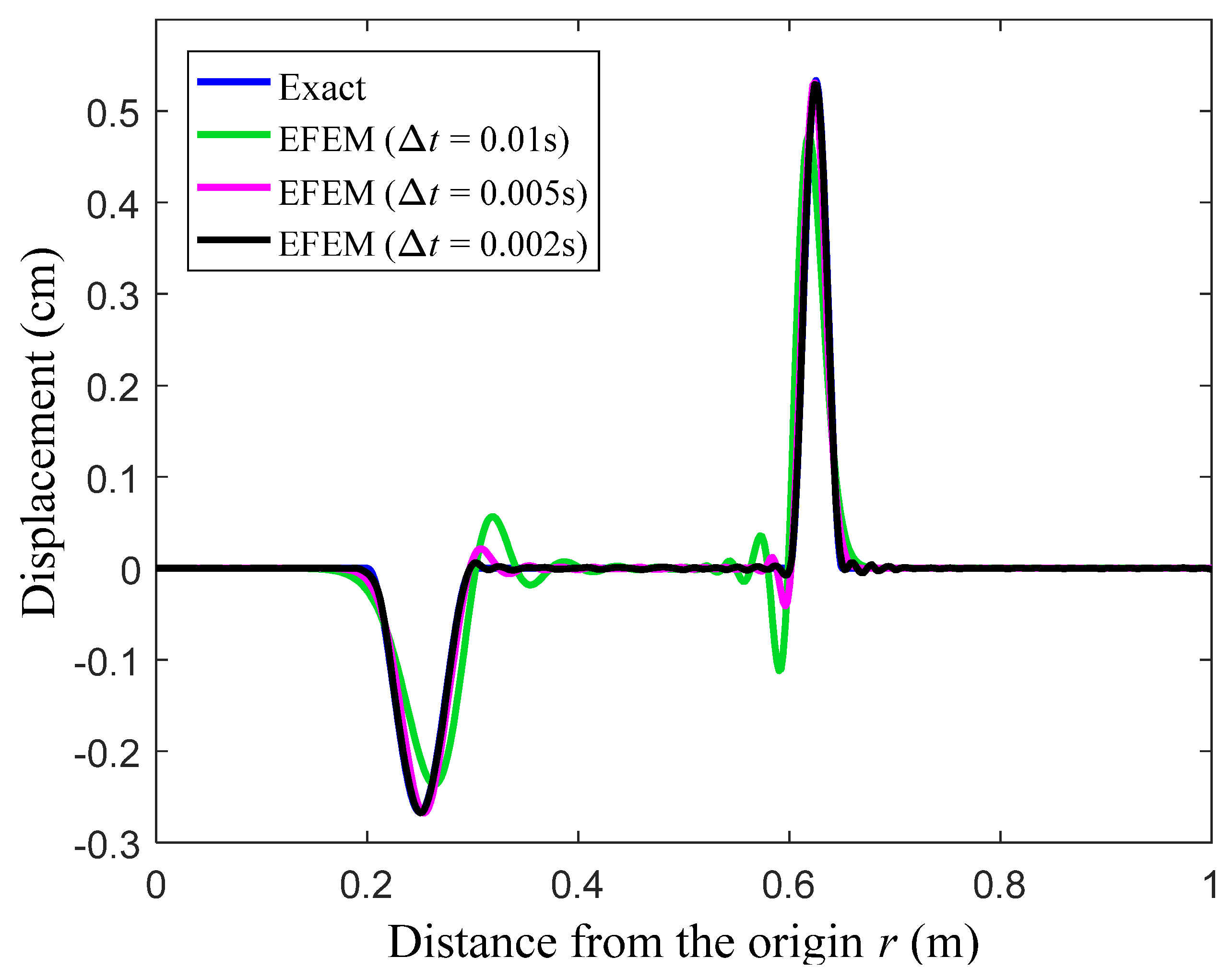
3.2. The Transient Wave Propagation along an Elastic Bar

In this sub-section, we further examine the abilities of the EFEM by studying the scalar wave propagation along a one-dimensional elastic bar. As shown in Figure 7, the right end of the bar is fixed, and the elastic bar is made of two different elastic media (which are represented in blue and black lines) with wave propagation speed c₁ = 1 m/s and c₂ = 2 m/s. The problem domain is discretized into a uniform mesh with nodal space h = 0.02 m. Assuming that a sinusoidal wave $u=0.8\sin \left(20\mathsf{\pi }t\right)\mathrm{cm}$, $t\in \left[\begin{array}{cc}0,& 0.05\end{array}\right]\mathrm{s}$ begins to travel along this bar from the left end.

At the observation time t = 0.8 s, the displacement solutions from the standard FEM with linear elements and the present EFEM with linear polynomials and trigonometric enrichment functions are given in Figure 8 and Figure 9. It is known that both reflected and transmitted waves will be induced in this problem, and it is easily to identify that in the figures, the small and large peaks, respectively, correspond to reflected and transmitted wave components. Similar to the previous numerical example, several different time steps are used in the calculation. From the results in Figure 8 and Figure 9, the similar observations, which have been found in the previous numerical example, can again be obtained, namely all different wave components with different wave propagation speeds can be accurately predicted using the present EFEM when the used time step gets smaller, while the different waves cannot be predicted simultaneously in sufficiently good accuracy by the standard FEM.

4. Conclusions

In this work, a novel enriched finite element method (EFEM) with additional appropriate interpolation cover functions was developed for transient wave propagation analysis. In the present EFEM, the additional linear polynomials and trigonometric functions were used to enrich the original nodal shape functions of the traditional FEM. It was mathematically and numerically shown that the present EFEM possessed the important and attractive monotonic convergence property with the decreasing temporal discretization steps in solving transient wave propagation problems; so, all different wave components with different propagation speeds could be accurately predicted using the sufficiently small time step. Therefore, the present EFEM is also a prospective powerful approach to deal with the elastic wave propagation in anisotropic media and multiple waves propagation in laminated composite structures.

References

1. Bathe, K.J. Finite Element Procedures, 2nd ed.; Prentice Hall: Watertown, MA, USA, 2014. [Google Scholar]
2. Li, J.P.; Gu, Y.; Qin, Q.H.; Zhang, L. The rapid assessment for three-dimensional potential model of large-scale particle system by a modified multilevel fast multipole algorithm. Comput. Math. Appl. 2021, 89, 127–138. [Google Scholar] [CrossRef]
3. Gu, Y.; Lei, J. Fracture mechanics analysis of two-dimensional cracked thin structures (from micro- to nano-scales) by an efficient boundary element analysis. Results Math. 2021, 11, 100172. [Google Scholar] [CrossRef]
4. Gu, Y.; Fan, C.M.; Fu, Z.J. Localized method of fundamental solutions for three-dimensional elasticity problems: Theory. Adv. Appl. Math. Mech. 2021, 13, 1520–1534. [Google Scholar]
5. Wang, F.; Fan, C.M.; Zhang, C.; Lin, J. A localized space-time method of fundamental solutions for diffusion and convection-diffusion problems. Adv. Appl. Math. Mech. 2020, 12, 940–958. [Google Scholar] [CrossRef]
6. Li, J.P.; Fu, Z.J.; Gu, Y.; Qin, Q.H. Recent advances and emerging applications of the singular boundary method for large-scale and high-frequency computational acoustics. Adv. Appl. Math. Mech. 2022, 14, 315–343. [Google Scholar] [CrossRef]
7. Liu, C.S.; Qiu, L.; Lin, J. Simulating thin plate bending problems by a family of two-parameter homogenization functions. Appl. Math. Model. 2020, 79, 284–299. [Google Scholar] [CrossRef]
8. Fu, Z.J.; Xi, Q.; Li, Y.; Huang, H.; Rabczuk, T. Hybrid FEM–SBM solver for structural vibration induced underwater acoustic radiation in shallow marine environment. Comput. Methods Appl. Mech. Eng. 2020, 369, 113236. [Google Scholar] [CrossRef]
9. Fu, Z.J.; Chen, W.; Wen, P.H.; Zhang, C.Z. Singular boundary method for wave propagation analysis in periodic structures. J. Sound Vib. 2018, 425, 170–188. [Google Scholar] [CrossRef]
10. Cheng, S.F.; Wang, F.J.; Wu, G.Z.; Zhang, C.X. Semi-analytical and boundary-type meshless method with adjoint variable formulation for acoustic design sensitivity analysis. Appl. Math. Lett. 2022, 131, 108068. [Google Scholar] [CrossRef]
11. Li, J.P.; Zhang, L. High-precision calculation of electromagnetic scattering by the Burton-Miller type regularized method of moments. Eng. Anal. Bound. Elem. 2021, 133, 177–184. [Google Scholar] [CrossRef]
12. Li, J.P.; Zhang, L.; Qin, Q.H. A regularized method of moments for three-dimensional time-harmonic electromagnetic scattering. Appl. Math. Lett. 2021, 112, 106746. [Google Scholar] [CrossRef]
13. Qu, W.Z.; He, H. A GFDM with supplementary nodes for thin elastic plate bending analysis under dynamic loading. Appl. Math. Lett. 2022, 124, 107664. [Google Scholar] [CrossRef]
14. Qu, W.Z.; Gao, H.W.; Gu, Y. Integrating Krylov deferred correction and generalized finite difference methods for dynamic simulations of wave propagation phenomena in long-time intervals. Adv. Appl. Math. Mech. 2021, 13, 1398–1417. [Google Scholar]
15. Fu, Z.J.; Xie, Z.Y.; Ji, S.Y.; Tsai, C.C.; Li, A.L. Meshless generalized finite difference method for water wave interactions with multiple-bottom-seated-cylinder-array structures. Ocean Eng. 2020, 195, 106736. [Google Scholar] [CrossRef]
16. Chai, Y.B.; Gong, Z.X.; Li, W.; Li, T.Y.; Zhang, Q.F.; Zou, Z.H.; Sun, Y.B. Application of smoothed finite element method to two dimensional exterior problems of acoustic radiation. Int. J. Comput. Methods 2018, 15, 1850029. [Google Scholar] [CrossRef]
17. Chai, Y.B.; You, X.Y.; Li, W.; Huang, Y.; Yue, Z.J.; Wang, M.S. Application of the edge-based gradient smoothing technique to acoustic radiation and acoustic scattering from rigid and elastic structures in two dimensions. Comput. Struct. 2018, 203, 43–58. [Google Scholar] [CrossRef]
18. Chai, Y.B.; Li, W.; Gong, Z.X.; Li, T.Y. Hybrid smoothed finite element method for two-dimensional underwater acoustic scattering problems. Ocean Eng. 2016, 116, 129–141. [Google Scholar] [CrossRef]
19. Li, W.; Gong, Z.X.; Chai, Y.B.; Cheng, C.; Li, T.Y.; Zhang, Q.F.; Wang, M.S. Hybrid gradient smoothing technique with discrete shear gap method for shell structures. Comput. Math. Appl. 2017, 74, 1826–1855. [Google Scholar] [CrossRef]
20. Wang, F.; Zhao, Q.; Chen, Z.; Fan, C.M. Localized Chebyshev collocation method for solving elliptic partial differential equations in arbitrary 2D domains. Appl. Math. Comput. 2021, 397, 125903. [Google Scholar] [CrossRef]
21. Xi, Q.; Fu, Z.J.; Zhang, C.Z.; Yin, D.S. An efficient localized Trefftz-based collocation scheme for heat conduction analysis in two kinds of heterogeneous materials under temperature loading. Comput. Struct. 2021, 255, 106619. [Google Scholar] [CrossRef]
22. Xi, Q.; Fu, Z.J.; Wu, W.J.; Wang, H.; Wang, Y. A novel localized collocation solver based on Trefftz basis for Potential-based Inverse Electromyography. Appl. Math. Comput. 2021, 390, 125604. [Google Scholar] [CrossRef]
23. Liu, G.R. Mesh Free Methods: Moving Beyond the Finite Element Method; CRC Press: Boca Raton, FL, USA, 2009. [Google Scholar]
24. Li, X.; Li, S. A fast element-free Galerkin method for the fractional diffusion-wave equation. App. Math. Lett. 2021, 122, 107529. [Google Scholar] [CrossRef]
25. Qiu, L.; Lin, J.; Wang, F.J.; Qin, Q.H.; Liu, C.S. A homogenization function method for inverse heat source problems in 3D functionally graded materials. Appl. Math. Model. 2021, 91, 923–933. [Google Scholar] [CrossRef]
26. You, X.Y.; Li, W.; Chai, Y.B. A truly meshfree method for solving acoustic problems using local weak form and radial basis functions. Appl. Math. Comput. 2020, 365, 124694. [Google Scholar] [CrossRef]
27. Lin, J.; Zhang, Y.H.; Reutskiy, S.; Feng, W. A novel meshless space-time backward substitution method and its application to nonhomogeneous advection-diffusion problems. Appl. Math. Comput. 2021, 398, 125964. [Google Scholar] [CrossRef]
28. Li, W.; Zhang, Q.; Gui, Q.; Chai, Y.B. A coupled FE-Meshfree triangular element for acoustic radiation problems. Int. J. Comput. Methods 2021, 18, 2041002. [Google Scholar] [CrossRef]
29. Li, X.; Li, S. A finite point method for the fractional cable equation using meshless smoothed gradients. Eng. Anal. Bound. Elem. 2022, 134, 453–465. [Google Scholar] [CrossRef]
30. Gu, Y.; Sun, H. A meshless method for solving three-dimensional time fractional diffusion equation with variable-order derivatives. Appl. Math. Model. 2020, 78, 539–549. [Google Scholar] [CrossRef]
31. Qu, J.; Dang, S.N.; Li, Y.C.; Chai, Y.B. Analysis of the interior acoustic wave propagation problems using the modified radial point interpolation method (M-RPIM). Eng. Anal. Bound. Elem. 2022, 138, 339–368. [Google Scholar] [CrossRef]
32. Zhang, Y.O.; Dang, S.N.; Li, W.; Chai, Y.B. Performance of the radial point interpolation method (RPIM) with implicit time integration scheme for transient wave propagation dynamics. Comput. Math. Appl. 2022, 114, 95–111. [Google Scholar] [CrossRef]
33. Wang, C.; Wang, F.J.; Gong, Y.P. Analysis of 2D heat conduction in nonlinear functionally graded materials using a local semi-analytical meshless method. AIMS Math. 2021, 6, 12599–12618. [Google Scholar] [CrossRef]
34. Chai, Y.B.; You, X.Y.; Li, W. Dispersion Reduction for the Wave Propagation Problems Using a Coupled “FE-Meshfree” Triangular Element. Int. J. Comput. Methods 2020, 17, 1950071. [Google Scholar] [CrossRef]
35. Chai, Y.B.; Bathe, K.J. Transient wave propagation in inhomogeneous media with enriched overlapping triangular elements. Comput. Struct. 2020, 237, 106273. [Google Scholar] [CrossRef]
36. Kwon, S.B.; Bathe, K.J.; Noh, G. An analysis of implicit time integration schemes for wave propagations. Comput. Struct. 2020, 237, 106188. [Google Scholar] [CrossRef]
37. Chai, Y.B.; Li, W.; Liu, Z.Y. Analysis of transient wave propagation dynamics using the enriched finite element method with interpolation cover functions. Appl. Math. Comput. 2022, 412, 126564. [Google Scholar] [CrossRef]
38. Gui, Q.; Zhou, Y.; Li, W.; Chai, Y.B. Analysis of two-dimensional acoustic radiation problems using the finite element with cover functions. Appl. Acoust. 2022, 185, 108408. [Google Scholar] [CrossRef]
39. Wu, F.; Zhou, G.; Gu, Q.Y.; Chai, Y.B. An enriched finite element method with interpolation cover functions for acoustic analysis in high frequencies. Eng. Anal. Bound. Elem. 2021, 129, 67–81. [Google Scholar] [CrossRef]
40. Noh, G.; Ham, S.; Bathe, K.J. Performance of an implicit time integration scheme in the analysis of wave propagations. Comput. Struct. 2013, 123, 93–105. [Google Scholar] [CrossRef]
41. Kim, J.; Bathe, K.J. The finite element method enriched by interpolation covers. Comput. Struct. 2013, 116, 35–49. [Google Scholar] [CrossRef]
42. Kim, K.T.; Zhang, L.; Bathe, K.J. Transient implicit wave propagation dynamics with overlapping finite Elements. Comput. Struct. 2018, 199, 18–33. [Google Scholar] [CrossRef]
43. Kwon, S.B.; Bathe, K.J.; Noh, G. Selecting the load at the intermediate time point of the 𝜌∞-Bathe time integration scheme. Comput. Struct. 2021, 254, 106559. [Google Scholar] [CrossRef]
Figure 1. The uniform triangular mesh for dispersion analysis. The blue line denotes the wave propagation direction.
Mathematics 10 01380 g001
Figure 2. The properties of the spatial dispersion error in different wave propagation directions: (a) FEM; (b) EFEM.
Mathematics 10 01380 g002
Figure 3. The Lamb’s problem.
Mathematics 10 01380 g003
Figure 4. The calculated displacement solutions from the standard FEM along the y-axis at observation time t = 0.5 s.
Mathematics 10 01380 g004
Figure 5. The calculated displacement solutions from the present EFEM along the y-axis at observation time t = 0.5 s.
Mathematics 10 01380 g005
Figure 6. The calculated von Mises stress distributions from the present EFEM at observation time t = 0.5 s.
Mathematics 10 01380 g006
Figure 7. The scalar wave propagation along a one-dimensional elastic bar with different media.
Mathematics 10 01380 g007
Figure 8. The displacement solutions from the conventional FEM for the elastic bar.
Mathematics 10 01380 g008
Figure 9. The displacement solutions from the present EFEM for the elastic bar.
Mathematics 10 01380 g009
Publisher’s Note: MDPI stays neutral with regard to jurisdictional claims in published maps and institutional affiliations.