The Sustainable Supply Chain Network Competition Based on Non-Cooperative Equilibrium under Carbon Emission Permits

Abstract

Under the background of a circular economy, this paper examines multi-tiered closed-loop supply chain network competition under carbon emission permits and discusses how stringent carbon regulations influence the network performance. We derive the governing equilibrium conditions for carbon-capped mathematical gaming models of each player and provide the equivalent variational inequality formulations, which are then solved by modified projection and contraction algorithms. The numerical examples empower us to investigate the effects of diverse carbon emission regulations (cap-and-trade regulation, mandatory cap policy, and cap-sharing scheme) on enterprises’ decisions. The results reveal that the cap-sharing scheme is effective in coordinating the relationship between system profit and carbon emission abatement, while cap-and-trade regulation loses efficiency compared with the cap-sharing scheme. The government should allocate caps scientifically and encourage enterprises to adopt green production technologies, especially allowing large enterprises to share carbon quotas. This study can also contribute to the enterprises’ decision-making and revenue management under different carbon emissions reduction regulations.

1. Introduction

1.1. Background

As carbon emissions contribute to global warming through the greenhouse effect, the development of a circular economy has attracted the attention of many scholars [1,2,3,4]. Humans’ industrial production continues to intensify, and carbon emissions are directly linked to supply chain activities, which include the production process, transportation, distribution, and end-of-life product disposal [5]. The production process is always accompanied by high emissions and environmental pollution, especially in industry. Therefore, sustainable supply chain development has become the focus of the EU-ETS and The Paris Agreement [6]. The European Commission announced that transportation has become the second-biggest greenhouse gas (GHG) emitter preceded only by energy, and accounts for almost a quarter of European GHG emissions. Especially, road transport has significant contributions to CO₂ emissions in addition to the contributions from the maritime and aviation sectors.

In reality, the supply chain has become more complex and rapidly evolved into supply chain networks along with globalization and specialization. In a complex supply chain network, firms face risks not only from variable demand but also from their competitors [7,8,9]. Therefore, pollution and sustainability issues should be highlighted because of their fierce effect on both supply chain networks and societies and countries.

As the main advocator of a low-carbon society, international organizations and governments have taken some actions at the macro level. For example, The Paris Agreement, which entered into force on 4 November 2016, made arrangements for global action on climate change after 2020. Many countries are facing unprecedented carbon emission stress and have thus set their abatement goals [10,11]. As the biggest developing country, the Chinese government promised that China’s carbon emission intensity would be reduced by 60–65% in 2030, compared with that in 2005 [12]. The intensity of energy consumption would continue to decline, and the resource output efficiency would increase substantially. To achieve the promised emission reduction targets, governments have enacted several environmental policies which enforce firms to accomplish green transformation development.

On the other hand, the sustainable and circular economy also provides some opportunities for enterprises. The enterprises can build reverse channels or adopt green production technologies to undertake social responsibility. As a fast fashion brand, in 2016, Uniqlo established its R&D center called the Jeans Innovation Center (JIC) in California. Aiming at creating a more environmentally friendly production approach, JIC not only adopts ecological water washing materials but also develops laser-fading technology [10]. In the reverse flow, recycling and remanufacturing are efficient methods used to enhance resource utilization. The recycling process can be realized by two modes: original equipment manufacturers (OEMs) recycling and third-party recycling [13,14,15]. The latter mode is more efficient in dealing with the dramatically increased end-of-life (EOL) products and plays an important role in promoting a circular economy [16,17,18].

1.2. Practical Motivation

Our research investigates a real case of China’s paper industrial supply chain network. The manufacturers are divided into two segments called eco manufacturers and non-eco manufacturers according to whether they employ advanced low-carbon production technology. In addition, the collection centers include online recycling platforms and third-party intelligent recycling systems.

According to survey data gathered by the China Paper Association, there were about 2700 large-scale paper-making enterprises in 2018, and there were about 500 emission control enterprises included in carbon trading. The paper and paperboard production capacity was 104.35 million tons, and the total amount of wastepaper recycling in China was 49.64 million tons.

In 2015, China’s total carbon emissions were 9084.62 × 10⁶ tons of carbon dioxide equivalent, of which the carbon emissions of the paper industry accounted for 1.67% of China’s total emissions and ranked seventh among all industries. The carbon emission of a paper enterprise comprises three components: carbon emission from fossil fuel combustion, carbon emission from production, carbon emission from the net purchase of electricity and heat. According to the statistics, carbon emissions from fossil fuel combustion account for the majority, about 81.3%, and coal occupies the vast majority of fossil fuel combustion. Therefore, the use of coal can represent the carbon emissions of the paper industry. Through the above calculation, we can obtain the carbon dioxide produced per ton of paper and show this information in the form of labels; that is, make carbon labels and stick carbon labels on the products.

According to the statistics of most paper-making enterprises, the production of one ton of paper emits about 3000 kg of carbon dioxide, which is both directly produced in the production process and indirectly generated in the relevant links. In addition, the transport of paper products from manufacturers to consumers also produces carbon dioxide, especially in cases in which heavy vehicles are used for long-distance transportation. After it is used by consumers, paper can be recycled by a third-party recycler such as the Little Yellow Dog recycling system, which is widespread in some communities in China, and several online recycling platforms that also conduct wastepaper recycling. After cleaning and related treatment, about 800 kg of recycled paper can be obtained by recycling one ton of wastepaper; thus, this process can greatly reduce the use of raw materials and carbon emissions.

Paper enterprises are also constantly innovating their production technologies. Some manufacturers, such as Shanghai Oriental Champion Paper Co., Ltd., one of the leading thin paper manufacturers in China, Shanghai. have switched from off-site coal-fired power generation to on-site gas-fired power generation, which has improved energy efficiency, reduced the carbon footprint by 60%, and reduced power costs by one fifth.

1.3. Research Question and Contributions

On the basis of the above background, this paper tries to investigate three questions:

(1)

There is always a conflict between environmental protection goals and economic development goals. As for the government, how to properly enact policy or combine the advantage of different policies? Moreover, what are the differences between each kind of polices?

(2)

Carbon emission constraint incurs intense pressure on enterprises. They will face the choice of adjusting production planning passively or undertaking the social responsibility initiatively. Then, how should enterprises make operation decisions under different policies?

(3)

What is the benefit of reverse logistics? Does it affect enterprise strategy? What are the related parameters that influence supply chain performance such as consumers’ environmental awareness or recovery ratio?

To answer these questions, we first consider a strict carbon emission permits supply chain network in which the government sets an emission threshold. Then we extend the base model in two ways. First, we assume government adopts cap-and-trade regulation to stimulate enterprises’ production enthusiasm. The government allocates enterprises free carbon caps before production begins, and firms should determine their strategy under certain caps. Second, we suppose caps flow among firms without transaction cost. This situation may occur among different enterprises within a large enterprise group and promote enterprises’ collaboration.

Three CLSCN models were built based on practical cases. Using variational inequality theory, modified projection algorithms, and contraction algorithms, models can be transformed and solved. The equilibrium results under different situations are compared through numerical simulation.

The major contributions of this paper can be summarized as follows:

(1)

We incorporate carbon trade regulations into the equilibrium model of a CLSCN to analyze the impacts of carbon trade behaviors of the two types of manufacturers on equilibrium decisions.

(2)

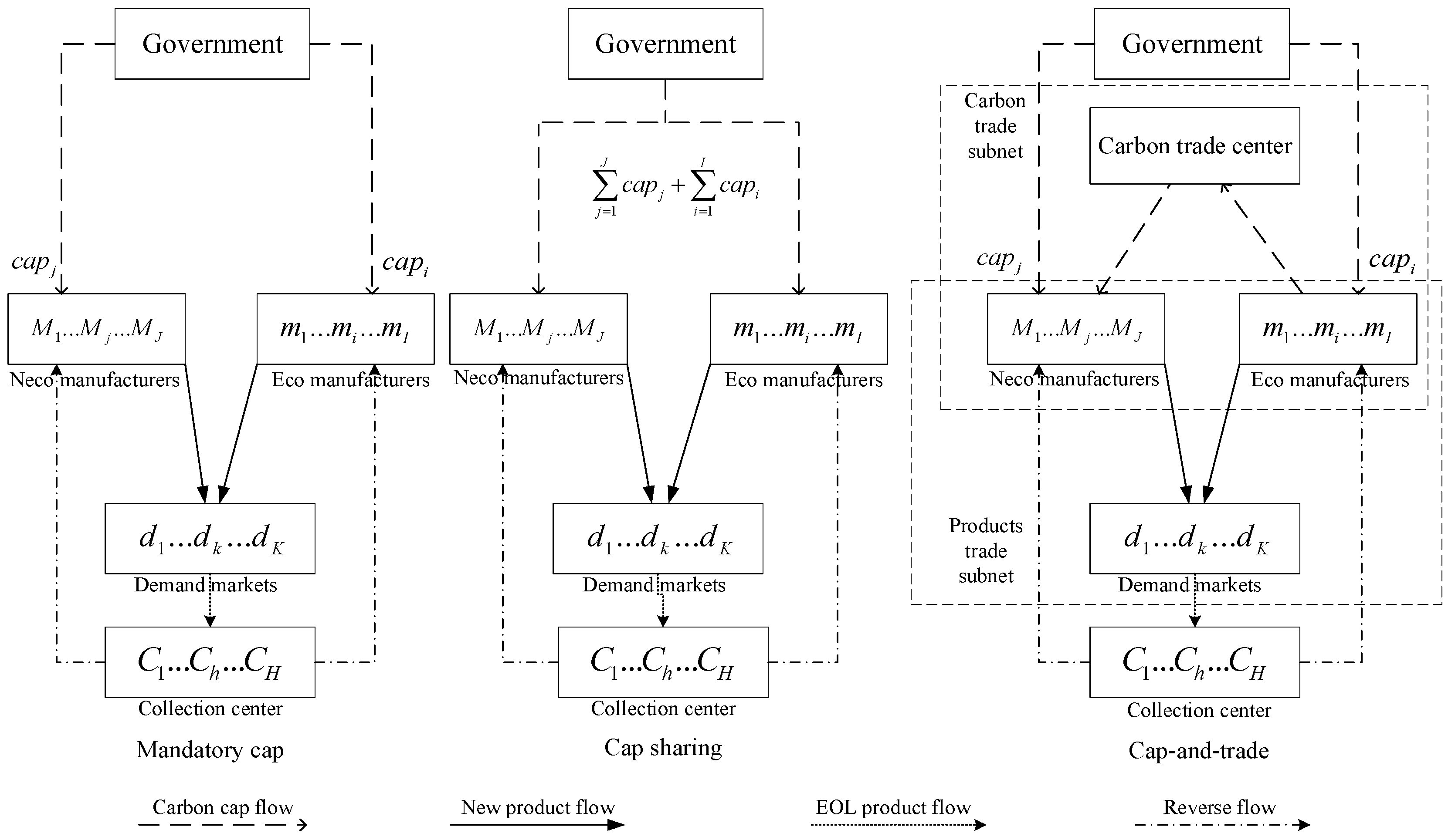
We first propose the carbon trade subnet and the product transaction subnet in the SCN and introduce the carbon trade center as a place for carbon trading.

(3)

By comparing three carbon reduction regulations, we illustrate the different laws of decision and profits and emission control and identify best practices for enterprises under different regulations.

We organized the remaining parts as follows. We provide a comparative discussion of the previous research highly related to our research in Section 2. Section 3 provides the notations and assumptions to accurately describe the decision models. In Section 4, the variational inequality models and the algorithm used to solve the models are described. Section 5 analyzes the results of numerical experiments to obtain the enlightenment of the management. Finally, we present the conclusions and suggestions in Section 6. The qualitative properties of the corresponding variational inequality models are presented in the Appendix C.

2. Literature Review

This paper focuses on sustainable supply chains, cap-and-trade regulations, non-cooperative equilibrium, and consumers’ environmental awareness. To better highlight our research issue, we briefly reviewed some relevant studies on these subjects. We will also point out the difference between our study and previous ones.

2.1. Sustainable Supply Chain

Pressure from stakeholders for sustainable development is forcing top management to reconsider its supply chain management, and the pursuit of sustainability has evolved as a popular trend in supply chain management [10,19]. Motivated by international retailers (e.g., Walmart and H&M) cooperating with their suppliers to reduce carbon emissions across supply chains, [10] investigated information sharing and studied its effect on carbon emission reduction. Considering a supply chain consisting of two competing manufacturers and a retailer, [20] studied the optimal green technology investment strategy problem of upstream manufacturers. Guo et al. [21] established a fashion supply chain consisting of one manufacturer and two competing retailers and discussed how retailer competition and consumer returns affect the development of green products in the fashion industry.

Recently, remanufacturing has come into focus as an area of economic and environmental insight [22,23,24,25]. Savaskan et al. [22] were among the first to divide the CLSC recycling model into the manufacturer recycling model, vendor recycling model, and third-party recycling model. The results of their work illustrated that the vendor recycling model is the most effective approach. Taleizadeh et al. [26] analyzed the effects of the third-party recycler in a CLSC under deterministic demand. Zerang et al. [27] established a three-echelon closed-loop supply chain model, and the results showed that the manufacturer-Stackelberg case is often the most effective scenario in CLSC.

Although the above-mentioned papers investigate the closed-loop supply chain in depth, the cap-and-trade regulation has been neglected as an effective approach to reducing carbon emissions, and thus needs further discussion.

2.2. Cap-and-Trade Regulations

To stimulate enterprises to actively reduce their carbon emissions through economic incentives, the government launched carbon trading, which can also be called cap-and-trade regulations. The European Union Emissions Trading Scheme (EU-ETS) is a successful form of cap-and-trade regulations. China launched its first carbon trading pilot in 2013, which entered into force in 2019. Therefore, it is important to explore the impacts of cap-and-trade regulations on enterprises, and conducting a simulation study on global carbon emission rights trading can provide practical outcomes [28,29,30,31,32,33,34,35]. Zhang and Xu [36] provided a basis for decision making on the reasonable use or sale of carbon emission rights by manufacturers and made a comparative analysis of the effectiveness of carbon trading and carbon tax. Du et al. [37] analyzed the game between decision-makers on product pricing and output considering cap-and-trade regulations and obtained a unique Nash equilibrium based on the basic Newsboy model. Yang et al. [38] and Yang et al. [39] both explored the channel selection problems under cap-and-trade regulations. The former asserts that products’ properties and consumers’ channel preferences are key factors affecting manufacturers’ channel selection. The latter highlights that both the level of carbon emissions reduction and the profits of manufacturers increase with the manufacturer’s product promotion.

Unlike our research, the above studies do not combine cap-and-trade regulations with reverse logistics. Moreover, they ignore the fact that carbon trade volume should be a decision variable in decision making.

2.3. Supply Chain Network Based on Non-Cooperative Equilibrium

The business crosses and fierce competition among supply chain members present the supply chain as a hierarchical network structure, including various enterprises and demand markets. With the coexistence of a competition and cooperation relationship, according to the rational person assumption, the corporate goal is to maximize its profits. Non-cooperative competition among the same types of members in the network forms a Nash equilibrium. Our study is also related to the literature rooted in supply chain network equilibrium under different environmental policies. In this field, scholars have carried out several studies on decision-making problems with different network structures [5,38,39]. Nagurney et al. [40] first established the SCN equilibrium model, making a great contribution to the promotion and application of supply chain network theory, and applied it to diverse fields [41,42]. With the implementation of environmental protection policies, He et al. [43] studied the joint effect of the mandatory cap policy and operational decision mode on profitability and emissions. The results illustrate that the cap-sharing scheme can achieve Pareto improvement for chain players’ profit and obtain a win-win situation for system profit and GHG emission reduction. Tao et al. [44] studied two types of mandatory cap policies under a multi-period scenario supply chain network and found that decision-makers can adjust their strategies under global carbon emissions constraints in most cases. He et al. [45] considered a supply chain super network constrained by a mandatory cap policy and examined the joint effect of stringent carbon regulations and operational decision modes on system performance.

2.4. Consumers’ Environmental Awareness

Currently, consumers are increasingly concerned about the energy crisis and global warming and are focused on environmentally friendly and green products [34,46]. In 2014, the Eurobarometer Commission survey stated that 75% of Europeans tended to buy green products at a higher price [47,48], which promotes the development of eco-friendly products. In China, a report by the AliResearch Institute found that the total number of consumers who have environmental awareness increased by 14% during 2011~2015, and reached 65 million in 2015 [49]. Consumers’ green preferences change their purchase behavior and promote low-carbon development [48]. Therefore, in this paper, the consumers’ environmental awareness level is introduced to depict the social environment more realistically.

2.5. Research Gap

We highlight the contribution of the aforementioned studies in

Table 1. Comparison of related research papers in low-carbon regulations.

Literature	Consumer’s Green Awareness	Low-Carbon Policy		Supply Chain Structure		Research Method
		Carbon Tax	Cap-and-Trade	SC	Network	Empirical Analysis	Modeling Analysis
1. [1]							√
2. [2]	√		√	√			√
3. [3]	√	√	√		√		√
4. [4]	√	√			√		√
5. [5]	√	√			√		√
6. [7]		√		√			√
7. [17]	√		√	√			√
8. [20]	√			√			√
9. [21]	√			√			√
10. [28]			√	√			√
11. [31]						√
12. [32]						√
13. [35]	√		√	√			√
14. [39]					√		√
15. [48]	√			√			√
16. [49]	√		√	√			√
This paper	√	Cap-and-trade, mandatory cap, cap sharing			√		√

. The literature review has shown that most previous studies examine the optimization of the supply chain under the given emission regulations. When a carbon cap exists, most studies consider it as a given constant that constrains manufacturers’ decision making. Most previous research related to carbon-constrained operations optimization only considers one or two kinds of carbon reduction policies. There is a lack of literature comparatively analyzing the impact of cap-and-trade regulations, mandatory cap policy, and cap-sharing schemes on multiple decision-makers under CLSCN.

To fill this gap, our study focuses on how different regulations influence members’ profits and carbon emissions in a CLSCN and investigate the remanufacturing’s impact on members’ equilibrium decisions. The results present meaningful information for the government to enact better carbon regulations and enterprises to adopt better operational policies.

3. Notations and Assumptions

3.1. Notations

The following parameters, decision variables, endogenous variables, and functions shown in

Table 2. Parameters of the model.

Parameters	Definition
$i$	$\mathrm{A} \mathrm{typical} \mathrm{ecological} \mathrm{manufacturer}, i=1,2,\cdot \cdot \cdot ,I$.
$j$	$\mathrm{A} \mathrm{typical} \mathrm{non}-\mathrm{ecological} \mathrm{manufacturer}, j=1,2,\cdot \cdot \cdot ,J$.
$k$	$\mathrm{A} \mathrm{typical} \mathrm{demand} \mathrm{market}, k=1,2,\cdot \cdot \cdot ,K$.
$h$	$\mathrm{A} \mathrm{typical} \mathrm{collection} \mathrm{center}, h=1,2,\cdot \cdot \cdot ,H$.
$\epsilon$	Unit carbon trading commission charged by carbon trading center.
$\omega$	Unit carbon trading price between non-eco manufacturers and eco manufacturers.
${\epsilon }_x$	$\mathrm{The} \mathrm{recycling} \mathrm{ratio} \mathrm{of} \mathrm{EOL} \mathrm{products} \mathrm{of} \mathrm{manufacturers} \mathrm{in} \mathrm{demand} \mathrm{markets},x=i,j$.
$\delta$	The proportion of reusable materials extracted from recycled products when collection centers dispose EOL products from demand markets.
${\beta }^x$	$x=r$$\mathrm{denotes} \mathrm{the} \mathrm{raw} \mathrm{material} \mathrm{conversion} \mathrm{ratio}, x=u$ denotes the reusable material conversion ratio.
$\sigma$	Consumer environmental awareness level.
$ca{p}_x$	$\mathrm{The} \mathrm{carbon} \mathrm{cap} \mathrm{of} \mathrm{manufacturers} \mathrm{allocated} \mathrm{by} \mathrm{the} \mathrm{government}, x=i,j$.
${\alpha }_x^y$	$\mathrm{The} \mathrm{carbon} \mathrm{emission} \mathrm{of} \mathrm{unit} \mathrm{product}. x=1$$\mathrm{denotes} \mathrm{non}-\mathrm{eco} \mathrm{product}, x=2$$\mathrm{denotes} \mathrm{eco} \mathrm{product}, y=i,j$.
${\tau }_t$	Carbon emission factor of a truck.
$x_s$	$\mathrm{The} \mathrm{distance} (\mathrm{in} \mathrm{km}) \mathrm{between} \mathrm{two} \mathrm{supply} \mathrm{chain} \mathrm{members}. s=jk,ik,hj,hi$.
$t_x$	$\mathrm{The} \mathrm{number} \mathrm{of} \mathrm{trucks} \mathrm{serving} \mathrm{different} \mathrm{transactions} \mathrm{in} \mathrm{the} \mathrm{CLSC} \mathrm{network}. x=1$$\mathrm{denotes} \mathrm{the} \mathrm{number} \mathrm{of} \mathrm{trucks} \mathrm{between} \mathrm{non}-\mathrm{ecological} \mathrm{manufacturers} \mathrm{and} \mathrm{demand} \mathrm{markets}; x=2$$\mathrm{denotes} \mathrm{the} \mathrm{number} \mathrm{of} \mathrm{trucks} \mathrm{between} \mathrm{non}-\mathrm{ecological} \mathrm{manufacturers} \mathrm{and} \mathrm{collection} \mathrm{centers}; x=3$$\mathrm{denotes} \mathrm{the} \mathrm{number} \mathrm{of} \mathrm{trucks} \mathrm{between} \mathrm{eco} \mathrm{manufacturers} \mathrm{and} \mathrm{demand} \mathrm{markets}; x=4$ denotes the number of trucks between eco manufacturers and collection centers.
$\rho$	The total transport costs of unit product.

,

Table 3. Decision variables of the model.

Decision Variables	Notations
$q_x^v$	$\mathrm{The} \mathrm{amount} \mathrm{of} \mathrm{raw} \mathrm{material} \mathrm{used} \mathrm{by} \mathrm{manufacturers} \mathrm{to} \mathrm{produce} \mathrm{new} \mathrm{products}, x=i,j,$${\mathit{q}}_j^v={\left(q_j^v\right)}_{J\times 1}\in R_{+}^J,$${\mathit{q}}_i^v={\left(q_i^v\right)}_{I\times 1}\in R_{+}^I$.
$q_x^u$	$\mathrm{The} \mathrm{amount} \mathrm{of} \mathrm{reusable} \mathrm{material} \mathrm{used} \mathrm{by} \mathrm{manufacturers} \mathrm{to} \mathrm{remanufacture} \mathrm{products}, x=i,j,$${\mathit{q}}_j^u={\left(q_j^u\right)}_{J\times 1}\in R_{+}^J,$${\mathit{q}}_i^u={\left(q_i^u\right)}_{I\times 1}\in R_{+}^I$.
$q_{jk}$	The amount of products that a non-ecological manufacturer j sells and transfers to demand market k, ${\mathit{Q}}_1={\left(q_{jk}\right)}_{JK\times 1}\in R_{+}^{JK}$.
$q_{hj}^u$	The amount of reusable material from collection center h to non-ecological manufacturer j, ${\mathit{Q}}_2={\left(q_{hj}^u\right)}_{HJ\times 1}\in R_{+}^{HJ}$.
$q_{ik}$	The amount of product that ecological manufacturer i sells and transfers to demand market k, ${\mathit{Q}}_3={\left(q_{ik}\right)}_{IK\times 1}\in R_{+}^{IK}$.
$q_{hi}^u$	The amount of reusable material from collection center h to ecological manufacturer i, ${\mathit{Q}}_4={\left(q_{hi}^u\right)}_{HI\times 1}\in R_{+}^{HI}$.
$q_{kh}^u$	The amount of recycling EOL (end of life) product from demand market k to collection center h, ${\mathit{Q}}_5={\left(q_{kh}^u\right)}_{KH\times 1}\in R_{+}^{KH}$.
$t_j$	The carbon cap amount of non-ecological manufacturer j buying from carbon trade center, ${\mathit{T}}_1={(t_j)}_{J\times 1}\in R_{+}^J$.
$t_i$	The carbon cap amount of ecological manufacturer i selling to carbon trade center, ${\mathit{T}}_2={(t_i)}_{I\times 1}\in R_{+}^I$.
${\rho }_k^j$	The price consumers paid for non-ecological products in demand market k, and ${\mathit{\rho }}^J={\left({\rho }_k^j\right)}_{K\times 1}\in R_{+}^K$.
${\rho }_k^i$	The price consumers paid for ecological products in demand market k, and ${\mathit{\rho }}^I={\left({\rho }_k^i\right)}_{K\times 1}\in R_{+}^K$.

,

Table 4. Endogenous variables of the model.

Endogenous Variables	Notations
${\rho }_{xk}$	The product price between manufacturers and demand market k, $x=i,j$.
${\rho }_{hk}$	The EOL product recycling price paid by collection center h to consumers in demand market k.
${\rho }_{hj}$	The reusable material price paid by non-ecological manufacturer j to collection center h.
${\rho }_{hi}$	The reusable material price paid by ecological manufacturer i to collection center h.

and

Table 5. Functions of the model.

Functions	Notations
$f_x=f_x({\beta }^r,{\mathit{q}}_x^v)$	$\mathrm{The} \mathrm{production} \cos \mathrm{t} \mathrm{function} \mathrm{of} \mathrm{manufacturers} \mathrm{x}, x=i,j$.
$f_x^u=f_x^u({\beta }^u,{\mathit{q}}_x^u)$	$\mathrm{The} \mathrm{remanufacturing} \cos \mathrm{t} \mathrm{function} \mathrm{of} \mathrm{manufacturers} \mathrm{x}, x=i,j$.
$c_{xk}=c_{xk}(q_{xk})$	$\mathrm{The} \mathrm{transaction} \cos \mathrm{t} \mathrm{function} \mathrm{from} \mathrm{manufacturers} \mathrm{x} \mathrm{to} \mathrm{demand} \mathrm{market} \mathrm{k}, x=i,j$.
$c_{xk}^K=c_{xk}^K(q_{xk})$	The transportation cost burden assumed by consumers to obtain the product.
$c_x^t=c_x^t(t_x)$	$\mathrm{The} \mathrm{carbon} \mathrm{transaction} \cos \mathrm{t} \mathrm{undertaken} \mathrm{by} \mathrm{carbon} \mathrm{trade} \mathrm{center}, x=i,j$.
$c_{hx}^u=c_{hx}^u(q_{hx}^u)$	$\mathrm{The} \mathrm{transaction} \cos \mathrm{t} \mathrm{from} \mathrm{collection} \mathrm{center} \mathrm{to} \mathrm{manufacturers}, x=i,j$.
$c_h=c_h(q_{kh}^u)$	The disposal cost function of collection center h.
$c_{kh}=c_{kh}(q_{kh}^u)$	The transaction cost from demand market k to collection center h.
${\alpha }_k^u({\mathit{Q}}_5)$	Disutility to consumers due to collection of EOL product.
$d_k^l=d_k^l({\rho }^I,{\rho }^J,\sigma )$	The demand function of ecological product.
$d_k^h=d_k^h({\rho }^J,{\rho }^I)$	The demand function of non-ecological product.

are used throughout the remainder of this paper.

3.2. Assumptions

To highlight the research question of the models developed later in Section 4, some assumptions need to be presented as follows.

Assumption 1.

The manufacturers are divided into two types called “non-eco manufacturer” and “eco manufacturer” according to whether they adopt green production technology. Eco manufacturers undertake higher production costs than non-eco manufacturers due to their possession of better production technology to decrease carbon emissions, and two products have a certain substitution relationship [50]. This assumption comes from reality (e.g., Huawei mobiles phones and Apple mobile phones). As it can be seen in the demand function:

$$d_k^l=250-2{\rho }_k^l-1.5{\rho }_{3-k}^l+0.5({\rho }_k^h+{\rho }_{3-k}^h)+\sigma \psi {\displaystyle \sum _{x=1}^2(1-{\alpha }_x^I)};d_k^h=230-2{\rho }_k^h-1.5{\rho }_{3-k}^h+0.5({\rho }_k^l+{\rho }_{3-k}^l)+\sigma \psi {\displaystyle \sum _{x=1}^2(1-{\alpha }_x^J)}$$

the quantity of each kind of product is affected by both its own and another product’s selling price, which represents the substitution relationship between them.

Assumption 2.

The new product and remanufactured product are homogeneous [51,52]. However, re-manufactured products have lower production costs and unit carbon emissions than the new ones. This assumption refers to the literature [22,53,54]. Savaskan et al. used the Eastman Kodak Company example to illustrate this relationship. Used cameras are typically upgraded to the quality of new ones, and both products can perfectly substitute each other. In this paper, we address the carbon emissions in the production process; thus, different types of products emit the same carbon dioxide when used.

Assumption 3.

Carbon emissions are generated during both the production and transportation processes [50]. To avoid trivial cases and to focus on the goals of this research, we only consider the total carbon emissions of each truck and do not carry out further analyses on the distance covered by vehicles.

Assumption 4.

The carbon quota allocation mechanism is based on “Benchmarking,” which can be more effective in pushing facilities to reduce carbon emissions [2,55]. Under cap-and-trade regulations, caps can be sold or bought to satisfy the target production [2].

Assumption 5.

The consumers’ environmental awareness level is reflected in the demand function [56,57].

Assumption 6.

The cost functions in this paper are all continuous differentiable convex functions [40,58].

4. Model

In this paper, we consider three scenarios of carbon reduction regulations. The mandatory cap policy requires manufacturers not to emit more than a specific quota. Otherwise, the firm will face heavy penalties that force it to comply with the policy. As for the cap sharing policy, the total carbon emissions of different firms cannot exceed the aggregate quota of these firms; the carbon quotas can be transferred freely between two types of manufacturers. The cap-and-trade policy requires a carbon trade market that charges a certain commission from the enterprises participating in the carbon transaction and seeks maximum profit.

In addition, the European Commission is willing to regulate heavy-duty vehicles’ carbon emissions; this willingness is modeled in this paper. Trucks are only supposed to be used in the main logistics phases: (1) forward logistics: transferring products from manufacturers to customers; (2) reverse logistics: transferring reusable raw materials from collection centers to manufacturers. As assumed in [59], transferring EOL products from demand markets to collection centers is undertaken by smaller dimension vans that are not regulated strictly.

In the following, we construct three equilibrium models according to different policies, and the different closed-loop supply chain network structures are shown in Figure 1.

4.1. Demand Market Decisions

Demand markets are the final demand points of product transaction in forward flow and are also the source of EOL products in reverse flow. In a forward transaction, consumers of each demand market decide the quantity of non-eco products and eco products that they want to buy according to the prices charged by manufacturers and transaction costs. In a reverse transaction, consumers sell the EOL products to collection centers when the recycling prices are reasonable and can compensate for the loss of consumers caused by recycling.

According to the previous functions and notations definition, for the non-eco products in demand market $k$, we have the following complementary relationships:

$${\rho }_{jk}^{*}+c_{jk}^{K*}\{\begin{array}{c}={\rho }_k^{h*}, \mathrm{if} q_{jk}^{*}>0\\ \ge {\rho }_k^{h*}, \mathrm{if} q_{jk}^{*}=0\end{array}$$

(1)

$$d_k^h\{\begin{array}{c}={\displaystyle \sum _{j=1}^J{q}_{jk}^{*}}, \mathrm{if} {\rho }_k^{h*}>0\\ \le {\displaystyle \sum _{j=1}^J{q}_{jk}^{*}}, \mathrm{if} {\rho }_k^{h*}=0\end{array}$$

(2)

When the transactions between non-eco manufacturers and demand markets occur, $q_{jk}^{*}>0$ and ${\rho }_k^{h*}>0$ hold simultaneously, and the demand and supply are equal. Otherwise, the transactions cannot occur.

Similarly, for the eco products, we have:

$${\rho }_{ik}^{*}+c_{ik}^{K*}\{\begin{array}{c}={\rho }_k^{l*}, \mathrm{if} q_{ik}^{*}>0\\ \ge {\rho }_k^{l*}, \mathrm{if} q_{ik}^{*}=0\end{array}$$

(3)

$$d_k^l\{\begin{array}{c}={\displaystyle \sum _{i=1}^I{q}_{ik}^{*}}, \mathrm{if} {\rho }_k^{l*}>0\\ \le {\displaystyle \sum _{i=1}^I{q}_{ik}^{*}}, \mathrm{if} {\rho }_k^{l*}=0\end{array}$$

(4)

In the reverse logistics, after the consumption process, part of the products become EOL products that have no use value and can be recycled. When these EOL products are sent to collection centers, it will bring disutility to consumers. We assume ${\alpha }_k^u({\mathit{Q}}_5)$ is a monotonically increasing function that depends on the collected volume vector ${\mathit{Q}}_5$, which means more EOL products collection brings higher consumers’ disutility. Further, the more recycling products are recycled by collection centers, the higher the buy-back prices are. If the buy-back price ${\rho }_{kh}^{u*}$ can compensate the disutility of consumers, that is, ${\rho }_{kh}^{u*}={\alpha }_k^u({\mathit{Q}}_5^{*})$, then recycling transactions will occur; otherwise, recycling transactions will not occur. This relationship can be described as the following complementary form:

$${\alpha }_k^u({\mathit{Q}}_5^{*})\{\begin{array}{c}={\rho }_{kh}^{u*}, \mathrm{if} q_{kh}^{u*}>0\\ \ge {\rho }_{kh}^{u*}, \mathrm{if} q_{kh}^{u*}=0\end{array}$$

(5)

$$s.t.{\displaystyle \sum _{h=1}^H{q}_{kh}^u}\le {\epsilon }_j{\displaystyle \sum _{j=1}^J{q}_{jk}}+{\epsilon }_i{\displaystyle \sum _{i=1}^I{q}_{ik}}$$

(6)

Constraint (6) indicates that the products in reverse logistics are always less than those in forward logistics.

Integrating the forward and reverse behavior of consumers, the optimality conditions of demand markets can be defined as follows: determine the optimal solution $({\mathit{Q}}_1^{*},{\mathit{Q}}_3^{*},{\mathit{\rho }}^{J*},{\mathit{\rho }}^{I*},{\mathit{Q}}_5^{*},{\mathit{\gamma }}^{*})\in {\mathsf{\Omega }}_k$, satisfying:

$$\begin{array}{l}{\displaystyle \sum _{j=1}^J{\displaystyle \sum _{k=1}^K\left[{\rho }_{jk}^{*}+c_{jk}^{K*}-{\rho }_k^{h*}-{\epsilon }_j{\gamma }_k^{*}\right]}\times \left[q_{jk}-q_{jk}^{*}\right]}+{\displaystyle \sum _{i=1}^I{\displaystyle \sum _{k=1}^K\left[{\rho }_{ik}^{*}+c_{ik}^{K*}-{\rho }_k^{l*}-{\epsilon }_i{\gamma }_k^{*}\right]}}\times \left[q_{ik}-q_{ik}^{*}\right]+\\ {\displaystyle \sum _{k=1}^K\left[{\displaystyle \sum _{j=1}^J{q}_{jk}^{*}}-d_k^{h*}\right]}\times \left[{\rho }_k^h-{\rho }_k^{h*}\right]+{\displaystyle \sum _{k=1}^K\left[{\displaystyle \sum _{i=1}^I{q}_{ik}^{*}}-d_k^{l*}\right]}\times \left[{\rho }_k^l-{\rho }_k^{l*}\right]+\\ {\displaystyle \sum _{h=1}^H{\displaystyle \sum _{k=1}^K\left[{\alpha }_k^u({\mathit{Q}}_5^{*})-{\rho }_{kh}^{u*}+{\gamma }_k^{*}\right]}\times \left[q_{kh}^u-q_{kh}^{u*}\right]}+{\displaystyle \sum _{k=1}^K\left[{\epsilon }_j{\displaystyle \sum _{j=1}^J{q}_{jk}^{*}}+{\epsilon }_i{\displaystyle \sum _{i=1}^I{q}_{ik}^{*}}-{\displaystyle \sum _{k=1}^K{q}_{kh}^{u*}}\right]}\times \left[{\gamma }_k-{\gamma }_k^{*}\right]\ge 0.\\ \forall ({\mathit{Q}}_1,{\mathit{Q}}_3,{\mathit{\rho }}^J,{\mathit{\rho }}^I,{\mathit{Q}}_5,\mathit{\gamma })\in {\mathsf{\Omega }}_k\end{array}$$

(7)

where ${\mathsf{\Omega }}_k=R_{+}^{JK+IK+J+I+KH+K}$, ${\gamma }_k$ is the Lagrangian multiplier corresponding to Constraint (6), and $\mathit{\gamma }={\left({\gamma }_k\right)}_{K\times 1}\in R_{+}^K$.

4.2. Collection Centers’ Decisions

In the reverse logistics, the collection center $h$ recycles these EOL products by paying price ${\rho }_{kh}^u$ to consumers in demand markets. After separating, detecting, and other treatments, these EOL products are transformed to various reusable materials and then are sold to manufacturers at price ${\rho }_{hj}^u$ and ${\rho }_{hi}^u$, respectively. Therefore, the collection center $h$ needs to decide the recycling quantity of EOL products and the sold quantity of reusable materials. Collection center $h$ seeks to maximize its profit that can be described as:

$$max\left[{\displaystyle \sum _{j=1}^J{\rho }_{hj}^{u*}{q}_{hj}^u}+{\displaystyle \sum _{i=1}^I{\rho }_{hi}^{u*}{q}_{hi}^u}-{\displaystyle \sum _{k=1}^K\left({\rho }_{kh}^{u*}{q}_{kh}^u+c_{kh}\right)}-c_h\right]$$

(8)

$$s.t. {\displaystyle \sum _{j=1}^J{q}_{hj}^u}+{\displaystyle \sum _{i=1}^I{q}_{hi}^u}\le \delta {\displaystyle \sum _{k=1}^K{q}_{kh}^u}$$

(9)

The objective function is the difference of the revenues and costs. The revenues are ${\displaystyle \sum _{j=1}^J{\rho }_{hj}^{u*}{q}_{hj}^u}+{\displaystyle \sum _{i=1}^I{\rho }_{hi}^{u*}{q}_{hi}^u}$ resulting from selling reusable materials to non-eco manufacturers and eco manufacturers at prices ${\rho }_{hj}^{u*}$ and ${\rho }_{hi}^{u*}$, respectively. The costs include the buy-back price ${\displaystyle \sum _{k=1}^K{\rho }_{kh}^{u*}{q}_{kh}^u}$ paid for consumers in demand markets, the disposal cost $c_h$, and the transaction cost $c_{kh}$. Constraint (9) ensures the trade-off between manufacturing and re-manufacturing. Finally, all decision variables are non-negative.

All collection centers compete in a non-cooperative manner, and all functions related are assumed continuous and convex. The optimal conditions of all collection centers can be expressed as following variational inequality: determine the optimal solution $({\mathit{Q}}_2^{*},{\mathit{Q}}_4^{*},{\mathit{Q}}_5^{*},{\mathit{\lambda }}^{*})\in {\mathsf{\Omega }}_h$, satisfying:

$$\begin{array}{l}{\displaystyle \sum _{j=1}^J{\displaystyle \sum _{h=1}^H\left[{\lambda }_h^{*}-{\rho }_{hj}^{u*}\right]}}\times \left[q_{hj}^u-q_{hj}^{u*}\right]+{\displaystyle \sum _{i=1}^I{\displaystyle \sum _{h=1}^H\left[{\lambda }_h^{*}-{\rho }_{hi}^{u*}\right]}\times }\left[q_{hi}^u-q_{hi}^{u*}\right]+\\ {\displaystyle \sum _{h=1}^H{\displaystyle \sum _{k=1}^K\left[\frac{\partial c_{kh}^{*}}{\partial q_{kh}^u}+\frac{\partial c_h^{*}}{\partial q_{kh}^u}+{\rho }_{kh}^{u*}-\delta {\lambda }_h^{*}\right]}}\times \left[q_{kh}^u-q_{kh}^{u*}\right]+{\displaystyle \sum _{h=1}^H\left[\delta {\displaystyle \sum _{k=1}^K{q}_{kh}^{u*}}-{\displaystyle \sum _{j=1}^J{q}_{hj}^{u*}}-{\displaystyle \sum _{i=1}^I{q}_{hi}^{u*}}\right]}\times \left[{\lambda }_h-{\lambda }_h^{*}\right]\ge 0.\end{array}$$

(10)

$$\forall ({\mathit{Q}}_2,{\mathit{Q}}_4,{\mathit{Q}}_5,\lambda )\in {\mathsf{\Omega }}_h$$

where ${\mathsf{\Omega }}_h=R_{+}^{HJ+HI+KH+H}$, ${\lambda }_h$ is the Lagrangian multiplier corresponding to constraint (9), and $\mathit{\lambda }={\left({\lambda }_h\right)}_{H\times 1}\in R_{+}^H$.

4.3. The Supply Chain Network under Cap-and-Trade (CT) Policy

Under the cap-and-trade policy, we assume that the unit carbon quota price is exogenous and remains unchanged.

4.3.1. Non-Ecological Manufacturers’ Decisions

We first study non-eco manufacturers’ decisions. According to the previous Assumption 4, the non-eco manufacturer $j$ needs to buy the quota that can be expressed as $t_j={\alpha }_1^J{\beta }^r{q}_j^v+{\alpha }_2^J{\beta }^u{q}_j^u+t_1{\tau }_t{\displaystyle \sum _{k=1}^K{x}_{jk}{q}_{jk}}+t_2{\tau }_t{\displaystyle \sum _{h=1}^H{x}_{hj}{q}_{hj}^u}-ca{p}_j$, the corresponding payment is $\epsilon t_j+\omega t_j$. When manufacturer $j$ pursues the maximization of profit, the objective function can be represented as:

$$max\left[{\displaystyle \sum _{k=1}^K\left({\rho }_{jk}^{*}{q}_{jk}-c_{jk}\right)-{\displaystyle \sum _{h=1}^H\left({\rho }_{hj}^{u*}{q}_{hj}^u+c_{hj}\right)}-f_j-f_j^u-\rho \left(t_1{\displaystyle \sum _{k=1}^K{x}_{jk}{q}_{jk}}+t_2{\displaystyle \sum _{h=1}^H{x}_{hj}{q}_{hj}^u}\right)-\epsilon t_j-\omega t_j}\right]$$

(11)

$$s.t. q_j^u\le {\displaystyle \sum _{h=1}^H{q}_{hj}^u}$$

(12)

$${\displaystyle \sum _{k=1}^K{q}_{jk}\le {\beta }^r{q}_j^v+{\beta }^u{q}_j^u}$$

(13)

$${\alpha }_1^J{\beta }^r{q}_j^v+{\alpha }_2^J{\beta }^u{q}_j^u+t_1{\tau }_t{\displaystyle \sum _{k=1}^K{x}_{jk}{q}_{jk}}+t_2{\tau }_t{\displaystyle \sum _{h=1}^H{x}_{hj}{q}_{hj}^u}-ca{p}_j-t_j=0$$

(14)

Constraint (14) ensures that the manufacturer $j$’s total carbon emissions are equal to the sum of $ca{p}_j$ and $t_j$.

Based on the CT model, in this case, manufacturer $j$ needs to make an additional decision regarding the carbon transaction amount $t_j$. Hence, the optimum solution of the above objective function is characterized by the following variational inequality with $({\mathit{q}}_j^{v*},{\mathit{q}}_j^{u*},{\mathit{Q}}_1^{*},{\mathit{Q}}_2^{*},{\mathit{T}}_1^{*},{\mathit{\phi }}_1^{*},{\mathit{\phi }}_2^{*},{\mathit{\phi }}_3^{*})\in {\mathsf{\Omega }}_J^1$, such that:

$$\begin{array}{l}{\displaystyle \sum _{j=1}^J\left[\frac{\partial f_j^{*}}{\partial q_j^v}-{\beta }^r{\phi }_j^{2*}-{\alpha }_1^J{\beta }^r{\phi }_j^{3*}\right]\times \left[q_j^v-q_j^{v*}\right]}+\\ {\displaystyle \sum _{j=1}^J\left[\frac{\partial f_j^{u*}}{\partial q_j^u}+{\phi }_j^{1*}-{\beta }^u{\phi }_j^{2*}-{\alpha }_2^J{\beta }^u{\phi }_j^{3*}\right]}\times \left[q_j^u-q_j^{u*}\right]+\\ {\displaystyle \sum _{j=1}^J{\displaystyle \sum _{k=1}^K\left[\frac{\partial c_{jk}^{*}}{\partial q_{jk}}-{\rho }_{jk}^{*}+\rho t_1{x}_{jk}+{\phi }_j^{2*}-t_1{\tau }_t{x}_{jk}{\phi }_j^{3*}\right]\times \left[q_{jk}-q_{jk}^{*}\right]}}+\\ {\displaystyle \sum _{j=1}^J{\displaystyle \sum _{h=1}^H\left[\frac{\partial c_{hj}^{u*}}{\partial q_{hj}^u}+{\rho }_{hj}^{u*}+\rho t_2{x}_{hj}-{\phi }_j^{1*}-t_2{\tau }_t{x}_{hj}{\phi }_j^{3*}\right]}}\times \left[q_{hj}^u-q_{hj}^{u*}\right]+\\ {\displaystyle \sum _{j=1}^J\left[\epsilon +\omega +{\phi }_j^{3*}\right]}\times \left[t_j-t_j^{*}\right]+{\displaystyle \sum _{j=1}^J\left[{\displaystyle \sum _{h=1}^H{q}_{hj}^{u*}}-q_j^{u*}\right]}\times \left[{\phi }_j^1-{\phi }_j^{1*}\right]+\\ {\displaystyle \sum _{j=1}^J\left[{\beta }^r{q}_j^{v*}+{\beta }^u{q}_j^{u*}-{\displaystyle \sum _{k=1}^K{q}_{jk}^{*}}\right]}\times \left[{\phi }_j^2-{\phi }_j^{2*}\right]+\\ {\displaystyle \sum _{j=1}^J\left[{\alpha }_1^J{\beta }^r{q}_j^{v*}+{\alpha }_2^J{\beta }^u{q}_j^{u*}+t_1{\tau }_t{\displaystyle \sum _{k=1}^K{x}_{jk}{q}_{jk}^{*}}+t_2{\tau }_t{\displaystyle \sum _{h=1}^H{x}_{hj}{q}_{hj}^{u*}}-ca{p}_j-t_j^{*}\right]}\times \left[{\phi }_j^3-{\phi }_j^{3*}\right]\ge 0.\end{array}$$

(15)

$$\forall ({\mathit{q}}_j^v,{\mathit{q}}_j^u,{\mathit{Q}}_1,{\mathit{Q}}_2,{\mathit{T}}_1,{\mathit{\phi }}_1,{\mathit{\phi }}_2,{\mathit{\phi }}_3)\in {\mathsf{\Omega }}_J^1$$

where ${\mathsf{\Omega }}_J^1=R_{+}^{2J+JK+HJ+3J}\times R^J$. Note that ${\phi }_j^1$, ${\phi }_j^2$, and ${\phi }_j^3$ are the Lagrangian multiplier associated with Constraint (12), Constraint (13), and Constraint (14), respectively, while ${\mathit{\phi }}_1={\left({\phi }_j^1\right)}_{J\times 1}\in R_{+}^J$, ${\mathit{\phi }}_2={\left({\phi }_j^2\right)}_{J\times 1}\in R_{+}^J$, ${\mathit{\phi }}_3={\left({\phi }_j^3\right)}_{J\times 1}\in R^J$.

To explore the significance of management, we give some explanations for VI (15). From the 3rd term of VI (15), we have ${\rho }_{jk}^{*}=\frac{\partial c_{jk}^{*}}{\partial q_{jk}}+\rho t_1{x}_{jk}+{\phi }_j^{2*}-t_1{\tau }_t{x}_{jk}{\phi }_j^{3*}$ when $q_{jk}^{*}>0$; in other words, the transaction price between non-ecological manufacturer $j$ and demand market $k$ comprises a marginal transaction cost, unit truck transportation cost, and related carbon emission factor. From the 1st term of VI (15), we have ${\phi }_j^{2*}=\frac{1}{{\beta }^r}\left(\frac{\partial f_j^{*}}{\partial q_j^v}-{\alpha }_1^J{\beta }^r{\phi }_j^{3*}\right)$ when $q_j^{v*}>0$, and are mainly marginal production costs. Therefore, the previous stage cost transmits to the next stage by the transaction price.

A point that is necessary to show is that the corresponding Lagrangian multipliers of Constraint (14) may be negative because Constraint (14) is an equation. In addition, $t_j^{*}$ is affected by the sum of $\epsilon$ and $\omega$.

4.3.2. Ecological Manufacturers’ Decisions

Similarly, the surplus carbon quotas of the eco manufacturer can be expressed as $t_i=ca{p}_i-{\alpha }_1^I{\beta }^r{q}_i^v-{\alpha }_2^I{\beta }^u{q}_i^u-t_3{\tau }_t{\displaystyle \sum _{k=1}^K{x}_{ik}{q}_{ik}}-t_4{\tau }_t{\displaystyle \sum _{h=1}^H{x}_{hi}{q}_{hi}^u}$. We, therefore, obtain the manufacturer $i$’s objective below to maximize its profit through aggregate revenue minus costs:

$$max\left[{\displaystyle \sum _{k=1}^K\left({\rho }_{ik}^{*}{q}_{ik}-c_{ik}\right)-{\displaystyle \sum _{h=1}^H\left({\rho }_{hi}^{*}{q}_{hi}^u+c_{hi}\right)}-f_i-f_i^u-\rho \left(t_3{\displaystyle \sum _{k=1}^K{x}_{ik}{q}_{ik}}+t_4{\displaystyle \sum _{h=1}^H{x}_{hi}{q}_{hi}^u}\right)-\epsilon t_i+\omega t_i}\right]$$

(16)

$$s.t. q_i^u\le {\displaystyle \sum _{h=1}^H{q}_{hi}^u}$$

(17)

$${\displaystyle \sum _{k=1}^K{q}_{ik}\le {\beta }^r{q}_i^v+{\beta }^u{q}_i^u}$$

(18)

$$ca{p}_i-{\alpha }_1^I{\beta }^r{q}_i^v-{\alpha }_2^I{\beta }^u{q}_i^u-t_3{\tau }_t{\displaystyle \sum _{k=1}^K{x}_{ik}{q}_{ik}}-t_4{\tau }_t{\displaystyle \sum _{h=1}^H{x}_{hi}{q}_{hi}^u}=t_i$$

(19)

The last item of objective function $\omega t_i$ denotes the manufacturer $i$’s extra revenue. Constraint (19) ensures that the total carbon emissions of manufacturer $i$ plus $t_i$ equals $ca{p}_i$. In this case, manufacturer $i$ needs to make an additional decision on the carbon transaction amount $t_i$. Therefore, the optimum solution of the above objective function can be characterized by the following variational inequality with $({\mathit{q}}_i^{v*},{\mathit{q}}_i^{u*},{\mathit{Q}}_3^{*},{\mathit{Q}}_4^{*},{\mathit{T}}_2^{*},{\mathit{\varphi }}_1^{*},{\mathit{\varphi }}_2^{*},{\mathit{\varphi }}_3^{*})\in {\mathsf{\Omega }}_I^1$:

$$\begin{array}{l}{\displaystyle \sum _{i=1}^I{\displaystyle \sum _{k=1}^K\left[\frac{\partial c_{ik}^{*}}{\partial q_{ik}}-{\rho }_{ik}^{*}+\rho t_3{x}_{ik}+{\varphi }_i^{2*}+t_3{\tau }_t{x}_{ik}{\varphi }_i^{3*}\right]}}\times \left[q_{ik}-q_{ik}^{*}\right]+\\ {\displaystyle \sum _{i=1}^I{\displaystyle \sum _{h=1}^H\left[\frac{\partial c_{hi}^{u*}}{\partial q_{hi}^u}+{\rho }_{hi}^{u*}+\rho t_4{x}_{hi}-{\varphi }_i^{1*}+t_4{\tau }_t{x}_{hi}{\varphi }_i^{3*}\right]}}\times \left[q_{hi}^u-q_{hi}^{u*}\right]+\\ {\displaystyle \sum _{i=1}^I\left[\epsilon -\omega +{\varphi }_i^{3*}\right]}\times \left[t_i-t_i^{*}\right]+{\displaystyle \sum _{i=1}^I\left[{\displaystyle \sum _{h=1}^H{q}_{hi}^{u*}}-q_i^{u*}\right]}\times \left[{\varphi }_i^1-{\varphi }_i^{1*}\right]+\\ {\displaystyle \sum _{i=1}^I\left[{\beta }^r{q}_i^{v*}+{\beta }^u{q}_i^{u*}-{\displaystyle \sum _{k=1}^K{q}_{ik}^{*}}\right]}\times \left[{\varphi }_i^2-{\varphi }_i^{2*}\right]+\\ {\displaystyle \sum _{i=1}^I\left[ca{p}_i-{\alpha }_1^I{\beta }^r{q}_i^v-{\alpha }_2^I{\beta }^u{q}_i^u-t_3{\tau }_t{\displaystyle \sum _{k=1}^K{x}_{ik}{q}_{ik}}-t_4{\tau }_t{\displaystyle \sum _{h=1}^H{x}_{hi}{q}_{hi}^u}-t_i\right]}\times \left[{\varphi }_i^3-{\varphi }_i^{3*}\right]\ge 0.\end{array}$$

(20)

$$\forall ({\mathit{q}}_i^v,{\mathit{q}}_i^u,{\mathit{Q}}_3,{\mathit{Q}}_4,{\mathit{T}}_2,{\mathit{\varphi }}_1,{\mathit{\varphi }}_2,{\mathit{\varphi }}_3)\in {\mathsf{\Omega }}_I^1$$

where ${\mathsf{\Omega }}_I^1=R_{+}^{2I+IK+HI+2I}\times R^I$. Note that ${\varphi }_i^1$, ${\varphi }_i^2$ and ${\varphi }_i^3$ are the Lagrangian multipliers associated with Constraint (17), Constraint (18), and Constraint (19), respectively, while ${\mathit{\varphi }}_1={\left({\varphi }_i^1\right)}_{I\times 1}\in R_{+}^I$, ${\mathit{\varphi }}_2={\left({\varphi }_i^2\right)}_{I\times 1}\in R_{+}^I$, ${\mathit{\varphi }}_3={\left({\varphi }_i^3\right)}_{I\times 1}\in R^I$.

4.3.3. Carbon Trade Center’s Decisions

Carbon trade centers charge a certain fee $\epsilon$ for unit carbon trade volume. Simultaneously, carbon trade centers should undertake associated cost ${\displaystyle {\sum }_{j=1}^J{c}_j^t}+{\displaystyle {\sum }_{i=1}^I{c}_i^t}$. The carbon trade center also pursues profit maximization, which can be described as:

$$max\left[{\displaystyle \sum _{j=1}^J(\epsilon t_j^{*}-c_j^t(t_j^{*}))+{\displaystyle \sum _{i=1}^I(\epsilon t_i^{*}-c^t{}_i(t_i^{*}))}}\right]$$

(21)

$$s.t. {\displaystyle \sum _{j=1}^J{t}_j}\le {\displaystyle \sum _{i=1}^I{t}_i}$$

(22)

Constraint (22) shows the balance between the demand supply of the carbon quota. The profit of the carbon trade center seeking to maximize can be transformed into the following variational inequality: determine the optimal solution $\forall ({\mathit{T}}_1^{*},{\mathit{T}}_2^{*},{\zeta }_c^{*})\in {\mathsf{\Omega }}_c$, satisfying:

$${\displaystyle \sum _{j=1}^J\left[\frac{\partial c_j^{t*}}{\partial t_j}+{\lambda }_c^{*}-\epsilon \right]}\times \left[t_j-t_j^{*}\right]+{\displaystyle \sum _{i=1}^I\left[\frac{\partial c_i^{t*}}{\partial t_i}-\epsilon -{\lambda }_c^{*}\right]}\times \left[t_i-t_i^{*}\right]+\left[{\displaystyle \sum _{i=1}^I{t}_i^{*}}-{\displaystyle \sum _{j=1}^J{t}_j^{*}}\right]\times \left[{\lambda }_c-{\lambda }_c^{*}\right]\ge 0.$$

(23)

$$\forall ({\mathit{T}}_1,{\mathit{T}}_2,{\zeta }_c)\in {\mathsf{\Omega }}_c$$

where ${\mathsf{\Omega }}_c=R_{+}^{J+I+1}$. Note that ${\zeta }_c$ is the Lagrangian multiplier associated with Constraint (22) and ${\zeta }_c\in R_{+}$.

4.3.4. The Equilibrium Conditions of Closed-Loop Supply Chain Network in the CT Model

Under the cap-and-trade regulations, for the closed-loop supply chain network, the Nash equilibrium (Nash 1950) conditions of VI (7), VI (10), VI (15), VI (20), and VI (23) must hold simultaneously, and no one gains more from altering the current strategies.

Definition 1.

The equilibrium of the CLSCN under cap-and-trade regulation occurs when the sum of the left-hand side (L.H.S.) of (7), L.H.S. of (10), L.H.S. of (15), L.H.S. of (20), and L.H.S. of (23) is non-negative.

Theorem 1.

The equilibrium conditions of the CLSCN under cap-and-trade regulations are equivalent to the solutions of VI as follows: determine the optimal solution$({\mathit{q}}_j^{v*},{\mathit{q}}_j^{u*},{\mathit{q}}_i^{v*},{\mathit{q}}_i^{u*},{\mathit{Q}}_1^{*},{\mathit{Q}}_2^{*},{\mathit{Q}}_3^{*},{\mathit{Q}}_4^{*},{\mathit{Q}}_5^{*},{\mathit{T}}_1^{*},{\mathit{T}}_2^{*},{\mathit{\rho }}^{J*},{\mathit{\rho }}^{I*},{\mathit{\phi }}_1^{*},{\mathit{\phi }}_2^{*},{\mathit{\phi }}_3^{*},{\mathit{\varphi }}_1^{*},{\mathit{\varphi }}_2^{*},{\mathit{\varphi }}_3^{*},{\zeta }_c,{\mathit{\lambda }}^{*},{\mathit{\gamma }}^{*})\in {\mathsf{\Omega }}^1$, satisfying:

$$\begin{array}{l}{\displaystyle \sum _{j=1}^J\left[\frac{\partial f_j^{*}}{\partial q_j^v}-{\beta }^r{\phi }_j^{2*}-{\alpha }_1^J{\beta }^r{\phi }_j^{3*}\right]\times \left[q_j^v-q_j^{v*}\right]}+{\displaystyle \sum _{j=1}^J\left[\frac{\partial f_j^{u*}}{\partial q_j^u}+{\phi }_j^{1*}-{\beta }^u{\phi }_j^{2*}-{\alpha }_2^J{\beta }^u{\phi }_j^{3*}\right]\times \left[q_j^u-q_j^{u*}\right]}+\\ {\displaystyle \sum _{i=1}^I\left[\frac{\partial f_i^{*}}{\partial q_i^v}-{\beta }^r{\varphi }_i^{2*}+{\alpha }_1^I{\beta }^r{\varphi }_i^{3*}\right]\times \left[q_i^v-q_i^{v*}\right]}+{\displaystyle \sum _{i=1}^I\left[\frac{\partial f_i^{u*}}{\partial q_i^u}+{\varphi }_i^{1*}-{\beta }^u{\varphi }_i^{2*}+{\alpha }_2^I{\beta }^u{\varphi }_i^{3*}\right]\times \left[q_i^u-q_i^{u*}\right]}+\\ {\displaystyle \sum _{j=1}^J{\displaystyle \sum _{k=1}^K\left[\frac{\partial c_{jk}^{*}}{\partial q_{jk}}+c_{jk}^{K*}-{\rho }_k^{h*}-{\epsilon }_j{\gamma }_k^{*}+\rho t_1{x}_{jk}+{\phi }_j^{2*}-t_1{\tau }_t{x}_{jk}{\phi }_j^{3*}\right]\times \left[q_{jk}-q_{jk}^{*}\right]}}+\\ {\displaystyle \sum _{i=1}^I{\displaystyle \sum _{k=1}^K\left[\frac{\partial c_{ik}^{*}}{\partial q_{ik}}+c_{ik}^{K*}-{\rho }_k^{l*}-{\epsilon }_i{\gamma }_k^{*}+\rho t_3{x}_{ik}+{\varphi }_i^{2*}+t_3{\tau }_t{x}_{ik}{\varphi }_i^{3*}\right]}}\times \left[q_{ik}-q_{ik}^{*}\right]+\\ {\displaystyle \sum _{j=1}^J{\displaystyle \sum _{h=1}^H\left[\frac{\partial c_{hj}^{u*}}{\partial q_{hj}^u}+\rho t_2{x}_{hj}-{\phi }_j^{1*}+t_2{\tau }_t{x}_{hj}{\phi }_j^{3*}+{\lambda }_h^{*}\right]}}\times \left[q_{hj}^u-q_{hj}^{u*}\right]+\\ {\displaystyle \sum _{i=1}^I{\displaystyle \sum _{h=1}^H\left[\frac{\partial c_{hi}^{u*}}{\partial q_{hi}^u}+\rho t_4{x}_{hi}-{\varphi }_i^{1*}+t_4{\tau }_t{x}_{hi}{\varphi }_i^{3*}+{\lambda }_h^{*}\right]}}\times \left[q_{hi}^u-q_{hi}^{u*}\right]+\\ {\displaystyle \sum _{j=1}^J\left[\frac{\partial c_j^{t*}}{\partial t_j}+{\lambda }_c^{*}+\omega +{\phi }_j^{3*}\right]}\times \left[t_j-t_j^{*}\right]+{\displaystyle \sum _{i=1}^I\left[\frac{\partial c_i^{t*}}{\partial t_i}-{\lambda }_c^{*}-\omega +{\varphi }_i^{3*}\right]}\times \left[t_i-t_i^{*}\right]+\\ {\displaystyle \sum _{k=1}^K\left[{\displaystyle \sum _{j=1}^J{q}_{jk}^{*}}-d_k^{h*}\right]}\times \left[{\rho }_k^h-{\rho }_k^{h*}\right]+{\displaystyle \sum _{k=1}^K\left[{\displaystyle \sum _{i=1}^I{q}_{ik}^{*}}-d_k^{l*}\right]}\times \left[{\rho }_k^l-{\rho }_k^{l*}\right]+\\ {\displaystyle \sum _{h=1}^H{\displaystyle \sum _{k=1}^K\left[{\alpha }_k^u({\mathit{Q}}_5^{*})+{\gamma }_k^{*}+\frac{\partial c_{kh}^{*}}{\partial q_{kh}^u}+\frac{\partial c_h^{*}}{\partial q_{kh}^u}-\delta {\lambda }_h^{*}\right]}\times \left[q_{kh}^u-q_{kh}^{u*}\right]}+\\ {\displaystyle \sum _{j=1}^J\left[{\displaystyle \sum _{h=1}^H{q}_{hj}^{u*}}-q_j^{u*}\right]}\times \left[{\phi }_j^1-{\phi }_j^{1*}\right]+{\displaystyle \sum _{j=1}^J\left[{\beta }^r{q}_j^{v*}+{\beta }^u{q}_j^{u*}-{\displaystyle \sum _{k=1}^K{q}_{jk}^{*}}\right]}\times \left[{\phi }_j^2-{\phi }_j^{2*}\right]+\\ {\displaystyle \sum _{j=1}^J\left[{\alpha }_1^J{\beta }^r{q}_j^{v*}+{\alpha }_2^J{\beta }^u{q}_j^{u*}+t_1{\tau }_t{\displaystyle \sum _{k=1}^K{x}_{jk}{q}_{jk}^{*}}+t_2{\tau }_t{\displaystyle \sum _{h=1}^H{x}_{hj}{q}_{hj}^{u*}}-ca{p}_j-t_j^{*}\right]}\times \left[{\phi }_j^3-{\phi }_j^{3*}\right]+\\ {\displaystyle \sum _{i=1}^I\left[{\displaystyle \sum _{h=1}^H{q}_{hi}^{u*}}-q_i^{u*}\right]}\times \left[{\varphi }_i^1-{\varphi }_i^{1*}\right]+{\displaystyle \sum _{i=1}^I\left[{\beta }^r{q}_i^{v*}+{\beta }^u{q}_i^{u*}-{\displaystyle \sum _{k=1}^K{q}_{ik}^{*}}\right]}\times \left[{\varphi }_i^2-{\varphi }_i^{2*}\right]+\\ {\displaystyle \sum _{i=1}^I\left[ca{p}_i-{\alpha }_1^I{\beta }^r{q}_i^{v*}-{\alpha }_2^I{\beta }^u{q}_i^{u*}-t_3{\tau }_t{\displaystyle \sum _{k=1}^K{x}_{ik}{q}_{ik}^{*}}-t_4{\tau }_t{\displaystyle \sum _{h=1}^H{x}_{hi}{q}_{hi}^{u*}}-t_i\right]}\times \left[{\varphi }_i^3-{\varphi }_i^{3*}\right]+\\ \left[{\displaystyle \sum _{i=1}^I{t}_i^{*}}-{\displaystyle \sum _{j=1}^J{t}_j^{*}}\right]\times \left[{\lambda }_c-{\lambda }_c^{*}\right]+{\displaystyle \sum _{h=1}^H\left[\delta {\displaystyle \sum _{k=1}^K{q}_{kh}^{u*}}-{\displaystyle \sum _{j=1}^J{q}_{hj}^{u*}}-{\displaystyle \sum _{i=1}^I{q}_{hi}^{u*}}\right]}\times \left[{\lambda }_h-{\lambda }_h^{*}\right]+\\ {\displaystyle \sum _{k=1}^K\left[{\epsilon }_j{\displaystyle \sum _{j=1}^J{q}_{jk}^{*}}+{\epsilon }_i{\displaystyle \sum _{i=1}^I{q}_{ik}^{*}}-{\displaystyle \sum _{k=1}^K{q}_{kh}^{u*}}\right]}\times \left[{\gamma }_k-{\gamma }_k^{*}\right]\ge 0.\end{array}$$

(24)

$$\forall ({\mathit{q}}_j^v,{\mathit{q}}_j^u,{\mathit{q}}_i^v,{\mathit{q}}_i^u,{\mathit{Q}}_1,{\mathit{Q}}_2,{\mathit{Q}}_3,{\mathit{Q}}_4,{\mathit{Q}}_5,{\mathit{T}}_1,{\mathit{T}}_2,{\mathit{\rho }}^J,{\mathit{\rho }}^I,{\mathit{\phi }}_1,{\mathit{\phi }}_2,{\mathit{\phi }}_3,{\mathit{\varphi }}_1,{\mathit{\varphi }}_2,{\mathit{\varphi }}_3,{\zeta }_c,\mathit{\lambda },\mathit{\gamma })\in {\mathsf{\Omega }}^1$$

where${\mathsf{\Omega }}^1={\mathsf{\Omega }}_J^1\times {\mathsf{\Omega }}_I^1\times {\mathsf{\Omega }}_c\times {\mathsf{\Omega }}_k\times {\mathsf{\Omega }}_h$.

Proof. 

Adding VI (7), VI (10), VI (15), VI (20), and VI (23) together, we can obtain VI (24). At the same time, when VI (24) holds, then VI (7), VI (10), VI (15), VI (20), and VI (23) are also satisfied, respectively. □

Let $X_1\equiv ({\mathit{q}}_j^v,{\mathit{q}}_j^u,{\mathit{q}}_i^v,{\mathit{q}}_i^u,{\mathit{Q}}_1,{\mathit{Q}}_2,{\mathit{Q}}_3,{\mathit{Q}}_4,{\mathit{Q}}_5,{\mathit{T}}_1,{\mathit{T}}_2,{\rho }^J,{\mathit{\rho }}^I,{\mathit{\phi }}_1,{\mathit{\phi }}_2,{\mathit{\phi }}_3,{\mathit{\varphi }}_1,{\mathit{\varphi }}_2,{\mathit{\varphi }}_3,{\zeta }_c,\mathit{\lambda },\mathit{\gamma })$, $F(X_1)\equiv$ ${\left(F_x(X_1)\right)}_{22\times 1}$, the specific parts $F_x(X_1)$ ($x=1,\cdots ,22$) of $F(X_1)$ are given by the terms proceeding the multiplication signs in VI (24). Then, we can rewrite the VI (24) in standard form of VI following: determine the optimal vector $X_1^{*}\in {\mathsf{\Omega }}^1$, satisfying:

$$\langle F(X_1^{*}),X_1^{*}\rangle \ge 0, \forall X_1\in {\mathsf{\Omega }}^1$$

(25)

The notation $\langle \cdot ,\cdot \rangle$ denotes the inner product in $M_1$—dimensional Euclidean space, where $M_1=2J+2I+JK+HJ+IK+HI+KH+J+I+2K+3J+3I+1+H+K$.

4.4. The Supply Chain Network under Mandatory Cap Policy (MC)

In this section, we characterize how the exogenously given strict cap policy affects the supply chain members’ decisions.

4.4.1. Non-Ecological Manufacturers’ Decisions

We describe the decision making and operational characteristics of non-eco manufacturers and provide optimal conditions. Hence, considering the transaction between manufacturer $j$ and other supply chain members, we give the manufacturer $j$’s objective function as follows:

$$max\left[{\displaystyle \sum _{k=1}^K\left({\rho }_{jk}^{*}{q}_{jk}-c_{jk}\right)-{\displaystyle \sum _{h=1}^H\left({\rho }_{hj}^{u*}{q}_{hj}^u+c_{hj}\right)}-f_j-f_j^u-\rho \left(t_1{\displaystyle \sum _{k=1}^K{x}_{jk}{q}_{jk}}+t_2{\displaystyle \sum _{h=1}^H{x}_{hj}{q}_{hj}^u}\right)}\right]$$

(26)

$$s.t. q_j^u\le {\displaystyle \sum _{h=1}^H{q}_{hj}^u}$$

(27)

$${\displaystyle \sum _{k=1}^K{q}_{jk}\le {\beta }^r{q}_j^v+{\beta }^u{q}_j^u}$$

(28)

$${\alpha }_1^J{\beta }^r{q}_j^v+{\alpha }_2^J{\beta }^u{q}_j^u+t_1{\tau }_t{\displaystyle \sum _{k=1}^K{x}_{jk}{q}_{jk}}+t_2{\tau }_t{\displaystyle \sum _{h=1}^H{x}_{hj}{q}_{hj}^u}\le ca{p}_j$$

(29)

Constraint (28) can be called the production balance constraint; Constraint (29) ensures the total carbon emissions generated by manufacturer $j$ cannot exceed its quota $ca{p}_j$.

According to the previous Assumption 6, the objective functions of manufacturers are continuously concave. All decision variables are non-negative. In this situation, non-ecological manufacturer $j$ determines the amount of raw materials and recycled EOL products, the output and transaction amount of the new product, and the remanufactured product.

All non-eco manufacturers compete in a non-cooperative fashion, and the profits of each non-eco manufacturer seeking to maximize can be transformed simultaneously into the following variational inequality: determine the optimal solution $({\mathit{q}}_j^{v*},{\mathit{q}}_j^{u*},{\mathit{Q}}_1^{*},{\mathit{Q}}_2^{*},{\mathit{\mu }}_1^{*},{\mathit{\mu }}_2^{*},{\mathit{\mu }}_3^{*})\in {\mathsf{\Omega }}_J^2$, satisfying:

$$\begin{array}{l}{\displaystyle \sum _{j=1}^J\left[\frac{\partial f_j^{*}}{\partial q_j^v}-{\beta }^r{\mu }_j^{2*}+{\alpha }_1^J{\beta }^r{\mu }_j^{3*}\right]\times \left[q_j^v-q_j^{v*}\right]}+{\displaystyle \sum _{j=1}^J\left[\frac{\partial f_j^{u*}}{\partial q_j^u}+{\mu }_j^{1*}-{\beta }^u{\mu }_j^{2*}+{\alpha }_2^J{\beta }^u{\mu }_j^{3*}\right]}\times \left[q_j^u-q_j^{u*}\right]+\\ {\displaystyle \sum _{j=1}^J{\displaystyle \sum _{k=1}^K\left[\frac{\partial c_{jk}^{*}}{\partial q_{jk}}-{\rho }_{jk}^{*}+\rho t_1{x}_{jk}+{\mu }_j^{2*}+t_1{\tau }_t{x}_{jk}{\mu }_j^{3*}\right]\times \left[q_{jk}-q_{jk}^{*}\right]}}+\\ {\displaystyle \sum _{j=1}^J{\displaystyle \sum _{h=1}^H\left[\frac{\partial c_{hj}^{u*}}{\partial q_{hj}^u}+{\rho }_{hj}^{u*}+\rho t_2{x}_{hj}-{\mu }_j^{1*}+t_2{\tau }_t{x}_{hj}{\mu }_j^{3*}\right]}}\times \left[q_{hj}^u-q_{hj}^{u*}\right]+\\ {\displaystyle \sum _{j=1}^J\left[{\displaystyle \sum _{h=1}^H{q}_{hj}^{u*}}-q_j^{u*}\right]}\times \left[{\mu }_j^1-{\mu }_j^{1*}\right]+{\displaystyle \sum _{j=1}^J\left[{\beta }^r{q}_j^{v*}+{\beta }^u{q}_j^{u*}-{\displaystyle \sum _{k=1}^K{q}_{jk}^{*}}\right]}\times \left[{\mu }_j^2-{\mu }_j^{2*}\right]+\\ {\displaystyle \sum _{j=1}^J\left[ca{p}_j-{\alpha }_1^J{\beta }^r{q}_j^{v*}-{\alpha }_2^J{\beta }^u{q}_j^{u*}-t_1{\tau }_t{\displaystyle \sum _{k=1}^K{x}_{jk}{q}_{jk}^{*}}-t_2{\tau }_t{\displaystyle \sum _{h=1}^H{x}_{hj}{q}_{hj}^{u*}}\right]}\times \left[{\mu }_j^3-{\mu }_j^{3*}\right]\ge 0.\end{array}$$

(30)

$$\forall ({\mathit{q}}_j^v,{\mathit{q}}_j^u,{\mathit{Q}}_1,{\mathit{Q}}_2,{\mathit{\mu }}_1,{\mathit{\mu }}_2,{\mathit{\mu }}_3)\in {\mathsf{\Omega }}_J^2$$

where ${\mathsf{\Omega }}_J^2=R_{+}^{2J+JK+HJ+3J}$. Note that ${\mu }_j^1$, ${\mu }_j^2$, and ${\mu }_j^3$ are the Lagrangian multipliers associated with Constraint (27), Constraint (28), and Constraint (29), respectively, while ${\mathit{\mu }}_1={\left({\mu }_j^1\right)}_{J\times 1}\in R_{+}^J$, ${\mathit{\mu }}_2={\left({\mu }_j^2\right)}_{J\times 1}\in R_{+}^J$, ${\mathit{\mu }}_3={\left({\mu }_j^3\right)}_{J\times 1}\in R_{+}^J$.

Similar to the CT model, we can give the economic interpretation of VI (30). From the 3rd term of VI (30), we have ${\rho }_{jk}^{*}=\frac{\partial c_{jk}^{*}}{\partial q_{jk}}+\rho t_1{x}_{jk}+{\mu }_j^{2*}+t_1{\tau }_t{x}_{jk}{\mu }_j^{3*}$ when $q_{jk}^{*}>0$; that is, the transaction price between non-ecological manufacturer $j$ and demand market $k$ comprises the marginal transaction cost, unit truck transportation cost, and the factor of carbon emission. From the 1st term of VI (30), we have ${\mu }_j^{2*}=\frac{1}{{\beta }^r}\left(\frac{\partial f_j^{*}}{\partial q_j^v}+{\alpha }_1^J{\beta }^r{\mu }_j^{3*}\right)$ when $q_j^{v*}>0$, which is mainly affected by the production marginal cost and conversion rate. Therefore, we can determine that the costs of the previous stage are transmitted to the next stage through the product transaction.

4.4.2. Ecological Manufacturers’ Decisions

Similarly, we describe the manufacturer $i$’s objective function as follows:

$$max\left[{\displaystyle \sum _{k=1}^K\left({\rho }_{ik}^{*}{q}_{ik}-c_{ik}\right)-{\displaystyle \sum _{h=1}^H\left({\rho }_{hi}^{*}{q}_{hi}^u+c_{hi}\right)}-f_i-f_i^u-\rho \left(t_3{\displaystyle \sum _{k=1}^K{x}_{ik}{q}_{ik}}+t_4{\displaystyle \sum _{h=1}^H{x}_{hi}{q}_{hi}^u}\right)}\right]$$

(31)

$$s.t. q_i^u\le {\displaystyle \sum _{h=1}^H{q}_{hi}^u}$$

(32)

$${\displaystyle \sum _{k=1}^K{q}_{ik}\le {\beta }^r{q}_i^v+{\beta }^u{q}_i^u}$$

(33)

$${\alpha }_1^I{\beta }^r{q}_i^v+{\alpha }_2^I{\beta }^u{q}_i^u+t_3{\tau }_t{\displaystyle \sum _{k=1}^K{x}_{ik}{q}_{ik}}+t_4{\tau }_t{\displaystyle \sum _{h=1}^H{x}_{hi}{q}_{hi}^u}\le ca{p}_i$$

(34)

In this situation, eco manufacturer $i$ determines the amount of raw materials and recycled EOL products, the output and transaction amount of the new product, and the remanufactured product.

All eco manufacturers compete in a non-cooperation fashion, and the optimality conditions of all eco manufacturers can be described simultaneously as variational inequality: determine the optimal solution $({\mathit{q}}_i^{v*},{\mathit{q}}_i^{u*},{\mathit{Q}}_3^{*},{\mathit{Q}}_4^{*},{\mathit{\eta }}_1^{*},{\mathit{\eta }}_2^{*},{\mathit{\eta }}_3^{*})\in {\mathsf{\Omega }}_I^2$, satisfying:

$$\begin{array}{l}{\displaystyle \sum _{i=1}^I\left[\frac{\partial f_i^{*}}{\partial q_i^v}-{\beta }^r{\eta }_i^{2*}+{\alpha }_1^I{\beta }^r{\eta }_i^{3*}\right]\times \left[q_i^v-q_i^{v*}\right]}+{\displaystyle \sum _{i=1}^I\left[\frac{\partial f_i^{u*}}{\partial q_i^u}+{\eta }_i^{1*}-{\beta }^u{\eta }_i^{2*}+{\alpha }_2^I{\beta }^u{\eta }_i^{3*}\right]}\times \left[q_i^u-q_i^{u*}\right]+\\ {\displaystyle \sum _{i=1}^I{\displaystyle \sum _{k=1}^K\left[\frac{\partial c_{ik}^{*}}{\partial q_{ik}}-{\rho }_{ik}^{*}+\rho t_3{x}_{ik}+{\eta }_i^{2*}+t_3{\tau }_t{x}_{ik}{\eta }_i^{3*}\right]}}\times \left[q_{ik}-q_{ik}^{*}\right]+\\ {\displaystyle \sum _{i=1}^I{\displaystyle \sum _{h=1}^H\left[\frac{\partial c_{hi}^{u*}}{\partial q_{hi}^u}+{\rho }_{hi}^{*}+\rho t_4{x}_{hi}-{\eta }_i^{1*}+t_4{\tau }_t{x}_{hi}{\eta }_i^{3*}\right]}}\times \left[q_{hi}^u-q_{hi}^{u*}\right]+\\ {\displaystyle \sum _{i=1}^I\left[{\displaystyle \sum _{h=1}^H{q}_{hi}^{u*}}-q_i^{u*}\right]}\times \left[{\eta }_i^1-{\eta }_i^{1*}\right]+{\displaystyle \sum _{i=1}^I\left[{\beta }^r{q}_i^{v*}+{\beta }^u{q}_i^{u*}-{\displaystyle \sum _{k=1}^K{q}_{ik}^{*}}\right]}\times \left[{\eta }_i^2-{\eta }_i^{2*}\right]+\\ {\displaystyle \sum _{i=1}^I\left[ca{p}_i-{\alpha }_1^I{\beta }^r{q}_i^{v*}-{\alpha }_2^I{\beta }^u{q}_i^{u*}-t_3{\tau }_t{\displaystyle \sum _{k=1}^K{x}_{ik}{q}_{ik}^{*}}-t_4{\tau }_t{\displaystyle \sum _{h=1}^H{x}_{hi}{q}_{hi}^{u*}}\right]}\times \left[{\eta }_i^3-{\eta }_i^{3*}\right]\ge 0.\end{array}$$

(35)

$$\forall ({\mathit{q}}_i^v,{\mathit{q}}_i^u,{\mathit{Q}}_3,{\mathit{Q}}_4,{\mathit{\eta }}_1,{\mathit{\eta }}_2,{\mathit{\eta }}_3)\in {\mathsf{\Omega }}_I^2$$

where ${\mathsf{\Omega }}_I^2=R_{+}^{2I+IK+HI+3I}$. Note that ${\eta }_i^1$, ${\eta }_i^2$, and ${\eta }_i^3$ are the Lagrangian multipliers associated with Constraint (32), Constraint (33), and Constraint (34), respectively, while ${\mathit{\eta }}_1={\left({\eta }_i^1\right)}_{I\times 1}\in R_{+}^I$, ${\mathit{\eta }}_2={\left({\eta }_i^2\right)}_{I\times 1}\in R_{+}^I$, ${\mathit{\eta }}_3={\left({\eta }_i^3\right)}_{I\times 1}\in R_{+}^I$.

The equilibrium conditions of the closed-loop supply chain network in the mandatory cap model can be obtained in the same way with the CT model, so this part is presented in Appendix A.

4.5. The Supply Chain Network under Cap-Sharing Scheme (CS)

The government examines the total emissions of a typical industry in a certain period according to the national emission reduction plan. In this section, we examine a setting in which two types of manufacturers make decisions centralized, and the carbon caps are permitted to be transferred freely, which is therefore called the cap-sharing scheme. From the perspective of the whole industry, the total carbon emissions of manufacturers do not exceed the government’s regulations.

Manufacturers’ Decisions

In this case, manufacturer $j$ and manufacturer $i$ need to decide the amount of raw materials and recycled EOL products, the transaction amount, and the EOL product transaction amount, respectively. For convenience, let $A_x={\displaystyle \sum _{k=1}^K\left({\rho }_{xk}^{*}{q}_{xk}-c_{xk}\right)-{\displaystyle \sum _{h=1}^H\left({\rho }_{hx}^{u*}{q}_{hx}^u+c_{hx}^u\right)}-f_x-f_x^u}$($x=i,j$), $B_1=t_1{\displaystyle \sum _{k=1}^K{x}_{jk}{q}_{jk}}+t_2{\displaystyle \sum _{h=1}^H{x}_{hj}{q}_{hj}^u}$, $B_2=t_3{\displaystyle \sum _{k=1}^K{x}_{ik}{q}_{ik}}+t_4{\displaystyle \sum _{h=1}^H{x}_{hi}{q}_{hi}^u}$, then we can describe the typical manufacturer objective function as follows:

$$max\left[A_x-\rho B_y\right]$$

(36)

$$s.t. q_x^u\le {\displaystyle \sum _{h=1}^H{q}_{hx}^u}$$

(37)

$${\displaystyle \sum _{k=1}^K{q}_{xk}\le {\beta }^r{q}_x^v+{\beta }^u{q}_x^u}$$

(38)

$$\left[\begin{array}{l}{\displaystyle \sum _{j=1}^J\left[{\alpha }_1^J{\beta }^r{q}_j^v+{\alpha }_2^J{\beta }^u{q}_j^u+t_1{\tau }_t{\displaystyle \sum _{k=1}^K{x}_{jk}{q}_{jk}}+t_2{\tau }_t{\displaystyle \sum _{h=1}^H{x}_{hj}{q}_{hj}^u}\right]}\\ +{\displaystyle \sum _{i=1}^I\left[{\alpha }_1^I{\beta }^r{q}_i^v+{\alpha }_2^I{\beta }^u{q}_i^u+t_3{\tau }_t{\displaystyle \sum _{k=1}^K{x}_{ik}{q}_{ik}}+t_4{\tau }_t{\displaystyle \sum _{h=1}^H{x}_{hi}{q}_{hi}^u}\right]}\end{array}\right]\le {\displaystyle \sum _{j=1}^{J}ca{p}_j}+{\displaystyle \sum _{i=1}^{I}ca{p}_i}$$

(39)

When $x=i$ and $y=1$, Equation (36) denotes the profit of ecological manufacturer $i$; when $x=j$ and $y=2$, Equation (36) denotes the profit of non-ecological manufacturer $j$. Constraint (39) can be called the carbon emissions constraint. All decision variables are non-negative; in addition, all manufacturers of the same type compete in a non-cooperation fashion, and the profits of each manufacturer seeking maximization can be transformed simultaneously into the following variational inequality to determine the optimal solution $({\mathit{q}}_j^{v*},{\mathit{q}}_j^{u*},{\mathit{q}}_i^{v*},{\mathit{q}}_i^{u*},{\mathit{Q}}_1^{*},{\mathit{Q}}_2^{*},{\mathit{Q}}_3^{*},{\mathit{Q}}_4^{*},{\mathit{\theta }}_1^{*},{\mathit{\theta }}_2^{*},{\mathit{\theta }}_3^{*},{\mathit{\theta }}_4^{*},{\theta }^{5*})\in {\mathsf{\Omega }}_{JI}^3$, satisfying:

$$\begin{array}{l}{\displaystyle \sum _{j=1}^J\left[\frac{\partial f_j^{*}}{\partial q_j^v}-{\beta }^r{\theta }_j^{2*}+{\alpha }_1^J{\beta }^r{\theta }^{5*}\right]\times \left[q_j^v-q_j^{v*}\right]}+{\displaystyle \sum _{j=1}^J\left[\frac{\partial f_j^{u*}}{\partial q_j^u}+{\theta }_j^{1*}-{\beta }^u{\theta }_j^{2*}+{\alpha }_2^J{\beta }^u{\theta }^{5*}\right]\times \left[q_j^u-q_j^{u*}\right]}+\\ {\displaystyle \sum _{i=1}^I\left[\frac{\partial f_i^{*}}{\partial q_i^v}-{\beta }^r{\theta }_i^{4*}+{\alpha }_1^I{\beta }^r{\theta }^{5*}\right]\times \left[q_i^v-q_i^{v*}\right]}+{\displaystyle \sum _{i=1}^I\left[\frac{\partial f_i^{u*}}{\partial q_i^u}+{\theta }_i^{3*}-{\beta }^u{\theta }_i^{4*}+{\alpha }_2^I{\beta }^u{\theta }^{5*}\right]\times \left[q_i^u-q_i^{u*}\right]}+\\ {\displaystyle \sum _{j=1}^J{\displaystyle \sum _{k=1}^K\left[\frac{\partial c_{jk}^{*}}{\partial q_{jk}}-{\rho }_{jk}^{*}+\rho t_1{x}_{jk}+{\theta }_j^{2*}+t_1{\tau }_t{x}_{jk}{\theta }^{5*}\right]\times \left[q_{jk}-q_{jk}^{*}\right]}}+\\ {\displaystyle \sum _{j=1}^J{\displaystyle \sum _{h=1}^H\left[\frac{\partial c_{hj}^{u*}}{\partial q_{hj}^u}+{\rho }_{hj}^{u*}+\rho t_2{x}_{hj}-{\theta }_j^{1*}+t_2{\tau }_t{x}_{hj}{\theta }^{5*}\right]}}\times \left[q_{hj}^u-q_{hj}^{u*}\right]+\\ {\displaystyle \sum _{i=1}^I{\displaystyle \sum _{k=1}^K\left[\frac{\partial c_{ik}^{*}}{\partial q_{ik}}-{\rho }_{ik}^{*}+\rho t_3{x}_{ik}+{\theta }_i^{4*}+t_3{\tau }_t{x}_{ik}{\theta }^{5*}\right]\times \left[q_{ik}-q_{ik}^{*}\right]}}+\\ {\displaystyle \sum _{i=1}^I{\displaystyle \sum _{h=1}^H\left[\frac{\partial c_{hi}^{u*}}{\partial q_{hi}^u}+{\rho }_{hi}^{u*}+\rho t_4{x}_{hi}-{\theta }_i^{3*}+t_4{\tau }_t{x}_{hi}{\theta }^{5*}\right]}}\times \left[q_{hi}^u-q_{hi}^{u*}\right]+\\ {\displaystyle \sum _{j=1}^J\left[{\displaystyle \sum _{h=1}^H{q}_{hj}^{u*}}-q_j^{u*}\right]}\times \left[{\theta }_j^1-{\theta }_j^{1*}\right]+{\displaystyle \sum _{j=1}^J\left[{\beta }^r{q}_j^{v*}+{\beta }^u{q}_j^{u*}-{\displaystyle \sum _{k=1}^K{q}_{jk}^{*}}\right]}\times \left[{\theta }_j^2-{\theta }_j^{2*}\right]+\\ {\displaystyle \sum _{i=1}^I\left[{\displaystyle \sum _{h=1}^H{q}_{hi}^{u*}}-q_i^{u*}\right]}\times \left[{\theta }_i^3-{\theta }_i^{3*}\right]+{\displaystyle \sum _{i=1}^I\left[{\beta }^r{q}_i^{v*}+{\beta }^u{q}_i^{u*}-{\displaystyle \sum _{k=1}^K{q}_{ik}^{*}}\right]}\times \left[{\theta }_i^4-{\theta }_i^{4*}\right]+\\ \left[\left[\begin{array}{l}{\displaystyle \sum _{j=1}^{J}ca{p}_j}\\ +{\displaystyle \sum _{i=1}^{I}ca{p}_i}\end{array}\right]-\left[\begin{array}{l}{\displaystyle \sum _{j=1}^J\left[{\alpha }_1^J{\beta }^r{q}_j^{v*}+{\alpha }_2^J{\beta }^u{q}_j^{u*}+t_1{\tau }_t{\displaystyle \sum _{k=1}^K{x}_{jk}{q}_{jk}^{*}}+t_2{\tau }_t{\displaystyle \sum _{h=1}^H{x}_{hj}{q}_{hj}^{u*}}\right]}\\ +{\displaystyle \sum _{i=1}^I\left[{\alpha }_1^I{\beta }^r{q}_i^{v*}+{\alpha }_2^I{\beta }^u{q}_i^{u*}+t_3{\tau }_t{\displaystyle \sum _{k=1}^K{x}_{ik}{q}_{ik}^{*}}+t_4{\tau }_t{\displaystyle \sum _{h=1}^H{x}_{hi}{q}_{hi}^{u*}}\right]}\end{array}\right]\right]\times \left[{\theta }^5-{\theta }^{5*}\right]\ge 0.\end{array}$$

(40)

$$\forall ({\mathit{q}}_j^v,{\mathit{q}}_j^u,{\mathit{q}}_i^v,{\mathit{q}}_i^u,{\mathit{Q}}_1,{\mathit{Q}}_2,{\mathit{Q}}_3,{\mathit{Q}}_4,{\mathit{\theta }}_1,{\mathit{\theta }}_2,{\mathit{\theta }}_3,{\mathit{\theta }}_4,{\theta }^5)\in {\mathsf{\Omega }}_{JI}^3$$

where ${\mathsf{\Omega }}_{JI}^3=R_{+}^{2J+2I+JK+HJ+IK+HI+2J+2I+1}$.

Note that ${\theta }_j^1$, ${\theta }_j^2$, ${\theta }_j^3$, and ${\theta }_j^4$ are the Lagrangian multipliers associated with Constraint (37), Constraint (38) for $x=j$, $i$, respectively, and ${\theta }_j^5$ is the Lagrangian multiplier associated with Constraint (39), ${\mathit{\theta }}_1={\left({\theta }_j^1\right)}_{J\times 1}\in R_{+}^J$, ${\mathit{\theta }}_2={\left({\theta }_j^2\right)}_{J\times 1}\in R_{+}^J$, ${\mathit{\theta }}_3={\left({\theta }_i^3\right)}_{I\times 1}\in R_{+}^I$, ${\mathit{\theta }}_4={\left({\theta }_i^4\right)}_{I\times 1}\in R_{+}^I$.

The equilibrium conditions of the closed-loop supply chain network in the CS model are shown in Appendix B.

The qualitative properties of VI. (24), VI. (40), and VI. (41) are presented in Appendix C.

5. Discussion

In this section, we provide several numerical examples to verify the foregoing theoretical results and present a further comparison of the decisions and profits with three carbon reduction regulations. In reality, the cap from the government may change with the changing of emission reduction targets; similarly, consumers’ low-carbon preferences will also change with social development. Therefore, we will analyze the parameters of $ca{p}_j$, $ca{p}_i$, ${\epsilon }_j$, ${\epsilon }_i$ and $\sigma$.

Consider a closed-loop supply chain network comprising two non-ecological manufacturers, two ecological manufacturers, two demand markets, and two collection centers; when considering the cap-and-trade regulation, there also exists a carbon trade center.

Because the design is simple and easy to implement, the decision variables and Lagrange multipliers can be obtained at the same time. Like [40], we select a modified projection and contraction algorithm with a fixed step length to solve VI (24), VI (40), and VI (A1), and design the program with MATLAB. The convergence criterion is that the absolute value of the difference between the values of the two iterations is no more than 10⁻⁸. The selection of the function form refers to [40,58], the related parameters are set as: ${\beta }^r$ = 0.95, ${\beta }^u$ = 0.9, $\rho$ = 1, $t_1=t_2=t_3=t_4$ = 2, $x_{jk}=x_{ik}=x_{hj}=x_{hi}$ = 1, ${\tau }_t$ = 1, ${\epsilon }_j$ = 0.3, ${\epsilon }_i$ = 0.2, $\delta =1$, ${\alpha }_1^I=0.6$, ${\alpha }_1^J=0.8$, ${\alpha }_2^I=0.3$, ${\alpha }_2^J=0.5$. Referring to related literature [38,39,40,50,60], the functions are set as follows: $f_i=8.5{({\beta }^r{q}_i^v)}^2+{\beta }^r{}^2{q}_i^v{q}_{3-i}^v+2{\beta }^r{q}_i^v$, $f_i^u=3{({\beta }^u{q}_i^u)}^2+1.5{\beta }^u{q}_i^u+1$, $f_j=8.0{({\beta }^r{q}_i^v)}^2+{\beta }^r{}^2{q}_i^v{q}_{3-i}^v+2{\beta }^r{q}_i^v$, $f_j^u=0.5{({\beta }^u{q}_j^u)}^2+0.5{\beta }^u{q}_j^u+1$, $c_{jk}=0.2t_1{q}_{jk}+1$, $c_{ik}=0.2t_3{q}_{ik}+1$, $c_{jk}^K=0.2q_{jk}+0.1$, $c_{ik}^K=0.2q_{ik}+0.1$, $c_{kh}=0.1q_{kh}^u+0.5$, $c_{hj}^u=0.1t_2{q}_{hj}^u+1$, $c_{hi}^u=0.1t_4{q}_{hi}^u+1$, $c_h=2.5{\left({\displaystyle \sum _{k=1}^2{q}_{kh}^u}\right)}^2+2{\displaystyle \sum _{k=1}^2{q}_{kh}^u}$, ${\alpha }_k^u({\mathit{Q}}_5)=0.5{\displaystyle \sum _{k=1}^2{\displaystyle \sum _{k=1}^2{q}_{kh}^u}}+5$, $c_x^t=0.1t_x{}^2$ $d_k^l=250-2{\rho }_k^l-1.5{\rho }_{3-k}^l+0.5({\rho }_k^h+{\rho }_{3-k}^h)+\sigma \psi {\displaystyle \sum _{x=1}^2(1-{\alpha }_x^I)}$, $d_k^h=230-2{\rho }_k^h-1.5{\rho }_{3-k}^h+0.5({\rho }_k^l+{\rho }_{3-k}^l)+\sigma \psi {\displaystyle \sum _{x=1}^2(1-{\alpha }_x^J)}$.

The demand functions are associated with the price of two types of products; due to the consumer’s low carbon preference, there is also a relationship between demand and the product’s unit carbon emission amount. We assume the low-carbon factor $\psi =10$. Refs. [40,50] used a similar form of demand function in their numerical examples.

It is obvious that all the functions listed above are convex and continuously differentiable. Then, the solutions of VI (24), VI (40), and VI (41) satisfy Theorem A3, Theorem A4, and Theorem A6 in Appendix C. The detailed values and formula construction basis can be seen in Appendix D.

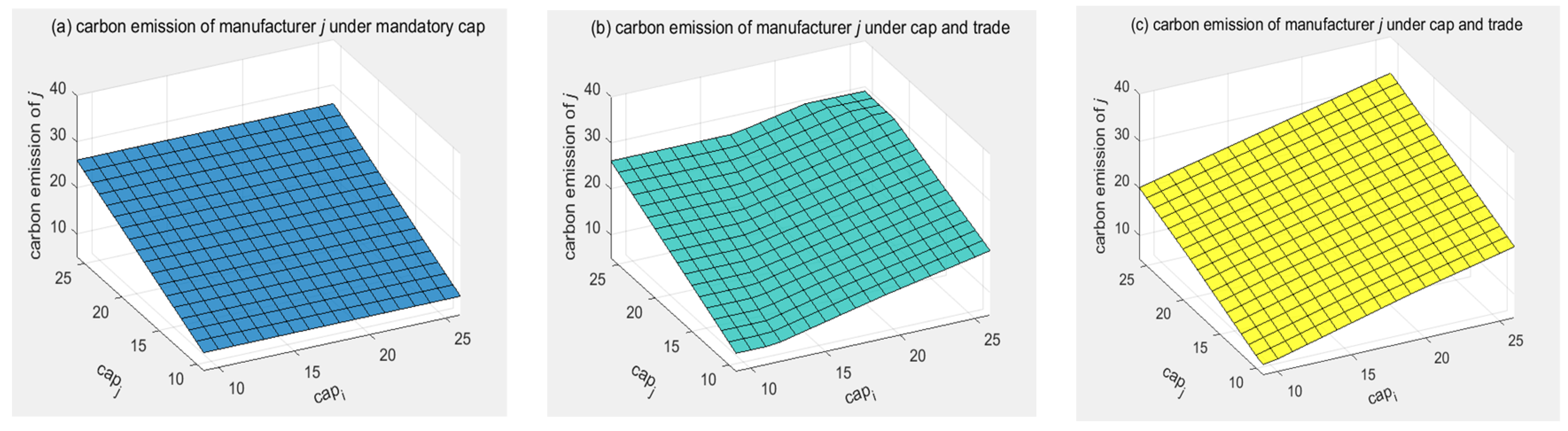
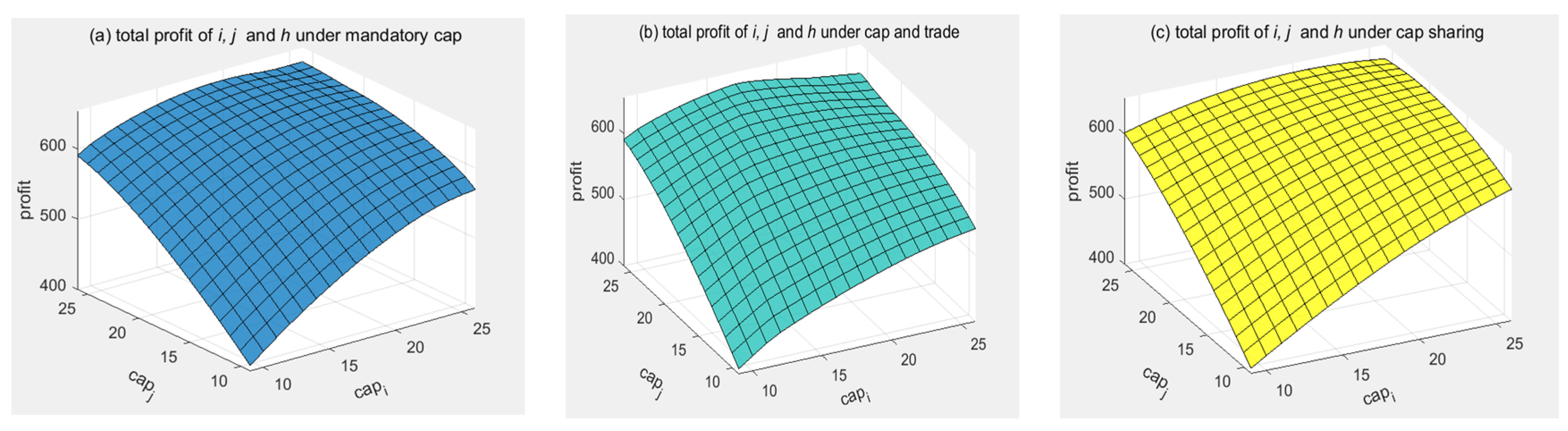
5.1. Analyzing the Effects of Cap on Optimal Decisions and Profits

We assume that $ca{p}_j$ and $ca{p}_i$ change from 9 to 26, respectively, then group the related equilibrium results into several matrixes corresponding to three carbon reduction regulations. We select data from the matrixes including the profits of manufacturers and recyclers and calculate the carbon emissions and the total profits of the supply chain based on the relevant data. The relevant results are illustrated in Figure 2, Figure 3, Figure 4, Figure 5, Figure 6 and Figure 7.

Figure 2 and Figure 4 illustrate the carbon emissions of two types of manufacturers under three carbon emission reduction regulations, respectively. Figure 3 and Figure 5 illustrate the profits of two types of manufacturers under three policies. Figure 6 and Figure 7 show the network performance.

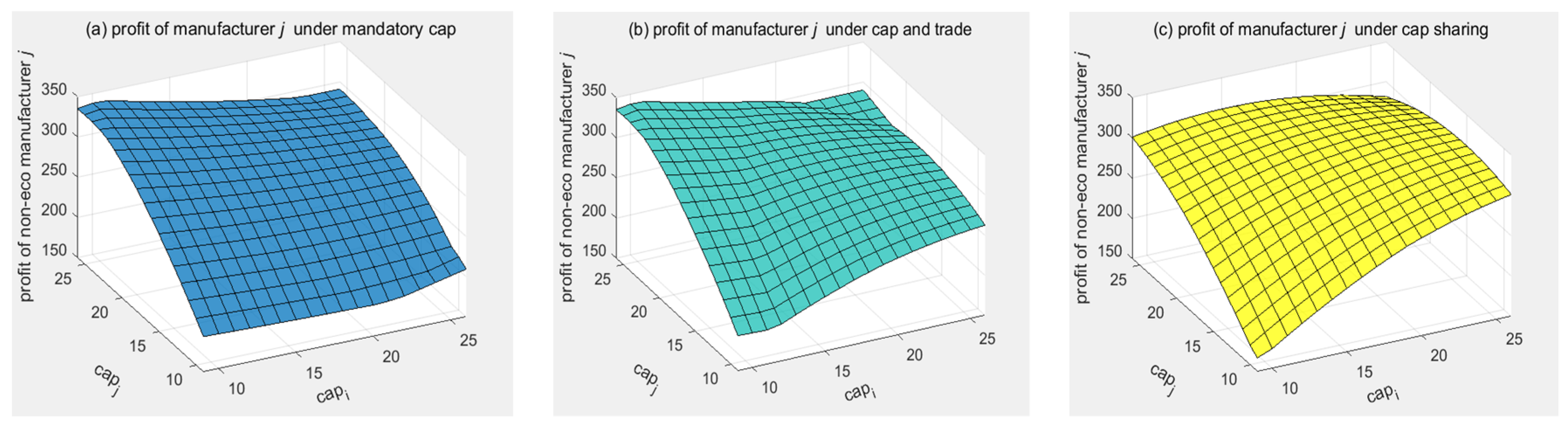
5.1.1. The Effects on Non-Ecological Manufacturer

As it can be seen from Figure 2, the trends are similar under the three regulations. Overall, the larger $ca{p}_j$ or $ca{p}_i$ incurs more carbon emissions. In Figure 2a, we can see that the carbon emission under MC is only affected by $ca{p}_j$, Figure 2b shows that the carbon emission under CT is greatly affected by $ca{p}_j$, and Figure 2c shows that the carbon emission under CS is affected by $ca{p}_j$ and $ca{p}_i$ simultaneously. The maximum value and minimum value appear in Figure 2c.

Comparing the three subfigures in Figure 2, the results show its carbon emissions and profits under policy MC are always lower than the other two policies, which means policy MC limits the enterprise’s production activity and injures its profit. However, there is a special interval: when $ca{p}_i$ is less than 14, policy CS is conductive to decrease carbon emissions because the lower cap cannot activate the recycling process. Policy CT and Constraint (6) are invalid. In addition, there is no cap trade between two manufacturers, manufacturers only use the allocated cap to produce, and policy MC and CT have the same effects on the equilibrium results.

When $ca{p}_i$ is larger than 14, policy CS and CT are valid. Under policy CS, carbon caps are transferred freely from eco manufacturers to non-eco manufacturers. When caps transaction exists, policy CT promotes the effective allocation of carbon caps and benefits social-economic development. The maximum profit appears in the region when $ca{p}_i$ is relatively small while $ca{p}_j$ is large under policy CT. This can be explained by the adequacy caps reducing its carbon trade activities.

In Figure 3, the trends are also similar under three regulations. The maximum values appear in Figure 3a,b, while the minimum value appears in Figure 3c. Figure 3a states that the profit is mainly affected by $ca{p}_j$ and is slightly affected by $ca{p}_i$. This phenomenon is different from carbon emissions. The reason can be explained by: the increasing caps will stimulate production activities, more customers turn to buy eco-products, and eco manufacturers’ profits increase. Figure 3c illustrates $ca{p}_j$ and $ca{p}_i$ have the same effects on non-eco manufacturers’ profit, and the profit is only influenced by caps.

The comparison of these three subfigures shows policy CT is a cost-effective carbon reduction policy. Particularly, when $ca{p}_i$ is lower, the profit in Figure 3b is similar to that in Figure 3a; when $ca{p}_i$ is higher, the profit in Figure 3b is similar to that in Figure 3c.

In addition, it should be noted that when $ca{p}_j$ and $ca{p}_i$ are large enough, the changing carbon emission trend is not exactly with that of the profit under policy CS, because the transportation cost increases rapidly with the intense production and recycling activities.

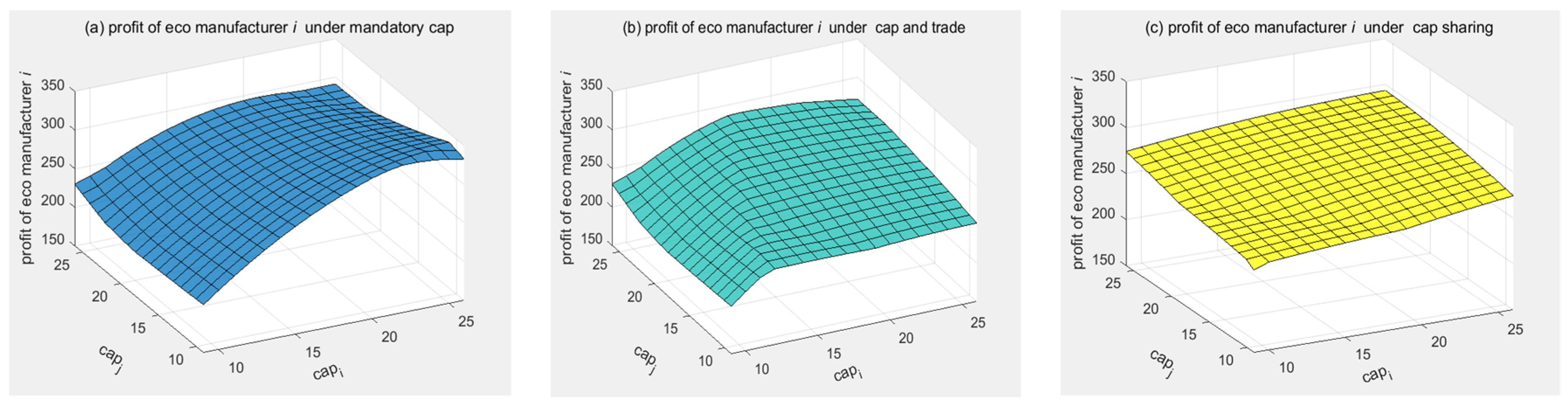
5.1.2. The Effects on Ecological Manufacturer

The analysis of eco manufacturers is similar to that of non-ecological manufacturers.

According to Figure 4, the equilibrium results of eco manufacturers are opposite to non-eco manufacturers in Figure 2. In Figure 4a, its carbon emission is only affected by $ca{p}_i$ in most ranges, which is similar to Figure 2a. In Figure 4b, when $ca{p}_i$ is at a relatively low level, it has no extra caps for sale, and policy CT is the same as MC. When $ca{p}_i$ gradually increases, the extra carbon quotas bring cap transactions. In Figure 4c, due to the adoption of ecological production technology, its carbon emission changes slightly.

Comparing the three subfigures of Figure 4, policy CS is the most effective method to reduce carbon emissions. Particularly, when $ca{p}_i$ is relatively small, carbon quotas are not transferred from eco manufacturers to non-eco manufacturers. Combined with Figure 5b, the carbon emissions and profits are identical under policy MC and CT. Policy MC is always beneficial for the eco manufacturer to obtain higher profits when $ca{p}_i$ is large. This phenomenon occurs because carbon quotas are adequate for it to produce more products, while policy CT and CS may force carbon caps to transfer to non-eco manufacturers.

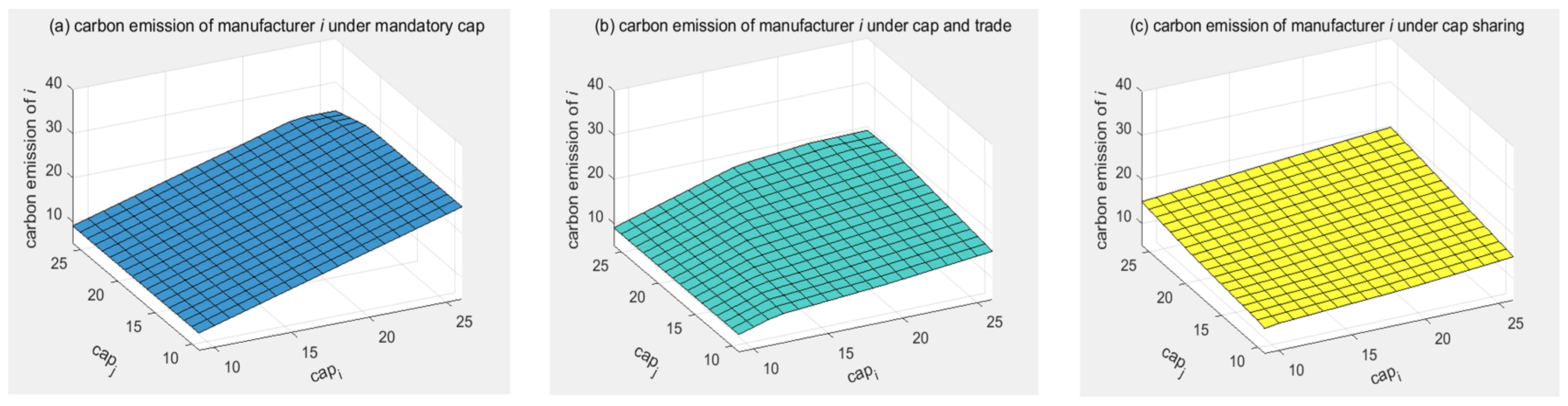
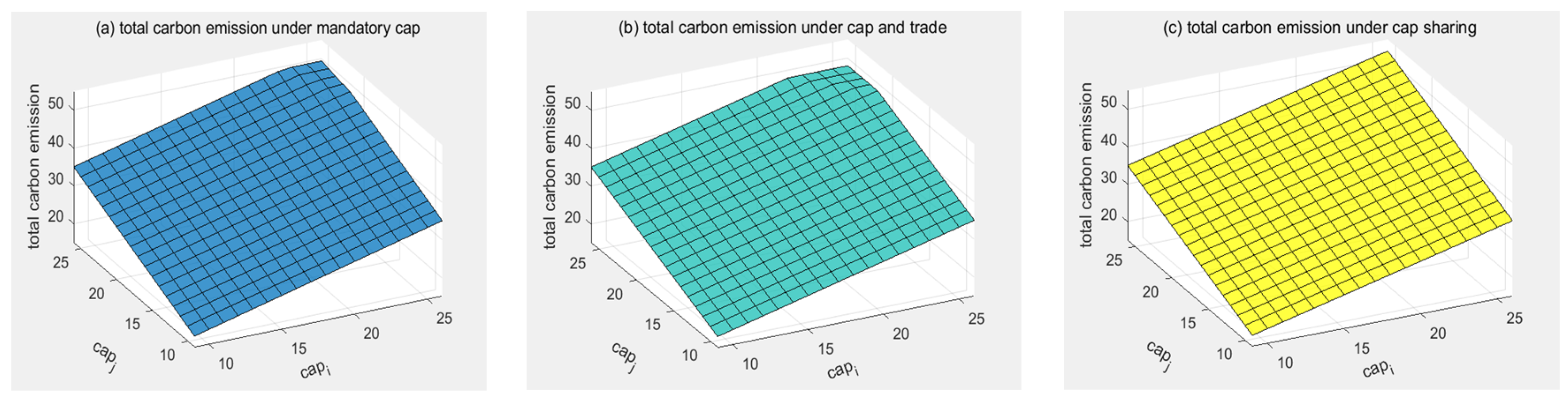
5.1.3. The Effects on Supply Chain Performance

In this subsection, we focus on the impact of different policies on the whole supply chain performance. Total carbon emission and profit are given in Figure 6. From the environmental perspective, total carbon emissions are equal in three scenarios. From the economic perspective, according to Figure 7, we can clearly see that the best policy is cap sharing, but the difference between each policy is small. Combined with the previous figures, when caps increase, policy CS also perform well in reducing manufacturers’ carbon emissions and promoting their profits. From the view of the government, the carbon trade model sacrifices part of the efficiency of the supply chain in exchange for government control and supervision of the carbon trading market. Although policy CS is an ideal regulation, if it lowers the carbon trade cost, policy CT may have a similar performance to policy CS, which makes it easier for the government to achieve the emissions reduction target.

Policy CT is conducive to the government to control the carbon emissions of enterprises; at the same time, the government may permit cap sharing within a large enterprise when there are different levels of low carbon technology applied in production.

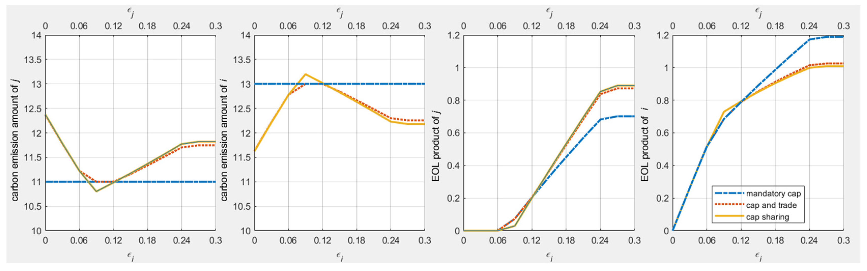
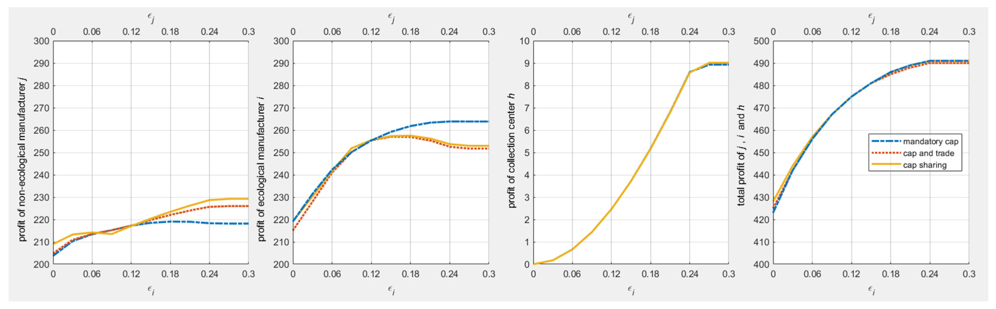
5.2. Analyzing Effects of ${\epsilon }_j$ and ${\epsilon }_i$ on Optimal Decisions and Profits

Figure 8 illustrates the impacts of parameter ${\epsilon }_j$ and ${\epsilon }_i$ in the interval [0, 0.3] on carbon emission amount and EOL product quantity, while Figure 9 shows the impacts on decision-makers’ profits.

From Figure 8, we can see that manufacturers’ carbon emission curves remain unchanged in policy MC. In policy CT and CS, manufacturer $j$’s carbon emission curve almost decreases, then increases, and finally stays invariant, while manufacturer $i$’s curve has an opposite trend, and ${\epsilon }_i={\epsilon }_j=0.09$ is the turning point. The observed phenomenon can be explained in the following manner. From the equilibrium decision value, we can see that the use of raw materials has been in a downward trend; thus, the emissions from raw materials continue to decrease. At first, non-eco manufacturer $j$’s carbon emissions are higher due to the higher unit emission factor. For EOL products, the point at which manufacturer $i$ begins to have EOL is 0, while the point at which manufacturer $j$ begins to have EOL is 0.6. Therefore, the carbon emissions of $j$ decreases at the beginning, and when ${\epsilon }_i={\epsilon }_j=0.09$, carbon emissions are minimum. After this point, the emission increased by the production and transportation of EOL remanufacturing is higher than the decrease in raw materials, and the emissions increase again. For eco manufacturer $i$, the same explanation can be made.

As for EOL product quantity, it is worth noting that when ${\epsilon }_i={\epsilon }_j>0$, the manufacturer $i$’s EOL product quantity increases gradually, when ${\epsilon }_j$ and ${\epsilon }_i$ are in the interval (0.06,0.09), the manufacturer $j$’s EOL product quantity becomes positive, and there is a turning point at 0.09 for manufacturer $i$ under policy CS. When ${\epsilon }_i={\epsilon }_j>0.24$, these curves in three scenarios gradually stabilize. In this scenario, Constraint (6) does not hold, which means that the collection center is unable to recycle at a specified proportion.

According to Figure 9, manufacturer $i$ always obtains more profit than manufacturer $j$. Overall, there is little difference in the total profits of the three cases; in particular, the total profits of all decision-makers in the policy CS are always higher than that in the other two cases. As for the collection center, the profit is almost the same under different regulations. For government, the recycling ratio should be set in an appropriate range. When it is too high, the enterprise will not comply with it, and it is meaningless. When the recycling ratio is set too low, it will fail to achieve the goal of resource utilization.

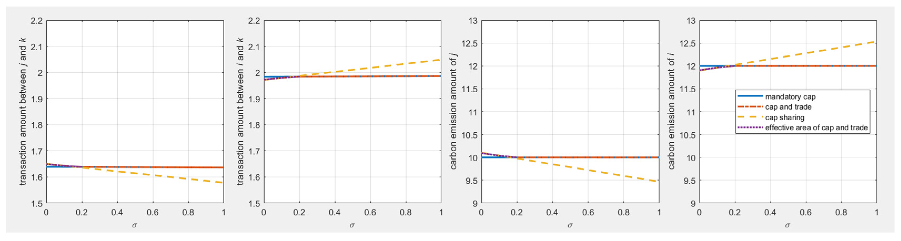
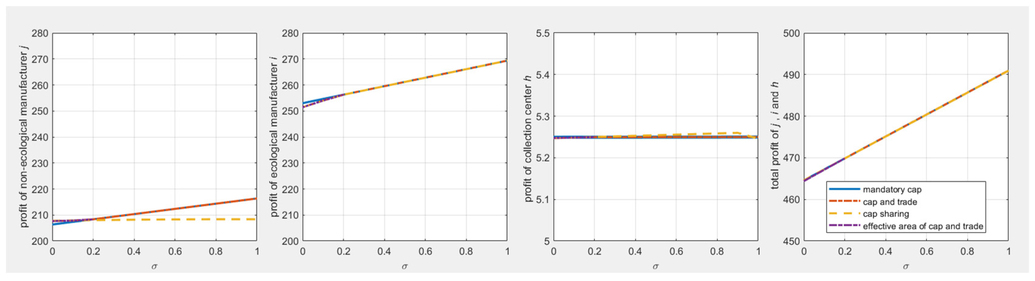
5.3. Analysis Effects of $\sigma$ on Optimal Decisions and Profits

Figure 10 illuminates the impacts of parameter $\sigma$ in the interval [0,1] on the product transaction amount and the carbon emissions amount, while Figure 11 shows the impacts on decision-makers’ profits.

In CS policy, increasing $\sigma$ has positive effects on the manufacturer $i$’s products transaction amount, whereas for manufacturer $j$, the situation is reversed. In the other two scenarios, the products transaction amounts stay unchanged. The carbon emission curve has a synchronous changing trend with the product transaction.

As can be seen from Figure 11, the profit of non-ecological manufacturer $j$ maintains stability in policy CS and increases a little in policy CT and MC. However, the profit of ecological manufacturer $i$ increases rapidly under the three regulations. The change in profits shows that this situation is more favorable to ecological manufacturers. For the total profit of the two types of manufacturers, there are almost no differences in these three cases. Similar to the analysis of previous examples, the profit of collection center $h$ is mainly affected by the EOL collection amount; thus, it maintains stability at first and decreases later. Therefore, the increasement of $\sigma$ will promote the development and impacts little on carbon emission.

5.4. Managerial Insights

Compared with the literature [3], this research highlights the difference between carbon emission reduction policies, and based on numerical examples and analysis, we present several managerial insights as follows. This may facilitate the government and enterprises to refer to when issuing policies and enterprises making operation decisions.

• Firstly, by comparing the three carbon emission policies, even though cap-and-trade regulations are more flexible than mandatory cap policy, it still loses a little efficiency than cap-sharing schemes. Both cap-and-trade regulations and cap-sharing schemes can encourage firms to adjust their production and pricing strategies. Governments should allocate caps properly and implement cap-sharing schemes in some pilot enterprises.
• Secondly, the proposed model proves that investment in green production technology helps ecological manufacturers gain lower carbon emissions and high profits. The technologies work both in forward and reverse channels. For wise enterprise leadership, correct decisions should be made on when and how to adopt cleaner production technology.
• Thirdly, the reverse supply chain should be valued at a strategic level because of its essential role in promoting a circular economy and sustainable development. Especially high-emission enterprises can complete green transformation and reduce emissions through recycling and remanufacturing processes.
• Finally, consumers are increasingly concerned about the impact of the production process on the environment. On the one hand, governments can reward manufacturers for producing more environmentally friendly products. On the other hand, the information or technology can be shared between enterprises.

6. Conclusions

In this paper, we expand the previous research to a CLSC network based on non-cooperative equilibrium. This paper provides a research framework for a series of Nash game problems of low-carbon supply chain networks with complex relationships between horizontal and vertical competitive members. The profit maximum problem with nonlinear constraints can be transformed into variational inequality, and the equilibrium results can be obtained through a modified projection and contraction algorithm.

In the forward flow, we suppose three different environmental regulations, namely mandatory cap, cap-and-trade, and cap sharing. The collection and remanufacturing of EOL products are taken into consideration in the reverse flow. The effects of policies on network performance are discussed in detail. The results show that:

(1)

Policy CS is effective in coordinating the relationship between economic development and environmental protection. In practice, the government may permit carbon cap sharing among enterprises, especially within a large enterprise to achieve a win-win situation. In other situations, CS policy may act as the ideal goal to measure the performance of MC and CT regulations.

(2)

Policy MC is easy to implement for governments, and the carbon reduction goal can be reached either. However, the carbon quotas cannot be converted to revenue, even if there are excess quotas for manufacturers.

(3)

Additionally, policy CT may lose a little efficiency compared with cap-sharing schemes, but it benefits government regulations. If governments can adjust cap transaction costs or relax carbon quotas, policy CT may show better performance. Moreover, policy CT can promote manufacturers adopting green technology to reduce carbon emissions, and the carbon emission rights have the nature of assets and create extra revenue.

(4)

It should be noted that in all scenarios, ecological manufacturers always show better performances, which means the green technology innovation can benefit firms both in sustainable development and economic development.

(5)

Consumers’ environmental protection awareness has a positive effect on ecological manufacturers but hurts non-eco manufacturers, especially in cap-sharing schemes. Moreover, when the recycling rate is at a relatively high level, it effectively helps eco manufacturers to use more reusable materials and reduce carbon emissions, whereas when it exceeds a certain value, the change has almost no influence on equilibrium results.

This study mainly contributes to the enterprises’ decision making and revenue management under three carbon emissions reduction regulations. Through numerical simulations, we verified the validity of each policy. For future research, possible extensions can be as follows:

(1)

Information sharing can be considered, especially the production cost for different manufacturers.

(2)

The model can include irrational behavior factors of decision-makers, such as free-riding behavior.

(3)

The online transaction fashion can be incorporated into the model, especially in the post-COVID-19 era.

(4)

Some practical constraints, such as financial constraints and capacity constraints, can be considered in the model in future research.

References

- Liu, P.T.; Liu, L.Y.; Xu, X. Carbon footprint and carbon emission intensity of grassland wind farms in Inner Mongolia. J. Clean. Prod. 2021, 313, 127878. [Google Scholar] [CrossRef]
- Liu, M.L.; Li, Z.H.; Anwar, S. Supply chain carbon emission reductions and coordination when consumers have a strong preference for low-carbon products. Environ. Sci. Pollut. Res. 2021, 28, 19969–19983. [Google Scholar] [CrossRef] [PubMed]
- Cheng, P.Y.; Ji, G.X.; Zhang, G.T. A closed-loop supply chain network considering consumer’s low carbon preference and carbon tax under the cap-and-trade regulation. Sustain. Prod. Consum. 2022, 29, 614–635. [Google Scholar] [CrossRef]
- Zhang, G.T.; Cheng, P.Y.; Sun, H. Carbon reduction decisions under progressive carbon tax regulations: A new dual-channel supply chain network equilibrium model. Sustain. Prod. Consum. 2021, 27, 1077–1092. [Google Scholar] [CrossRef]
- Yu, M.; Cruz, J.M.; Li, M.D. The sustainable supply chain network competition with environmental tax policies. Int. J. Prod. Econ. 2019, 217, 218–231. [Google Scholar] [CrossRef]
- Guchhait, R.; Sakar, B. Economic and environmental assessment of an unreliable supply chain management. RAIRO-Oper. Res. 2021, 55, 3153–3170. [Google Scholar] [CrossRef]
- Xu, X.F.; He, Y.Y. Blockchain application in modern logistics information sharing: A review and case study analysis. Prod. Plan. Control 2022, 1–15. [Google Scholar] [CrossRef]
- Zhang, W.; Yan, S.; Li, J. Credit risk prediction of SMEs in supply chain finance by fusing demographic and behavioral data. Transport. Res. E Logist. Transport. Rev. 2022, 158, 102611. [Google Scholar] [CrossRef]
- Guchhait, R.; Pareek, S.; Sakar, B. How Does a Radio Frequency Identification Optimize the Profit in an Unreliable Supply Chain Management? Mathematics 2019, 7, 490. [Google Scholar] [CrossRef] [Green Version]
- Wu, Y.S.; Lu, R.H.; Yang, J. Government-led low carbon incentive model of the online shopping supply chain considering the O2O model. J. Clean. Prod. 2021, 279, 123271. [Google Scholar] [CrossRef]
- He, L.; Hu, C.; Zhao, D. Carbon emission mitigation through regulatory policies and operations adaptation in supply chains: Theoretic developments and extensions. Nat. Hazards 2016, 84, 179–207. [Google Scholar] [CrossRef]
- Dinan, T. Policy Options for Reducing CO2 Emissions; Congress of the U.S. Congressional Budget Office: Washington, DC, USA, 2008.
- Yu, Y.G.; Zhou, S.J.; Shi, Y. Information sharing or not across the supply chain: The role of carbon emission reduction. Transport. Res. E Logist. Transport. Rev. 2020, 137, 101915. [Google Scholar] [CrossRef]
- Xu, X.F.; Wang, C.L.; Zhou, P. GVRP considered oil-gas recovery in refined oil distribution: From an environmental perspective. Int. J. Prod. Econ. 2021, 235, 108078. [Google Scholar] [CrossRef]
- Cao, J.; Chen, X.H.; Zhang, X.M. Overview of remanufacturing industry in China: Government policies, enterprise, and public awareness. J. Clean. Prod. 2020, 242, 1–17. [Google Scholar] [CrossRef]
- Cai, J.Y.; Cai, Z. Renewable resource industry’s international experience and enlightenment. Econ. Geogr. 2010, 30, 2044–2049. [Google Scholar]
- Xing, E.F.; Shi, C.D.; Zhang, J.X. Double third-party recycling closed-loop supply chain decision under the perspective of carbon trading. J. Clean. Prod. 2020, 259, 1–11. [Google Scholar] [CrossRef]
- Patel, G.S. A Stochastic Production Cost Model for Remanufacturing Systems. Master’s Thesis, The University of Texas-Pan American, Edinburg, TX, USA, 2006. [Google Scholar]
- Gregorio, R.S.; Sofía, E.M.; Carlos, R.A. Multivariable Supplier Segmentation in Sustainable Supply Chain Management. Sustainability 2020, 12, 4556. [Google Scholar]
- Zhang, X.X.; Ji, Y.N.; Shen, C.L. Manufacturers’ green investment in a competitive market with a common retailer. J. Clean. Prod. 2020, 276, 123164. [Google Scholar] [CrossRef]
- Guo, S.; Choi, T.M.; Shen, B. Green product development under competition: A study of the fashion apparel industry. Eur. J. Oper. Res. 2020, 280, 523–538. [Google Scholar] [CrossRef]
- Savaskan, R.C.; Bhattacharya, S.; Van Wassenhove, L.N. Closed-loop supply chain models with product remanufacturing. Manag. Sci. 2004, 50, 239–252. [Google Scholar] [CrossRef] [Green Version]
- Chen, C.K.; Ulya, M.A. Analyses of the reward-penalty mechanism in green closed-loop supply chains with product remanufacturing. Int. J. Prod. Econ. 2019, 210, 211–223. [Google Scholar] [CrossRef]
- Taleizadeh, A.A.; Alizadeh-Basban, N.; Niaki, S.T.A. A closed-loop supply chain considering carbon reduction, quality improvement effort, and return policy under two remanufacturing scenarios. J. Clean. Prod. 2019, 232, 1230–1250. [Google Scholar] [CrossRef]
- Yang, Y.; Xu, X. A differential game model for closed-loop supply chain participants under carbon emission permits. Comput. Ind. Eng. 2019, 135, 1077–1090. [Google Scholar] [CrossRef]
- Taleizadeh, A.A.; Moshtagh, M.S.; Moon, I. Optimal decisions of price, quality, effort level and return policy in a three-level closed-loop supply chain based on different game theory approaches. Eur. J. Int. Eng. 2017, 11, 486–525. [Google Scholar] [CrossRef] [Green Version]
- Zerang, E.S.; Taleizadeh, A.A.; Razmj, J. Analytical comparisons in a three-echelon closed-loop supply chain with price and marketing effort-dependent demand: Game theory approaches. Environ. Dev. Sustain. 2018, 20, 451–478. [Google Scholar] [CrossRef]
- Chu, J.F.; Shao, C.F.; Ali, E. Performance evaluation of organizations considering economic incentives for emission reduction: A carbon emission permit trading approach. Energy Econ. 2021, 101, 105398. [Google Scholar] [CrossRef]
- Wang, Y.J.; Chen, W.D.; Liu, B.Y. Manufacturing/remanufacturing decisions for a capital-constrained manufacturer considering carbon emission cap and trade. J. Prod. Clean. 2017, 140, 1118–1128. [Google Scholar] [CrossRef]
- Xu, L.; Wang, C. Sustainable manufacturing in a closed-loop supply chain considering emission reduction and remanufacturing. Resour. Conserv. Recycl. 2018, 131, 297–304. [Google Scholar] [CrossRef]
- Wang, C.; Miao, Z.; Chen, X. Factors affecting changes of greenhouse gas emissions in belt and road countries. Renew. Sust. Energ. Rev. 2021, 147, 111220. [Google Scholar] [CrossRef]
- Zhu, Q.; Li, X.; Li, F. Analyzing the sustainability of China’s industrial sectors: A data-driven approach with total energy consumption constraint. Ecol. Indic. 2021, 122, 107235. [Google Scholar] [CrossRef]
- Chai, Q.F.; Xiao, Z.D.; Lai, K.H. Can carbon cap and trade mechanism be beneficial for remanufacturing? Int. J. Prod. Econ. 2018, 203, 311–321. [Google Scholar] [CrossRef]
- Si, M.X.; Bai, L.; Du, K. Fuel consumption analysis and cap and trade system evaluation for Canadian in situ oil sands extraction. Renew. Sustain. Energy Rev. 2021, 146, 111145. [Google Scholar] [CrossRef]
- Ji, J.N.; Zhang, Z.Y.; Yang, L. Comparisons of initial carbon allowance allocation rules in an O2O retail supply chain with the cap-and-trade regulation. Int. J. Prod. Econ. 2017, 187, 68–84. [Google Scholar] [CrossRef]
- Zhang, B.; Xu, L. Multi-item production planning with carbon cap and trade mechanism. Int. J. Prod. Econ. 2013, 144, 118–127. [Google Scholar] [CrossRef]
- Du, S.; Ma, F.; Fu, Z. Game-theoretic analysis for an emission-dependent supply chain in a ‘cap-and-trade’ system. Ann. Oper. Res. 2015, 228, 135–149. [Google Scholar] [CrossRef]
- Yang, G.F.; Wang, Z.P.; Li, X.Q. The optimization of the closed-loop supply chain network. Transport. Res. E Logist. Transport. Rev. 2008, 45, 16–28. [Google Scholar] [CrossRef]
- Xu, X.F.; He, J.; Zheng, Y. Multi-objective artificial bee colony algorithm for multi-stage resource leveling problem in sharing logistics network. Comput. Ind. Eng. 2020, 142, 106338. [Google Scholar] [CrossRef]
- Nagurney, A.; Dong, J.; Zhang, D. A supply chain network equilibrium model. Transp. Res. Part E Logist. Transp. Rev. 2002, 38, 281–303. [Google Scholar] [CrossRef]
- Nagurney, A.; Daniele, P.; Shukla, S. A supply chain network game theory model of cybersecurity investments with nonlinear budget constraints. Ann. Oper. Res. 2017, 248, 405–427. [Google Scholar] [CrossRef]
- Nagurney, A.; Yu, M. Sustainable fashion supply chain management under oligopolistic competition and brand differentiation. Int. J. Prod. Econ. 2012, 135, 532–540. [Google Scholar] [CrossRef]
- He, L.F.; Xu, Z.G.; Niu, Z.W. Joint optimal production planning for complex supply chains constrained by carbon emission abatement policies. Discrete Dyn. Nat. Soc. 2014, 2014, 361923. [Google Scholar] [CrossRef]
- Tao, Z.G.; Zhong, Y.G.; Sun, H. Multi-period closed-loop supply chain network equilibrium with carbon emission constrains. Resour. Conserv. Recycl. 2015, 104, 354–365. [Google Scholar] [CrossRef]
- He, L.F.; Mao, J.; Hu, C.L. Carbon emission regulation and operations in the supply chain network under stringent carbon policy. J. Clean. Prod. 2019, 238, 1–18. [Google Scholar] [CrossRef]
- Li, Q.; Long, R.; Chen, H. Empirical study of the willingness of consumers to purchase low-carbon products by considering carbon labels: A case study. J. Clean. Prod. 2017, 161, 1237–1250. [Google Scholar] [CrossRef]
- Hong, Z.; Wang, H.; Yu, Y. Green product pricing with non-green product reference. Transp. Res. Part E Logist. Transp. Rev. 2018, 115, 1–15. [Google Scholar] [CrossRef]
- Ma, S.G.; He, Y.; Gu, R.; Li, S.S. Sustainable supply chain management considering technology investments and government intervention. Transp. Res. Part E Logist. Transp. Rev. 2021, 149, 102290. [Google Scholar] [CrossRef]
- Tong, W.; Mu, D.; Zhao, F. The impact of cap-and-trade mechanism and consumers’ environmental preferences on a retailer-led supply chain. Resour. Conserv. Recycl. 2019, 142, 88–100. [Google Scholar] [CrossRef]
- Allevi, E.; Gnudi, A.; Konnov, I.V. Evaluating the effect of environmental regulations on a closed-loop supply chain network: A variational inequality approach. Ecol. Environ. Conserv. 2018, 261, 1–43. [Google Scholar] [CrossRef]
- Gao, J.; Han, H.; Hou, L. Pricing and effort decisions in a closed-loop supply chain under different channel power structures. J. Clean. Prod. 2016, 112, 2043–2205. [Google Scholar] [CrossRef]
- Hong, X.; Govindan, K.; Xu, L. Quantity and collection decisions in a closed-loop supply chain with technology licensing. Eur. J. Oper. Res. 2017, 3, 820–829. [Google Scholar] [CrossRef]
- Huang, Y.; Wang, Z. Values of information sharing: A comparison of supplier-remanufacturing and manufacturer-remanufacturing scenarios. Transport. Res. Part E 2017, 106, 20–44. [Google Scholar] [CrossRef]
- Huang, Y.; Wang, Z. Closed-loop supply chain models with product take-back and hybrid remanufacturing under technology licensing. J. Clean. Prod. 2017, 142, 3917–3927. [Google Scholar] [CrossRef]
- Liao, Z.; Zhu, X.; Shi, J. Case study on initial allocation of Shanghai carbon emission trading based on Shapley value. J. Clean. Prod. 2015, 103, 338–344. [Google Scholar] [CrossRef]
- Ray, S.; Jewkes, E.M. Customer lead time management when both demand and price are lead time sensitive. Eur. J. Oper. Res. 2004, 153, 769–781. [Google Scholar] [CrossRef]
- Liu, Z.G.; Anderson, T.D.; Cruz, J.M. Consumer environmental awareness and competition in two-stage supply chains. Eur. J. Oper. Res. 2012, 218, 602–613. [Google Scholar] [CrossRef]
- Hammond, D.; Beullens, P. Closed-loop supply chain network equilibrium under legislation. Eur. J. Oper. Res. 2007, 183, 895–908. [Google Scholar] [CrossRef]
- Paksoy, T.; Özceylan, E.; Weber, G.W. A multi objective model for optimization of a green supply chain network. Glob. J. Technol. Optim. 2011, 2, 84–96. [Google Scholar] [CrossRef]
- Cheng, F.L.; Sue, J.L.; Charles, L. Analysis of the impacts of combining carbon taxation and emission trading on different industry sectors. Energy Policy 2008, 36, 722–729. [Google Scholar]
- Kinderlehrer, D.; Stampacchia, G. An Introduction to Variational Inequalities and their Applications; Society for Industrial Mathematics: Philadelphia, PA, USA, 1987. [Google Scholar]