
Projecting Mortality Rates Using a Markov Chain


Abstract
1. Introduction
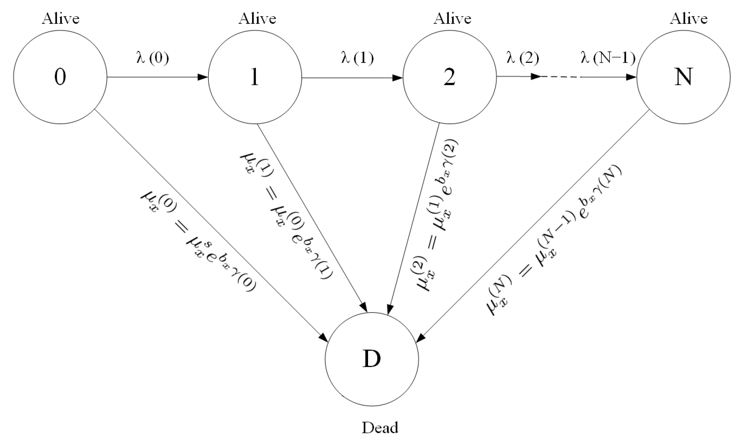
2. The Model
3. Mortality Data
4. Model Calibration to Mortality Data
4.1. Outline of Calibration Procedure
4.2. Preliminary Model without Age Effects
4.3. Full Model with Age Effects
4.4. Results of Calibration
5. Forecasting
5.1. Forecasting Procedure
5.2. Forecast Accuracy
6. Applications in Life Insurance and Pensions
7. Conclusions
Author Contributions
Funding
Institutional Review Board Statement
Informed Consent Statement
Data Availability Statement
Conflicts of Interest
Appendix A. Innovations State Space Model

| Y | N | cAIC | ||||||
|---|---|---|---|---|---|---|---|---|
| 1950 | 50 | 0.9983 | 0.9983 | 1 | 39.55 | 0.2439 | 61.69 | |
| 1990 | 10 | 0.0001 | 0.0001 | 1 | 4.4896 | 0.3163 | 18.08 |
References
- Lee, R.D.; Carter, L.R. Modeling and forecasting US mortality. J. Am. Stat. Assoc. 1992, 87, 659–671. [Google Scholar] [CrossRef]
- Cairns, A.J.G.; Blake, D.; Dowd, K.; Coughlan, G.D.; Epstein, D.; Ong, A.; Balevich, I. A quantitative comparison of stochastic mortality models using data from England and Wales and the United States. N. Am. Actuar. J. 2009, 13, 1–35. [Google Scholar] [CrossRef]
- Cairns, A.J.G.; Blake, D.; Dowd, K.; Coughlan, G.D.; Epstein, D.; Khalaf-Allah, M. Mortality density forecasts: An analysis of six stochastic mortality models. Insur. Math. Econ. 2011, 48, 355–367. [Google Scholar] [CrossRef]
- Dowd, K.; Cairns, A.J.G.; Blake, D.; Coughlan, G.D.; Epstein, D.; Khalaf-Allah, M. Evaluating the goodness of fit of stochastic mortality models. Insur. Math. Econ. 2010, 47, 255–265. [Google Scholar] [CrossRef]
- Dowd, K.; Cairns, A.J.G.; Blake, D.; Coughlan, G.D.; Epstein, D.; Khalaf-Allah, M. Backtesting stochastic mortality models: An ex post evaluation of multiperiod-ahead density forecasts. N. Am. Actuar. J. 2010, 14, 281–298. [Google Scholar] [CrossRef]
- Haberman, S.; Renshaw, A.E. A comparative study of parametric mortality projection models. Insur. Math. Econ. 2011, 48, 35–55. [Google Scholar] [CrossRef]
- Stoeldraijer, L.; Van Duin, C.; Van Wissen, L.; Janssen, F. Impact of different mortality forecasting methods and explicit assumptions on projected future life expectancy: The case of the Netherlands. Demogr. Res. 2013, 29, 323–354. [Google Scholar] [CrossRef]
- Guibert, Q.; Lopez, O.; Piette, P. Forecasting mortality rate improvements with a high-dimensional VAR. Insur. Math. Econ. 2019, 88, 255–272. [Google Scholar] [CrossRef]
- Hunt, A.; Blake, D. On the structure and classification of mortality models. N. Am. Actuar. J. 2021, 25, S215–S234. [Google Scholar] [CrossRef]
- Booth, H.; Tickle, L. Mortality modelling and forecasting: A review of methods. Ann. Actuar. Sci. 2008, 3, 3–43. [Google Scholar] [CrossRef]
- Lee, R.; Miller, T. Evaluating the performance of the Lee-Carter method for forecasting mortality. Demography 2001, 38, 537–549. [Google Scholar] [CrossRef] [PubMed]
- Booth, H.; Maindonald, J.; Smith, L. Applying Lee-Carter under conditions of variable mortality decline. Popul. Stud. 2002, 56, 325–336. [Google Scholar] [CrossRef]
- Brouhns, N.; Denuit, M.; Vermunt, J.K. A Poisson log-bilinear regression approach to the construction of projected lifetables. Insur. Math. Econ. 2002, 31, 373–393. [Google Scholar] [CrossRef]
- Hatzopoulos, P.; Haberman, S. A parameterized approach to modeling and forecasting mortality. Insur. Math. Econ. 2009, 44, 103–123. [Google Scholar] [CrossRef]
- Hyndman, R.J.; Ullah, M.S. Robust forecasting of mortality and fertility rates: A functional data approach. Comput. Stat. Data Anal. 2007, 51, 4942–4956. [Google Scholar] [CrossRef]
- De Jong, P.; Tickle, L. Extending Lee–Carter mortality forecasting. Math. Popul. Stud. 2006, 13, 1–18. [Google Scholar] [CrossRef]
- Booth, H.; Hyndman, R.J.; Tickle, L.; De Jong, P. Lee-Carter mortality forecasting: A multi-country comparison of variants and extensions. Demogr. Res. 2006, 15, 289–310. [Google Scholar] [CrossRef]
- Cairns, A.J.G.; Blake, D.; Dowd, K. A two-factor model for stochastic mortality with parameter uncertainty: Theory and calibration. J. Risk Insur. 2006, 73, 687–718. [Google Scholar] [CrossRef]
- Li, H.; O’Hare, C. Semi-parametric extensions of the Cairns–Blake–Dowd model: A one-dimensional kernel smoothing approach. Insur. Math. Econ. 2017, 77, 166–176. [Google Scholar] [CrossRef]
- Renshaw, A.E.; Haberman, S. A cohort-based extension to the Lee–Carter model for mortality reduction factors. Insur. Math. Econ. 2006, 38, 556–570. [Google Scholar] [CrossRef]
- Plat, R. On stochastic mortality modeling. Insur. Math. Econ. 2009, 45, 393–404. [Google Scholar] [CrossRef]
- Cairns, A.J.G.; Blake, D.; Dowd, K.; Coughlan, G.D.; Khalaf-Allah, M. Bayesian stochastic mortality modelling for two populations. ASTIN Bull. J. IAA 2011, 41, 29–59. [Google Scholar] [CrossRef]
- Reither, E.N.; Olshansky, S.J.; Yang, Y. New forecasting methodology indicates more disease and earlier mortality ahead for today’s younger Americans. Health Aff. 2011, 30, 1562–1568. [Google Scholar] [CrossRef][Green Version]
- Levantesi, S.; Pizzorusso, V. Application of machine learning to mortality modeling and forecasting. Risks 2019, 7, 26. [Google Scholar] [CrossRef]
- Atance, D.; Debón, A.; Navarro, E. A comparison of forecasting mortality models using resampling methods. Mathematics 2020, 8, 1550. [Google Scholar] [CrossRef]
- Norberg, R. Optimal hedging of demographic risk in life insurance. Financ. Stochastics 2013, 17, 197–222. [Google Scholar] [CrossRef]
- Lin, X.S.; Liu, X. Markov aging process and phase-type law of mortality. N. Am. Actuar. J. 2007, 11, 92–109. [Google Scholar] [CrossRef]
- Liu, X.; Lin, X.S. A subordinated Markov model for stochastic mortality. Eur. Actuar. J. 2012, 2, 105–127. [Google Scholar] [CrossRef]
- Dickson, D.C.M.; Hardy, M.R.; Waters, H.R. Actuarial Mathematics for Life Contingent Risks, 2nd ed.; Cambridge University Press: New York, NY, USA, 2013. [Google Scholar]
- Hyndman, R.J.; Koehler, A.B.; Ord, J.K.; Snyder, R.D. Forecasting with Exponential Smoothing: The State Space Approach; Springer: Berlin/Heidelberg, Germany, 2008. [Google Scholar]
- Amsler, M.H. Les chaines de Markov des assurances vie, invalidité et maladie. In Proceedings of the Transactions of the 18th International Congress of Actuaries, Munich, Germany, 4–11 June 1968; Volume 5, pp. 731–746. [Google Scholar]
- Hoem, J.M. Markov chain models in life insurance. Blätter Der DGVFM 1969, 9, 91–107. [Google Scholar] [CrossRef]
- Haberman, S.; Pitacco, E. Actuarial Models for Disability Insurance; Chapman & Hall: London, UK, 2018. [Google Scholar]
- Wolthuis, H. Life Insurance Mathematics (The Markovian Model); IAE, Universiteit van Amsterdam: Amsterdam, The Netherlands, 2003. [Google Scholar]
- Chiou, J.M.; Müller, H.G. Modeling hazard rates as functional data for the analysis of cohort lifetables and mortality forecasting. J. Am. Stat. Assoc. 2009, 104, 572–585. [Google Scholar] [CrossRef]
- Human Mortality Database. 2020. Available online: https://www.mortality.org/ (accessed on 5 March 2020).
- Jarner, S.F.; Kryger, E.M. Modelling adult mortality in small populations: The SAINT model. ASTIN Bull. 2011, 41, 377–418. [Google Scholar] [CrossRef]
- Itô, K. Encyclopedic Dictionary of Mathematics, 2nd ed.; MIT Press: Cambridge, MA, USA, 1993. [Google Scholar]
- Shreve, S.E. Stochastic Calculus for Finance II: Continuous-Time Models; Springer: New York, NY, USA, 2004; Volume 11. [Google Scholar]
- Pitacco, E.; Denuit, M.; Haberman, S.; Olivieri, A. Modelling Longevity Dynamics for Pensions and Annuity Business; Oxford University Press: New York, NY, USA, 2009. [Google Scholar]
- Benjamin, B.; Pollard, J.H. The Analysis of Mortality and Other Actuarial Statistics; The Institute of Actuaries: Oxford, UK, 1993; Volume 3. [Google Scholar]
- Johnson, C.R. Positive definite matrices. Am. Math. Mon. 1970, 77, 259–264. [Google Scholar] [CrossRef]
- Perlis, S. Theory of Matrices; Addison-Wesley: Reading, MA, USA, 1952. [Google Scholar]
- CMIB. Report no. 17 Continuous Mortality Investigation Bureau; Technical Report; Institute and Faculty of Actuaries: London, UK, 1999. [Google Scholar]
- Hyndman, R.J.; Koehler, A.B.; Snyder, R.D.; Grose, S. A state space framework for automatic forecasting using exponential smoothing methods. Int. J. Forecast. 2002, 18, 439–454. [Google Scholar] [CrossRef]
- Ord, J.K.; Koehler, A.B.; Snyder, R.D. Estimation and prediction for a class of dynamic nonlinear statistical models. J. Am. Stat. Assoc. 1997, 92, 1621–1629. [Google Scholar] [CrossRef]
- McKenzie, E.; Gardner, E.S. Damped trend exponential smoothing: A modelling viewpoint. Int. J. Forecast. 2010, 26, 661–665. [Google Scholar] [CrossRef]
- Makridakis, S.; Hibon, M. The M3-Competition: Results, conclusions and implications. Int. J. Forecast. 2000, 16, 451–476. [Google Scholar] [CrossRef]
- Gardner, E.S.; McKenzie, E. Why the damped trend works. J. Oper. Res. Soc. 2011, 62, 1177–1180. [Google Scholar] [CrossRef]
- Fildes, R. The evaluation of extrapolative forecasting methods. Int. J. Forecast. 1992, 8, 81–98. [Google Scholar] [CrossRef]


| N | ||
|---|---|---|
| 25 | ||
| 50 | 1 | |
| 100 | 2 | |
| 150 | 3 | |
| 200 | 4 | |
| 300 | 6 | |
| 400 | 8 |
| State k | State k | State k | |||
|---|---|---|---|---|---|
| 0 | 17 | 34 | |||
| 1 | 18 | 35 | |||
| 2 | 19 | 36 | |||
| 3 | 20 | 37 | |||
| 4 | 21 | 38 | |||
| 5 | 22 | 39 | |||
| 6 | 23 | 40 | |||
| 7 | 24 | 41 | |||
| 8 | 25 | 42 | |||
| 9 | 26 | 43 | |||
| 10 | 27 | 44 | |||
| 11 | 28 | 45 | |||
| 12 | 29 | 46 | |||
| 13 | 30 | 47 | |||
| 14 | 31 | 48 | |||
| 15 | 32 | 49 | |||
| 16 | 33 | 50 |
| Age x | Age x | Age x | Age x | ||||
|---|---|---|---|---|---|---|---|
| 20 | 42 | 64 | 86 | ||||
| 21 | 43 | 65 | 87 | ||||
| 22 | 44 | 66 | 88 | ||||
| 23 | 45 | 67 | 89 | ||||
| 24 | 46 | 68 | 90 | ||||
| 25 | 47 | 69 | 91 | ||||
| 26 | 48 | 70 | 92 | ||||
| 27 | 49 | 71 | 93 | ||||
| 28 | 50 | 72 | 94 | ||||
| 29 | 51 | 73 | 95 | ||||
| 30 | 52 | 74 | 96 | ||||
| 31 | 53 | 75 | 97 | ||||
| 32 | 54 | 76 | 98 | ||||
| 33 | 55 | 77 | 99 | ||||
| 34 | 56 | 78 | 100 | ||||
| 35 | 57 | 79 | 101 | ||||
| 36 | 58 | 80 | 102 | ||||
| 37 | 59 | 81 | 103 | ||||
| 38 | 60 | 82 | 104 | ||||
| 39 | 61 | 83 | |||||
| 40 | 62 | 84 | |||||
| 41 | 63 | 85 |
| Year | Naïve | ||
|---|---|---|---|
| 2001 | 0.348 | 1.054 | 0.349 |
| 2002 | 0.341 | 1.150 | 0.299 |
| 2003 | 0.511 | 1.443 | 0.387 |
| 2004 | 0.743 | 1.718 | 0.545 |
| 2005 | 1.147 | 1.568 | 0.685 |
| 2006 | 1.530 | 2.013 | 0.955 |
| 2007 | 1.870 | 2.069 | 1.079 |
| 2008 | 1.761 | 2.427 | 0.992 |
| 2009 | 3.008 | 3.149 | 1.767 |
| 2010 | 3.641 | 2.972 | 1.927 |
| 2011 | 4.207 | 3.390 | 2.116 |
| 2012 | 4.985 | 2.868 | 2.412 |
| 2013 | 5.140 | 3.171 | 2.334 |
| 2014 | 5.421 | 3.701 | 2.269 |
| 2015 | 5.110 | 3.332 | 2.406 |
| 2016 | 4.642 | 3.574 | 2.192 |
| Total | 44.405 | 39.599 | 22.714 |
Publisher’s Note: MDPI stays neutral with regard to jurisdictional claims in published maps and institutional affiliations. |
© 2022 by the authors. Licensee MDPI, Basel, Switzerland. This article is an open access article distributed under the terms and conditions of the Creative Commons Attribution (CC BY) license (https://creativecommons.org/licenses/by/4.0/).
Share and Cite
Spreeuw, J.; Owadally, I.; Kashif, M. Projecting Mortality Rates Using a Markov Chain. Mathematics 2022, 10, 1162. https://doi.org/10.3390/math10071162
Spreeuw J, Owadally I, Kashif M. Projecting Mortality Rates Using a Markov Chain. Mathematics. 2022; 10(7):1162. https://doi.org/10.3390/math10071162
Chicago/Turabian StyleSpreeuw, Jaap, Iqbal Owadally, and Muhammad Kashif. 2022. "Projecting Mortality Rates Using a Markov Chain" Mathematics 10, no. 7: 1162. https://doi.org/10.3390/math10071162
APA StyleSpreeuw, J., Owadally, I., & Kashif, M. (2022). Projecting Mortality Rates Using a Markov Chain. Mathematics, 10(7), 1162. https://doi.org/10.3390/math10071162