Impact of Stratum Composition Changes on the Accuracy of the Estimates in a Sample Survey

Abstract

The study is devoted to measuring the impact of the element changes on the bias and variance of the estimator of the total in a sample business survey. Stratified simple random sampling is usually used in business surveys. Enterprises may join, split or change the stratum between sample selection and data collection. Assuming a model for enterprises joining and a model for the enterprises changing the stratum with some probability, expressions for the adjusted estimators of the total and the adjusted estimators of their variances are proposed. The influence of the enterprise changes on the variances of the estimators of the total is measured by the relative differences, i.e., by comparing them with the estimators, if there were no changes. The analytic results are illustrated with a simulation study using modified enterprise data. The simulation results demonstrate a large impact of the enterprise changes on the accuracy of the estimates, even in the case of the low probability of changes. The simulation results justify the need for adjustment of the enterprise changes between the sample selection and data collection, in order to improve the accuracy of results and the adjustment method available.

1. Introduction

The enterprise population is permanently changing. Its elements are economic units, and the indicators characterizing them may vary: main activity, composition (constitutive establishments), number of employees, and revenue. These changes are rather smooth during the periods of economic stability; however, they may become more drastic during the periods of economic growth or crises.

Table 1. Changes in GDP and number of employed persons in 19 countries of the euro area during COVID 19 pandemic.

	2019 Q4	2020 Q1	2020 Q2	2020 Q3	2020 Q4	2021 Q1	2021 Q2	2021 Q3
GDP relative change (%)	3.8	−7.8	−8.9	10.7	4.3	−4.7	4.5	2.8
Number of employed persons absolute change (mln)	0.4	−1.9	−3.0	1.7	0.7	−2.7	3.1	2.4

shows the changes in GDP and employment during the COVID-19 pandemic in the 19 countries of the euro area (Eurostat [1,2]). It shows that the relative percentage change in the gross domestic product on the previous period in the 1st quarter of 2020 equals −7.8, while it was positive in the 4th quarter of 2019 and earlier. Correspondingly, the number of employed persons in the 1st quarter of 2020 decreased by 1.9 million since 2019. Rapid changes in both directions are observed at later time periods: an increase in the number of employed persons and GDP in the 3rd and 4th quarter of 2020 and a repeated decrease in the 1st quarter of 2021. All these things point to the enterprise population changes.

Population changes influence the choice of statistical methods by the survey statisticians aiming to obtain survey results which would be as accurate as possible. The errors of statistical estimates in the sample surveys arise from many different sources: quality of the sampling frame, sampling itself, record linkage, data editing, adjustment for nonresponse, imputation, quality of auxiliary information, estimators used, etc.

Errors from different sources constitute the total survey error (TSE). A history of this concept is narrated by Lyberg et al. [3]. At the fountainhead of sample surveys, sampling design and its implementation (questionnaire effect, interviewer effect, nonresponse) were considered as the only available non-sampling sources of the survey error. Even industrial quality control methods were applied to reduce their influence on the survey results in some offices. Around 1970, it was still considered that all error sources can be taken into account when designing the survey. At the end of the 20th century, other aspects of survey errors appeared on the statisticians’ agenda. TSE is a statistical instrument aiming to cover the influence of all error sources on the quality of statistical results. Demographic events, such as enterprise birth, reactivation, death, merger, survival and many others are defined for the enterprises. They are deeply investigated for detailed classification and included in the Guidelines on the Use of Statistical Business Registers [4]. This shows the importance of the enterprise survival events for statistical purposes.

In connection with TSE, the participants of the European Establishment Statistics Workshop [5] introduce a concept of the “unit problem”, which addresses the situation when the survey from which the data are obtained differs from the element from which the data should be obtained, e.g., unit error. The main aspects of the unit error and the corresponding unit problem are summarised in [6] by Delden et al. The authors propose to include the unit errors in the total survey error framework. The unit problem means a unit error, which affects the quality of statistical results.

A question arose in [7], asking whether all statistics produced should include an estimate of the unit model error and show how the statistical output depends on various unit error models. It would be a large and complicated task, which could be performed only for a small number of case studies, because of the amount of effort required to define units and to distribute the collected data to them. It would not be possible to create a single measure for the unit error because of the diversity of errors. Sometimes, even the structure of the unit is not clear. Nevertheless, if a case study for the estimation of the unit error is conducted, it helps to understand the input of the unit error to the uncertainty of statistical results.

The current paper shares the opinion that only specific case studies can present situations in which the influence of the shortcomings of the statistical input on the quality of statistical results can be measured. We present some of the case studies into business surveys conducted by various statisticians in Section 2. Section 3 includes an introduction to survey sampling and stratified sampling design. It is followed by our own case study. It is devoted to measuring the impact of the unit errors on the bias and variance of the estimator of the total in a business survey, at a point when enterprises may join, split or change the stratum between sampling selection and data collection. First and second order inclusion probabilities are recalculated for the enterprises which have merged assuming a joining model. Expressions for the estimators of the stratum total and its variance are obtained in the case when enterprises change the stratum assuming a stratum change model. The statistical simulation results in Section 4 provide a numeric illustration and show big changes in variance estimates for the estimators of the totals due to enterprise population changes. The article ends with Results, Discussion and Appendix. This study has some intersection with the results included in the project report [8]. The results of the whole project on the quality for multisource statistics are shortly described in [9].

2. Overview of the Case Studies

The overview starts with the measurement errors and data editing, continues with the errors due to the inaccurate usage of the terms, and finally deals with the changes in the enterprise composition.

The knowledge of the effect of the data errors on the accuracy of statistics produced is also useful for the editing process, aimed at improving data quality. It is not possible for all data units to be edited manually because of the time limitations, costs, and quality requirements. De Waal et al. [10] developed selective editing methods. These methods aim at limiting manual editing by paying attention to the units with a high risk of errors essentially affecting the accuracy of statistical results.

In order to reduce the TSE, it was decided to consider that selective editing is an algorithm acting in two steps: finding the erroneous observations and minimizing the number of records going through manual editing. It means that some of the observations fail editing checks and still remain unadjusted. A Heckman model for these remaining observations is proposed by Laitila et al. [11]. According to this model, an observation may be without an error or may have an error satisfying the linear model. After estimating parameters for this model, expected values of the measurement errors can be estimated.

In order to clarify the essence of the following discussion, we have included the definitions of some of the concepts in the article (OECD, [12]). An enterprise is the smallest organisational union consisting of the legal units which produce goods or offers services. Legal units are economic units acting in their own right. An enterprise carries out its activities in several locations and consists of local units if there are more than one of them; alternatively, it is itself a local unit if there are no more compounding units. An establishment is a local unit dealing with one economic activity. The importance of the definitions of statistical units in business surveys is discussed in [13]. They are connected with the statistical business register. The confusion of terms leads to an ambiguous classification of population, and to inaccurate and incomparable statistical results.

The business surveys where enterprises consist of one or several local units are discussed in [14]. However, the survey estimates are needed by geographical location, which may include only some of the local units, or only part of some enterprises. Here, the situation may be considered as splitting the sampling unit/enterprise. Local geographical areas could be considered as unplanned estimation domains. Consequently, different methodological approaches stemming from a small area estimation framework could be applied, in order to estimate the value added at the local geographical area level. The geographical location of local units of enterprises is exploited in order to express the possible link between enterprises and territory. A statistical method is used to allocate an economic indicator—value added to each local unit. Three proportional methods are investigated for the value-added allocation:

(a)

each local unit is assigned an equal added value;

(b)

each local unit is assigned a value added in proportion to its number of employees;

(c)

each local unit is assigned a value added in proportion to its labour cost.

The empirical study shows that according to the preliminary evaluation criterion using the preservation of the totals, method (c) seems to be preferable.

Various types of change in the business population, along with the discussion on whether they are deemed to have an impact on statistical results, are presented in [15].

Attention to enterprise births and deaths was paid already by Holt and Smith in 1989 [16]; they studied the change of the population means and totals through time for overlapping sampling designs and changing sample composition. For non-stratified sampling design, the difference between means ${\mu }_1-{\mu }_2$ was studied by decomposing it into three terms (components):

(a)

The partial effect of changing domain-specific means assuming no change in domain composition;

(b)

The partial effect of changing the domain composition assuming no change in domain-specific means;

(c)

The interaction between (a) and (b).

A panel of companies is studied in [17] by Knottnerus, where the same units of the population are observed in multiple periods in order to track the trend in time. A discussion on variances of different estimators, taking into account the migration of companies between strata, replacements for companies that drop out, and the impact on the panel of company mergers, is presented. Expressions for the variances of the estimated monthly revenue totals in such panels are obtained.

Further, the authors [18] pay heed to the establishment surveys providing monthly turnover estimates for the economic activity classification codes. Monthly surveys use overlapping samples, which include establishment deaths, births and stratum changes. The estimates of the turnover change during a 12-month period should also be obtained. The variance estimator for such a change is complicated because of the correlation between consecutive month estimates. The article describes a general variance estimation procedure. The procedure allows for yearly stratum corrections when establishments move into other strata according to their actual sizes. The procedure also takes into account sample refreshments, births and deaths, etc. In deriving formulas for the variance of an estimated change in a population with dynamic strata, one has to pay attention to three complicating factors. Firstly, the change in a level is the result of two components. One component is due to the change in the population mean of units that remain in the same stratum on both occasions. The other component is caused by the change in the stratum composition between two occasions resulting from births and deaths in the population and from population units that migrate between strata. Secondly, due to the migration of population units between strata, the estimated mean of stratum h at occasion t may be correlated with the mean of stratum l at occasion t + 1. Thirdly, another complicating factor is that the population is repeatedly sampled, resulting in partially overlapping samples between two occasions. Variance of the yearly growth rate includes covariance between total turnover of all establishments in the population in month t and in month t − 12. The estimation of the covariance is the most challenging element of the study.

An enterprise population of size $N$, stratified by the code of economic activity available in a sampling frame based on a business register (BR), is considered in [19] by Delden et al. Each population unit i ($i=1,2,\dots ,N$) has an unknown true industry code and an observed industry code. These industry codes do not necessarily coincide; it means that the observed codes may have errors, which are assumed to be independent across units. These classification errors affect industry total estimation results. By introducing some additional assumptions, the authors define the transition matrix of classification-error probabilities. An audit sample, the dynamics in the business register, and expert knowledge are used to estimate the transition matrix of the industries classification error probabilities. It means that a classification error probability model is introduced. Bias and variance estimates for the turnover estimates arising because of the classification errors are estimated using bootstrap. In addition, the extent to which manual selective editing at the micro level can improve the accuracy is studied.

The population register is considered as a frame for an enterprise sample survey in [20] by Burgard, et al. Stratified sampling design by region, size and economic activity is applied. If there are changes in an enterprise’s activity or size between sample selection and data collection, then, at the stage of estimation, the enterprise should belong to a different stratum than was selected. The authors call such enterprises “stratum jumpers”. In this situation, original sampling design weights can no longer be applied. The problem is solved by applying various reweighting methods. Two approaches to reweighting are proposed: case number-based and model-based reweighting methods. Case number-based methods are as follows: new weights are constructed by estimating the actual population stratum size at the estimation stage and dividing it by the actual stratum sample size obtained as an average calculated for the original design weights in the actual sample stratum at the estimation stage. The model-based reweighting method implements weight smoothing of the newly obtained strata at the estimation stage by applying an inverse exponential model and penalised spline model to the design weights. The simulation study shows the preference of the first proposed reweighting method with respect to a bias and relative root mean squared error.

A problem is raised by Fizzala in [21]: how should we deal with the changes in the composition of enterprises? The solution for the French structural business statistics survey is presented. Since 2016, the survey population has consisted of enterprises. When an enterprise is selected for the sample, all its constituent legal units are included in the legal unit sample, and data should be collected from the legal units. At this stage, the cluster sample is available. However, this is not the end. “For reference year t, the samples are drawn in November t with links between legal units and enterprises referring to year $t-2$, the most recent available at this date. A few months later, new links referring to year $t-1$, thus being more up-to-date, are available, and it is natural to try to use them to produce the results at the enterprise level concerning year t”. It happens that after updating the links between enterprises and legal units, the updated composition of the enterprise may include new local units which were not included at the sample selection stage, or it may lack some previously selected local units. The author considers that the inclusion probabilities of the enterprises comprising the up-to-date sample, or estimation weights, “are hard to obtain”. Therefore, the generalised weight share method (GWSM) is used. This method is introduced and developed in [22], and it is explained on p. 13 of his book that “this estimation weight basically constitutes an average of the sampling weights” of the enterprise population from which the sample is selected. The estimates using different GWSM versions are produced; meanwhile, the evaluation of the accuracy of the GWSM estimator stays in the future plans of the author. The problem of using enterprises and their local units for statistical purposes at the INSEE is also studied in [23,24].

The unit problem has been extensively discussed at international conferences, including several presentations in the Fifth International Conference on Establishment Surveys [25,26]. It is confirmed that there are “big differences between the population surveys and business surveys. The same unit could be classified entirely differently after data collection, etc. and this distort parameter estimates and variance estimates”.

3. Design-Based Estimators in the Case of the Enterprise Structure Changes

3.1. Finite Population Surveys, Stratification

A finite population $U=\{1,2,\dots ,N\}$, or a population, is a study object of survey sampling. The random variable $y$ is defined for all elements of the population. Its parameters such as mean, total and quantile, which are of interest to surveyors, are unknown, unfortunately. A random probability sample is selected from the population in order to obtain the values of the study variable and to estimate the parameter. A population is considered to be fixed, and randomness arises due to the random selection of the sample. A probability distribution describing all possible samples which can be selected according to the sampling plan and their selection probabilities is called a sampling design. Various sampling designs are used [27]. One of the simplest sampling designs is a fixed size equal probability sampling without replacement called a simple random sampling. Depending on the structure and properties of the population, the population element list available for the sample selection and the aim of the survey, unequal probability sampling of elements, cluster sampling of the element groups/clusters, two or more stage cluster sampling, two or more phase/subsampling designs, etc. can be used. In this article, we use the stratified sampling design [28,29]. In this case, the population is divided into non-intersecting groups of elements—strata, and samples are selected in each stratum independently. This sampling design was introduced by Neyman [30] in 1934. Not only did his article lay the basis for a design-based survey statistics, it also provided a theoretical foundation for survey statistics as a field of science in general.

The reasons for stratification can be miscellaneous: organisational convenience, natural population resolution or the need to decrease the variance for the estimator of the parameter of a study variable. Oftentimes, various parameters are expressed exactly or approximately through a mean or a total. The population total of a study variable under a stratified sampling design is expressed as a sum of the stratum totals: its estimator equals the sum of the estimators in the strata. Since the sample is selected independently in each stratum, the variance of the estimator for the total equals the sum of the variances for estimators of the stratum totals. From this follows that stratum totals can be estimated separately and added; meanwhile, the variance of the estimator of the total equals the sum of the variances of the estimators of totals, due to independent sample selection in the strata. Hence, if the values of the study variable are homogeneous in the strata and differ significantly between strata, the estimator of the total will have a small variance, in comparison with simple random sampling. This may happen for a population with an asymmetric distribution of a study variable. It may be a population of various-sized enterprises and a study variable expressing the amount of production, agricultural farms with a study variable—“harvest of a certain culture”, etc.

In order to efficiently stratify the survey population, i.e., to decrease the variance of the estimator of the total/mean, the following decisions should be made: a stratification variable (one or more) should be chosen, stratification boundaries should be defined, the sample size should be allocated to the strata, and the sampling design should be specified in each stratum. Let us look into the recent works devoted to the stratification problem.

An overview of the methods used to define stratification boundaries is presented in [31]. The authors propose their own method using a moving average for two lagged values of one stratification variable to determine the strata boundaries. They demonstrate an empirical comparison of their method with the widely known square root method [32] for fixing stratum boundaries and geometric stratification [33] in the case of optimal allocation and proportional sample size allocation [32]. Two stratification variables are used in [34,35]. The distributions for the stratification variables are assumed, and the variance minimization problem for the estimator of the population mean of the subsidiary variable is solved by giving optimal strata boundaries. Such a method is very sensitive to assumptions and to the distribution of the study variable. An important aspect of stratification arises in medicine where the response probability for individuals should be predicted [36]. Optimal stratification for a medical data set has two aims: to satisfy the stratification requirements in order to minimize the variance of the estimator for the response probability; to reach medical meaningfulness of the strata. The methods for the choice of the stratification boundaries mentioned above use one or two stratification variables and aim at minimising the variance of just one study variable. They become inefficient in the case of a data set with many variables. An example of classification/stratification of patients using machine learning methods is presented for a data set with 85 variables [37]. A big number of variables makes it problematic to use traditional methods; in this situation, machine learning proves to be helpful. Another example of using machine learning methods for classification is used in the survey of the forestry resources [38], where it is used for the estimation of totals and proportions. Here, land stratum boundaries are defined by the square root method [32] and by the $k$-nearest neighbour method. A post-stratified estimator [28,32] is used as an estimation method, and in the case of traditional square root stratification, the estimation results show higher accuracy. Classification trees, regression trees and random trees methods are proposed for determining of the stratum boundaries in [28]. Stratification may be used as an element of the complex sampling design. A two-phase stratified sampling design is considered in [39] and nine exponential ratio estimators are proposed to estimate a population proportion possessing certain attributes.

There are many various sample surveys, and not all of them are finite population surveys. For example, randomised controlled trial [40] is a planned experiment rather than a finite population sample survey. In randomised control trials, the trial designer randomly assigns treatments to experimental subjects, in order to precisely estimate the effects of all treatments.

The construction of the stratum boundaries presented here (except for the machine learning methods) aims at minimising the variance of the estimator for one subsidiary variable, which should be highly correlated with the study variable and is known before the survey for all population elements. After data collection, it appears that the real study variable is not so well correlated with the subsidiary variable used for stratification, and the variance of its estimator is higher than expected. There are more study variables which have an even lower correlation with the subsidiary variable; some sampling units may not respond to the questionnaire; some changes may appear in the structure of the sampling units between sample selection and data collection. Estimates are usually needed not only for the whole population but also for its domains. A separate case of a domain is a stratum. The aim of the current article is to show how the changes in the population between sample selection and data collection influence the accuracy of the estimator of the stratum total.

3.2. Changes of the Enterprise Population over Study

Usually, all the enterprises are registered in a business register (BR). It includes such important variables as the statistical classification code for the economic activity, and the number of employees. Based on this BR, the sampling frame for the enterprise surveys is constructed. The kind of economic activity and employee size groups are used as stratification variables to design a simple random stratified sample. Let us assume that the sampling frame has perfect population coverage and includes all the elements of the survey population. Now we assume that changes appeared between sample selection and data collection that have an effect on the stratification of the units. Let us call a sample drawn from the sampling frame a selected sample. After the survey data of sampled enterprises have been obtained, information has been received from the observed sample that some of the sampling units have changed their values for stratification variables. Three types of changes are considered:

(a)

Joining of the sampling unit with other enterprises, which may be from the same or from a different stratum;

(b)

Splitting of the sampling unit into new enterprises belonging to the same or to a different stratum;

(c)

Change in the value of the stratification variable (economic activity code or enterprise size group).

The changes may arise because the errors of classification emerged after sample selection and need to be corrected, or because the enterprises changed their characteristics between the sample selection and data collection.

3.3. Notations

Let the survey population $U$ consist of the elements $u_k$, $k=1,2,\dots ,N$. We consider that $u_i$ is the $i$th unit in the selected sample and ${u^{\prime }}_i$ is its update in the observed sample. The initial unit $u_i$ may differ in composition from ${u^{\prime }}_i$, but it is the same unit which survived changes, and it still has the responsibility of the unit $u_i$ to report the data observed. The changes of types (a), (b) and/or (c) might have occurred between units $u_i$ and ${u^{\prime }}_i$.

The population $U=U_1\cup U_2\cup \dots \cup U_H$ is stratified into H nonintersecting strata of size $N_h$, $h=1,\dots ,H$. A simple random sample ${\omega }_h=\left\{u_{h1},u_{h2},\dots ,u_{h{n}_h}\right\}$ of size $n_h$ is selected from each stratum $U_h$, independently giving the joint stratified sample $\omega ={\omega }_1\cup \dots \cup {\omega }_H$ of size $n=n_1+\dots +n_H$.

As it has been mentioned, the observed units may differ from the selected units, and we denote the observed sample ${\omega }^{\prime }=\left\{{u^{\prime }}_1,{u^{\prime }}_2,\dots ,{u^{\prime }}_{n^{\prime }}\right\}={{\omega }^{\prime }}_1\cup \dots \cup {{\omega }^{\prime }}_H$, for which neither equality $n=n^{\prime },$ nor $n_h={n^{\prime }}_h$ may hold.

Let us denote by $y$ a study variable defined for the survey population. The aim of the survey is to estimate the population total of the variable $y$. The total for the study population without any errors is expressed as

$$t_y={\displaystyle \sum _{k=1}^N{y}_k}$$

(1)

where $y_k$ denotes the value of the variable $y$ for enterprises $u_k$ in the sampling frame at the time of sampling. Let denote the observations of variable $y$ for enterprises ${u^{\prime }}_k$ at the time of observation. For the changed population $U^{\prime }$ of size $N^{\prime }$, we define the total

$${t^{\prime }}_y={\displaystyle \sum _{k\in U^{\prime }}^N{y^{\prime }}_k}.$$

The aim is to estimate this total. Certain steps are taken to solve this problem in [41].

3.4. Change Type (a)

The unit ${u^{\prime }}_k\in {\omega }^{\prime }$ from the observed sample is composed of a union of some $j_k$, $j_k\ge 1$, units from the sampling frame, ${u^{\prime }}_k=u_{k1}\cup u_{k2}\cup \dots \cup u_{k{j}_k}$, with at least one of the components belonging to the sample $\omega$. In this case, all the sampled units $u_{k1},u_{k2},\dots ,u_{k{j}_k}$ are identified; however, the values of the study variable $y$ are not known for these units. Instead, we observe one value ${y^{\prime }}_k$ of the study variable $y$ for the unit ${u^{\prime }}_k$.

Because the values of the study variable are not known for all the elements of the sample $\omega$, we cannot use the Horwitz–Thompson estimator [32]:

$${\widehat{t}}_y={\displaystyle \sum _{k:u_k\in \omega }\frac{y_k}{{\pi }_k}}.$$

(2)

The population has changed since the sample selection, and it does not make sense to estimate the total $t_y$. So, we are interested in estimating ${t^{\prime }}_y$ which is the total $t_y$ corrected for the change type (a). Here, ${\pi }_k=P(\omega :u_k\in \omega )$ is the inclusion probability of the element $u_k$ into the sample $\omega$. In the case of a stratified simple random sample, ${\pi }_k$$=n_h/N_h$ if unit $u_k\in U_h$. An alternative may be to use the estimator

$${{\widehat{t}}^{\prime }}_y={\displaystyle \sum _{k:{u^{\prime }}_k\in {\omega }^{\prime }}\frac{{y^{\prime }}_k}{{{\pi }^{\prime }}_k}}$$

(3)

with the inclusion probabilities ${{\pi }^{\prime }}_k$$=P({\omega }^{\prime }:{u^{\prime }}_k\in {\omega }^{\prime })$ for the elements of the observed sample ${\omega }^{\prime }$, given the population change type (a). This provides us with an unbiased estimate of the population total ${t^{\prime }}_y$ because it accounts for the adjusted inclusion probabilities of the units in the sample.

3.4.1. Estimation of the Inclusion Probabilities ${{\pi }^{\prime }}_k$ and Estimator of the Total ${t^{\prime }}_y$

The unit ${u^{\prime }}_k$ is included in the sample ${\omega }^{\prime }$ if at least one of its component parts $u_{k1},u_{k2},\dots ,u_{k{j}_k}$ is selected in the sample ω. The number $j_k$ can be decomposed in $j_k=j_{1k}+\dots +j_{Hk}$, where $j_{hk}$ is the number of elements from the stratum $U_h$. These are integers, where $j_{hk}\ge 0$ and at least one of $j_{hk}\ne 0$. Then, inclusion probability is expressed as

$${{\pi }^{\prime }}_k=P({\omega }^{\prime }:{u^{\prime }}_k\in {\omega }^{\prime })=P\left({\omega }^{\prime }:{\displaystyle \underset{i=1}{\overset{j_k}{\cup }}{u}_{ki}\in \omega }\right)=1-P\left({\omega }^{\prime }:{\displaystyle \underset{i=1}{\overset{j_k}{\cup }}{u}_{ki}\notin \omega }\right)=1-{\displaystyle \prod _{h=1}^H\frac{C_{N_h-j_{hk}}^{n_h}}{C_{N_h}^{n_h}}},$$

(4)

with $N_h-j_{hk}\ge n_h$.

Note, that for $j_k=1$ (${u^{\prime }}_k=u_k$), Formula (4) gives ${{\pi }^{\prime }}_k=n_h/N_h={\pi }_k$, for $u_k\in {\omega }_h$.

Now let us calculate the second order inclusion probabilities ${{\pi }^{\prime }}_{kl}=P({\omega }^{\prime }:{u^{\prime }}_k\in {\omega }^{\prime }, {u^{\prime }}_l\in {\omega }^{\prime })$. Let the element ${u^{\prime }}_k\in {\omega }^{\prime }$, ${u^{\prime }}_k=u_{k1}\cup u_{k2}\cup \dots \cup u_{k{j}_k}$ be defined as the composite unit above, and the numbers $j_k$ be decomposed as above. Assume that the second element ${u^{\prime }}_l\in {\omega }^{\prime }$ is decomposed: ${u^{\prime }}_l=u_{l1}\cup u_{l2}\cup \dots \cup u_{l{m}_l}$, $m_l\ge 1$. Let us denote by $m_{hl}$, $m_{hl}\ge 0$, the number of elements from the set $u_{l1},u_{l2},\dots ,u_{lH}$ that belong to the stratum $h$. The number $m_l$ may also be decomposed: $m_l=m_{1l}+\dots +m_{Hl}$, $N_h-m_{hl}\ge 0$, with at least one of the $m_{hl}\ne 0$. Thus, we have

$$\begin{gathered} {{\pi }^{\prime }}_{kl}=P\left({\omega }^{\prime }:{u^{\prime }}_k\in {\omega }^{\prime },{u^{\prime }}_l\in {\omega }^{\prime }\right)=P\left({\omega }^{\prime }:{u^{\prime }}_k\in {\omega }^{\prime }\right)+P\left({\omega }^{\prime }:{u^{\prime }}_l\in {\omega }^{\prime }\right)-P\left({\omega }^{\prime }:\left({u^{\prime }}_k\in {\omega }^{\prime }\right)\cup \left({u^{\prime }}_l\in {\omega }^{\prime }\right)\right)= \\ ={{\pi }^{\prime }}_k+{{\pi }^{\prime }}_l-1+P\left({\omega }^{\prime }:{\displaystyle \underset{i=1}{\overset{j_k}{\cap }}{\displaystyle \underset{s=1}{\overset{m_l}{\cap }}\left(u_{ki}\notin \omega \right)\cap \left(u_{ls}\notin \omega \right)}}\right)={{\pi }^{\prime }}_k+{{\pi }^{\prime }}_l-1+{\displaystyle \prod _{h=1}^H\frac{C_{N_h-j_{hk}-m_{hi}}^{n_h}}{C_{N_h}^{n_h}}} \end{gathered}$$

(5)

for $N_h>n_h$, $N_h-j_{hk}-m_{hl}\ge n_h$; and ${{\pi }^{\prime }}_{kl}=1$ otherwise. Based on the Horvitz–Thompson estimator of total [32] and inclusion probabilities (4), (5), we obtain

Result 1.

After enterprises joining between sample selection and data collection, the estimator ${{\widehat{t}}^{\prime }}_y$(3) with inclusion probabilities (4), (5) is unbiased for the changed population total${t^{\prime }}_y$with variance$Var({{\widehat{t}}^{\prime }}_y)={\displaystyle \sum _{k,l\in U}\left({{\pi }^{\prime }}_{kl}-{{\pi }^{\prime }}_k{{\pi }^{\prime }}_l\right)}\frac{{y^{\prime }}_k}{{{\pi }^{\prime }}_k}\frac{{y^{\prime }}_l}{{{\pi }^{\prime }}_l}$and variance estimator

$$V\widehat{a}r({{\widehat{t}}^{\prime }}_y)={\displaystyle \sum _{k,l\in {\omega }^{\prime }}(1-\frac{{{\pi }^{\prime }}_k{{\pi }^{\prime }}_l}{{{\pi }^{\prime }}_{kl}})}\frac{{y^{\prime }}_k}{{{\pi }^{\prime }}_k}\frac{{y^{\prime }}_l}{{{\pi }^{\prime }}_l}$$

(6)

is unbiased.

3.4.2. Comparison of the Estimators

The total ${t^{\prime }}_y$ in (1) is estimated by the estimator (3) with the inclusion probabilities (4); its variance is estimated by (6) using (5). The estimates obtained are compared with the estimates obtained using the Horvitz–Thompson estimator (2), constructing the relative measures of difference between the estimators of the total and their variance estimators:

$$Rdiff({{\widehat{t}}^{\prime }}_y)=\frac{{{\widehat{t}}^{\prime }}_y-{\widehat{t}}_y}{{\widehat{t}}_y},\hspace{1em}RVar({{\widehat{t}}^{\prime }}_y)=\frac{V\widehat{a}r\left({{\widehat{t}}^{\prime }}_y\right)-V\widehat{a}r\left({\widehat{t}}_y\right)}{V\widehat{a}r\left({\widehat{t}}_y\right)}.$$

(7)

The expectation of the relative difference is taken with respect to the sampling design. For ${t^{\prime }}_y=t_y$ the expectation of the relative difference $E\left(Rdiff({{\widehat{t}}^{\prime }}_y)\right)\approx 0$ with respect to the sampling design. In case a statistician does not account for the change of type (a), one would use the unadjusted inclusion probabilities ${\pi }_k$ to compute the estimate ${\widehat{t}}_y^{*}={\displaystyle {\sum }_{k:u_k\in \omega }{y^{\prime }}_k/{\pi }_k}$ of the total $t_y$. Note that the observed values ${y^{\prime }}_k$ are included in the estimator, because no other values are available, and they are obtained for the units belonging to $\omega \backslash {\omega }^{\prime }$ by modelling and imputation. The estimator ${\widehat{t}}_y^{*}$ is biased for ${t^{\prime }}_y$, because the estimator (3) is unbiased for ${t^{\prime }}_y$. The relative difference between the estimators ${\widehat{t}}_y^{*}$ and ${{\widehat{t}}^{\prime }}_y$ is defined as

$$Rdiff({\widehat{t}}_y^{*})=\frac{{\widehat{t}}_y^{*}-{{\widehat{t}}^{\prime }}_y}{{{\widehat{t}}^{\prime }}_y},\hspace{1em}RV\widehat{a}r({\widehat{t}}_y^{*})=\frac{V\widehat{a}r\left({\widehat{t}}_y^{*}\right)-V\widehat{a}r\left({{\widehat{t}}^{\prime }}_y\right)}{V\widehat{a}r\left({{\widehat{t}}^{\prime }}_y\right)}.$$

(8)

At the same time, this indicator may be considered as a relative approximate bias for ${\widehat{t}}_y^{*}$:

$$RBias({\widehat{t}}_y^{*})\cong Rdiff({\widehat{t}}_y^{*}).$$

These accuracy measures are used in the statistical simulation study in Section 4.

3.5. Change Type (b)

Besides the sample units that merge, it is possible to observe other elements that have split since the selected sample was drawn. Information about the study variable $y$ is not received from all of those split elements, and the value of the variable $y$ is not as it would be if the units had not been split. If the observed value is only for some of the split-part of the unit then splitting can be viewed as a second stage sampling with the second stage inclusion probability ${\pi }_k^{(2)}$ and the final inclusion probability ${{\pi }^{\prime }}_k={\pi }_k{\pi }_k^{(2)}$. The probability ${{\pi }^{\prime }}_k$ is not greater than ${\pi }_k$: ${{\pi }^{\prime }}_k\le {\pi }_k$ compared to the change type (a) where ${{\pi }^{\prime }}_k\ge {\pi }_k$. An increase in the variance for the estimator, due to the second-stage sampling, should be taken into account. It will show the increase in variance due to enterprise splitting.

Another solution to the problem would be to consider as missing those values of a study variable of the split-parts which have not provided data. Any imputation method can be used to fill in the missing values of a study variable, and then the population total can be estimated. An increase in the variance for the estimator due to imputation should be taken into account. It also shows an increase in variance due to enterprise splitting.

3.6. Change Type (c)

It is possible that according to the information received from the observed units, the values for the classification variables (for example, code of the economic activity or size group) have changed since the sample selection. Further, we will study the influence of these changes on the accuracy of the estimator of the total and its variance. Let population of one economic activity be divided into neighbouring strata by size at the time of sample selection: $U=U_1\cup \dots \cup U_H$.

Let $U_h$ mean the enterprise population in the stratum $h$ at the time of sample selection, where $N_h$ is its size. A simple random sample ${\omega }_h$ of size $n_h$ is selected from this stratum. Let ${\omega }_h^{(1)}$, ${\omega }_h^{(1)}\subset {\omega }_h$ be a subsample of the enterprises reporting other stratum codes than selected, their number is $n_h^{(1)}$. Further, let ${\omega }_h\backslash {\omega }_h^{(1)}$ be a set of enterprises remaining in the stratum $h$, their number is $n_h-n_h^{(1)}$. Let ${\omega }_{h-1}^{(2)}$, ${\omega }_{h-1}^{(2)}\subset {\omega }_{h-1}$ be the subset of enterprises from the stratum $h-1$, which reported belonging to the stratum $h$ and their number is $n_{h-1}^{(2)}$. Additionally, let ${\omega }_{h+1}^{(2)}$, ${\omega }_{h+1}^{(2)}\subset {\omega }_{h+1}$, be a subset of enterprises from the stratum $h+1$, which reported belonging to the stratum $h$, and their number is $n_{h+1}^{(2)}$. This notation is reasonable in the case of size class changes: sample elements might move one stratum left or right (due to the decrease or increase in the number of employees). In the case of changes in economic activity codes, $h-1$ and $h+1$ can be viewed as any other two economic activity codes containing elements which belong to the kind of activity code $h$.

Let ${U^{\prime }}_h$ denote the domain at the observation time after enterprises report their stratum codes. It is an evolution of the stratum $h$.

Denote by ${\omega }_h^{(3)}=\left({\omega }_h\backslash {\omega }_h^{(1)}\right)\cup {\omega }_{h-1}^{(2)}\cup {\omega }_{h+1}^{(2)}$—a sample subset that belongs to the stratum h at the observation time, its size is $n_h^{(3)}=n_h-n_h^{(1)}+n_{h-1}^{(2)}+n_{h+1}^{(2)}$. Let $y$ be a study variable, $t_{yh}={\displaystyle {\sum }_{k\in {U^{\prime }}_h}{y}_k}$—the stratum population total at the observation time. Let us estimate it taking into account changes in the population, or, actually, another, domain total, in such a way:

$$\begin{gathered} {\widehat{\widehat{t}}}_{yh}={\displaystyle \sum _{k\in {\omega }_h\backslash {\omega }_h^{(1)}}\frac{N_h}{n_h}{y}_k}+{\displaystyle \sum _{k\in {\omega }_{h-1}^{(2)}}\frac{N_{h-1}}{n_{h-1}}{y}_k}+{\displaystyle \sum _{k\in {\omega }_{h+1}^{(2)}}\frac{N_{h+1}}{n_{h+1}}{y}_k}={\widehat{\widehat{t}}}_{1h}+{\widehat{\widehat{t}}}_{2h-1}+{\widehat{\widehat{t}}}_{2h+1},1<h<H; \\ {\widehat{\widehat{t}}}_{y1}={\widehat{\widehat{t}}}_{11}+{\widehat{\widehat{t}}}_{21+1};{\widehat{\widehat{t}}}_{yH}={\widehat{\widehat{t}}}_{1H}+{\widehat{\widehat{t}}}_{2H-1}. \end{gathered}$$

(9)

Because of the independent samples in the strata, an equality for variances is valid:

$$\begin{gathered} Var({\widehat{\widehat{t}}}_{yh})=Var({\widehat{\widehat{t}}}_{1h})+Var({\widehat{\widehat{t}}}_{2h-1})+Var({\widehat{\widehat{t}}}_{2h+1}),1<h<H; \\ Var({\widehat{\widehat{t}}}_{y1})=Var({\widehat{\widehat{t}}}_{11})+Var({\widehat{\widehat{t}}}_{21+1});Var({\widehat{\widehat{t}}}_{yH})=Var({\widehat{\widehat{t}}}_{1H})+Var({\widehat{\widehat{t}}}_{2H-1}). \end{gathered}$$

(10)

Variance estimators:

$$\begin{gathered} V\widehat{a}r\left({\widehat{\widehat{t}}}_{yh}\right)=V\widehat{a}r({\widehat{\widehat{t}}}_{1h})+V\widehat{a}r({\widehat{\widehat{t}}}_{2h-1})+V\widehat{a}r({\widehat{\widehat{t}}}_{2h+1}),1<h<H; \\ V\widehat{a}r({\widehat{\widehat{t}}}_{y1})=V\widehat{a}r({\widehat{\widehat{t}}}_{11})+V\widehat{a}r({\widehat{\widehat{t}}}_{21+1});V\widehat{a}r({\widehat{\widehat{t}}}_{yH})=V\widehat{a}r({\widehat{\widehat{t}}}_{1H})+V\widehat{a}r({\widehat{\widehat{t}}}_{2H-1}). \end{gathered}$$

(11)

Remark 1.

If the stratum is$h=1$or$h=H$then it will lack one of the neighbouring strata$h-1$or$h+1$, the sample${\omega }_h^{(3)}$will not have the corresponding input, and Equations (9)–(11) will have only two terms on the right-hand side.

In order to study changes in the variance of the estimator for the stratum total due to the change in the values for the classification variable, certain assumptions for the enterprise stratum change mechanism are made.

Assumption 1.

Let us assume that any enterprise changes the stratum independently with the same probability$p$,$p\in (0,1)$. With the probability$p$,an enterprise changes stratum$h$to the stratum$h-1$, stratum h to the stratum$h+1$and vice versa, independently of each other. We consider that the stratum h has two neighbouring strata$1<h<H$, and the probability for the enterprise to leave it equals$2p$, while the probability to remain is$1-2p$. We consider that the situation can be described by a two-phase sampling design with the Bernoulli second-phase sampling, when enterprises from the strata$h-1$and$h+1$with the probability$p$are coming to the stratum$h$, and enterprises with the probability$1-2p$independently remain in the stratum$h$. In the case$h=1$,$h=H$an enterprise remains in the stratum h with the probability$1-p$.

This assumption is yet one feature that makes our study different from the study [17], which is dedicated to business panels.

Expressions for (10) and (11) are constructed in the following way. Let $I_{hk}^{(1)}$ denote an indicator for element $k$ from ${\omega }_h$ to belong to the sample ${\omega }_h\backslash {\omega }_h^{(1)}$:

$$I_{hk}^{(1)}=\{\begin{array}{l}\begin{array}{cc}1,& k\in {\omega }_h\backslash {\omega }_h^{(1)}\end{array},\\ \begin{array}{cc}0,& k\notin {\omega }_h\backslash {\omega }_h^{(1)}\end{array},\end{array}k\in {\omega }_h.$$

The variance of the estimator ${\widehat{\widehat{t}}}_{1h}$, $1<h<H$, is

$$\begin{gathered} Var({\widehat{\widehat{t}}}_{1h})=Var\left(\frac{N_h}{n_h}{\displaystyle \sum _{k\in {\omega }_h\backslash {\omega }_h^{(1)}}{y}_k}\right)=Var\left(\frac{N_h}{n_h}{\displaystyle \sum _{k\in {\omega }_h}{y}_k{I}_{hk}^{(1)}}\right)=\frac{N_h^2}{n_h^2}\left(EVar\left({\displaystyle \sum _{k\in {\omega }_h}{y}_k{I}_{hk}^{(1)}|{\omega }_h}\right)+VarE\left({\displaystyle \sum _{k\in {\omega }_h}{y}_k{I}_{hk}^{(1)}|{\omega }_h}\right)\right)= \\ =\frac{N_h^2}{n_h^2}\left(E\left({\displaystyle \sum _{k\in {\omega }_h}{y}_k^{2}2p\left(1-2p\right)}\right)+Var\left(1-2p\right){\displaystyle \sum _{k\in {\omega }_h}{y}_k}\right)=\frac{N_h}{n_h}2p\left(1-2p\right){\displaystyle \sum _{k\in U_h}{y}_k^2}+{\left(1-2p\right)}^{2}Var\left(\frac{N_h}{n_h}{\displaystyle \sum _{k\in {\omega }_h}{y}_k}\right)= \\ =\frac{N_h}{n_h}2p\left(1-2p\right){\displaystyle \sum _{k\in U_h}{y}_k^2}+{\left(1-2p\right)}^{2}Var\left({\widehat{t}}_{yh}\right). \end{gathered}$$

(12)

It is estimated by

$$V\widehat{a}r({\widehat{\widehat{t}}}_{1h})=\frac{N_h^2}{n_h\left(n_h-n_h^{(1)}\right)}2p\left(1-2p\right){\displaystyle \sum _{k\in {\omega }_h\backslash {\omega }_h^{(1)}}{y}_k^2}+{\left(1-2p\right)}^{2}V\widehat{a}r\left({\widehat{t}}_{yh}^{\left(n_h-n_h^{(1)}\right)}\right).$$

(13)

Here, $V\widehat{a}r\left({\widehat{t}}_{yh}^{\left(n_h-n_h^{\left\{1\right\}}\right)}\right)$ means the estimator for the variance of ${\widehat{t}}_{yh}^{\left(n_h-n_h^{(1)}\right)}$ which is the estimator of $t_{yh}$ obtained from the sample ${\omega }_h\backslash {\omega }_h^{(1)}$ of the size $n_h-n_h^{(1)}$.

Let ${\widehat{t}}_{yh},{\widehat{t}}_{yh-1},{\widehat{t}}_{yh+1}$ denote the estimators for sums $t_{yh},t_{yh-1},t_{yh+1}$ in the strata $h$, $h-1$, $h+1$. $I_{h-1k}^{(2)}$ denotes the indicator for the unit $k$ from ${\omega }_{h-1}$ to belong to the sample ${\omega }_{h-1}^{(2)}$. The expression for the variance of the estimator ${\widehat{\widehat{t}}}_{2h-1}$, 1 < h < H, in a similar way is as follows:

$$Var({\widehat{\widehat{t}}}_{2h-1})=Var\left(\frac{N_{h-1}}{n_{h-1}}{\displaystyle \sum _{k\in {\omega }_{h-1}^{(2)}}{y}_k}\right)=Var\left(\frac{N_{h-1}}{n_{h-1}}{\displaystyle \sum _{k\in {\omega }_{h-1}}{y}_k{I}_{h-1k}^{(2)}}\right)=\frac{N_{h-1}}{n_{h-1}}p\left(1-p\right){\displaystyle \sum _{k\in U_{h-1}}{y}_k^2}+p^{2}Var\left({\widehat{t}}_{yh-1}\right).$$

(14)

It is estimated by

$$V\widehat{a}r({\widehat{\widehat{t}}}_{2h-1})=\frac{N_{h-1}^2}{n_{h-1}{n}_{h-1}^{(2)}}p\left(1-p\right){\displaystyle \sum _{k\in {\omega }_{h-1}^{(2)}}{y}_k^2}+p^{2}V\widehat{a}r\left({\widehat{t}}_{yh-1}^{\left(n_{h-1}^{(2)}\right)}\right).$$

(15)

Let $I_{h+1k}^{(2)}$ denote the indicator for the unit $k$ from ${\omega }_{h+1}$ to belong to the sample ${\omega }_{h+1}^{(2)}$. Then, correspondingly, the variance and its estimator for 1 < h < H

$$Var({\widehat{\widehat{t}}}_{2h+1})=Var\left(\frac{N_{h+1}}{n_{h+1}}{\displaystyle \sum _{k\in {\omega }_{h+1}^{(2)}}{y}_k}\right)=Var\left(\frac{N_{h+1}}{n_{h+1}}{\displaystyle \sum _{k\in {\omega }_{h+1}}{y}_k{I}_{h+1k}^{(2)}}\right)=\frac{N_{h+1}}{n_{h+1}}p\left(1-p\right){\displaystyle \sum _{k\in U_{h+1}}{y}_k^2}+p^{2}Var\left({\widehat{t}}_{yh+1}\right),$$

(16)

$$V\widehat{a}r({\widehat{\widehat{t}}}_{2h+1})=\frac{N_{h+1}^2}{n_{h+1}{n}_{h+1}^{(2)}}p\left(1-p\right){\displaystyle \sum _{k\in {\omega }_{h+1}^{(2)}}{y}_k^2}+p^{2}V\widehat{a}r\left({\widehat{t}}_{yh+1}^{\left(n_{h+1}^{(2)}\right)}\right).$$

(17)

Below are presented the variances of the estimators for the first ($h=1$) and for the last ($h=H$) strata and their estimators:

$$Var({\widehat{\widehat{t}}}_{y1})=\frac{N_1}{n_1}p\left(1-p\right){\displaystyle \sum _{k\in U_1}{y}_k^2}+{(1-p)}^{2}Var({\widehat{t}}_{y1})+\frac{N_2}{n_2}p(1-p){\displaystyle \sum _{k\in U_2}{y}_k^2+p^{2}Var({\widehat{t}}_{y1+1})}.$$

(18)

$$V\widehat{a}r({\widehat{\widehat{t}}}_{y1})=\frac{N_1{}^2}{n_1(n_1-n_1{}^{(1)})}p\left(1-p\right){\displaystyle \sum _{k\in {\omega }_1\backslash {\omega }_1{}^{(1)}}{y}_k^2}+{(1-p)}^{2}V\widehat{a}r({\widehat{t}}_{y1}^{(n_1-n_1{}^{(1)})})+\frac{N_2^2}{n_2{n}_{1+1}^{(2)}}p(1-p){\displaystyle \sum _{k\in {\omega }_{1+1}^{(2)}}{y}_k^2+p^{2}V\widehat{a}r({\widehat{t}}_{y1+1}^{(n_{1+1}^{(2)})})}.$$

(19)

$$Var({\widehat{\widehat{t}}}_{yH})=\frac{N_H}{n_H}p\left(1-p\right){\displaystyle \sum _{k\in U_H}{y}_k^2}+{(1-p)}^{2}Var({\widehat{t}}_{yH})+\frac{N_{H-1}}{n_{H-1}}p(1-p){\displaystyle \sum _{k\in U_{H-1}}{y}_k^2+p^{2}Var({\widehat{t}}_{yH-1})}.$$

(20)

$$V\widehat{a}r({\widehat{\widehat{t}}}_{yH})=\frac{N_H^2}{n_H(n_H-n_H^{(1)})}p\left(1-p\right){\displaystyle \sum _{k\in {\omega }_H\backslash {\omega }_H^{(1)}}{y}_k^2}+{(1-p)}^{2}V\widehat{a}r({\widehat{t}}_{yH}^{(n_H-n_H^{(1)})})+\frac{N_{H-1}^2}{n_{H-1}{n}_{H-1}^{(2)}}p(1-p){\displaystyle \sum _{k\in {\omega }_{H-1}^{(2)}}{y}_k^2+p^{2}V\widehat{a}r({\widehat{t}}_{yH-1}^{(n_{H-1}^{(2)})})}.$$

(21)

The following variance estimators used, $1\le h\le H$, are for the samples of fixed sizes $n_h^{(1)},n_{h-1}^{(2)},n_{h+1}^{(2)}$, and they underestimate the variances to some extent.

$$V\widehat{a}r\left({\widehat{t}}_{yh}^{\left(n_h-n_h^{(1)}\right)}\right)=N_h^2\left(1-\frac{n_h-n_h^{(1)}}{N_h}\right)\frac{{\widehat{s}}_{1h}^2}{n_h-n_h^{(1)}},{\widehat{s}}_{1h}^2=\frac{1}{n_h-n_h^{(1)}-1}{\displaystyle \sum _{k\in {\omega }_h\backslash {\omega }_h^{(1)}}{\left(y_k-{\tilde{\overline{y}}}_h\right)}^2},{\tilde{\overline{y}}}_h=\frac{1}{n_h-n_h^{(1)}}{\displaystyle \sum _{k\in {\omega }_h\backslash {\omega }_h^{(1)}}{y}_k},n_h-n_h^{(1)}>1.$$

(22)

$$V\widehat{a}r\left({\widehat{t}}_{yh-1}^{(n_{h-1}^{(2)})}\right)=N_{h-1}^2\left(1-\frac{n_{h-1}^{(2)}}{N_{h-1}}\right)\frac{{\widehat{s}}_{2h-1}^2}{n_{h-1}^{(2)}},{\widehat{s}}_{2h-1}^2=\frac{1}{n_{h-1}^{(2)}-1}{\displaystyle \sum _{k\in {\omega }_{h-1}^{(2)}}{\left(y_k-{\tilde{\overline{y}}}_{h-1}^{(2)}\right)}^2},{\tilde{\overline{y}}}_{h-1}^{(2)}=\frac{1}{n_{h-1}^{(2)}}{\displaystyle \sum _{k\in {\omega }_{h-1}^{(2)}}{y}_k},n_{h-1}^{(2)}>1.$$

(23)

$$V\widehat{a}r\left({\widehat{t}}_{yh+1}^{(n_{h+1}^{(2)})}\right)=N_{h+1}^2\left(1-\frac{n_{h+1}^{(2)}}{N_{h+1}}\right)\frac{{\widehat{s}}_{2h+1}^2}{n_{h+1}^{(2)}},{\widehat{s}}_{2h+1}^2=\frac{1}{n_{h+1}^{(2)}-1}{\displaystyle \sum _{k\in {\omega }_{h+1}^{(2)}}{(y_k-{\tilde{\overline{y}}}_{h+1}^{(2)})}^2},{\tilde{\overline{y}}}_{h+1}^{(2)}=\frac{1}{n_{h+1}^{(2)}}{\displaystyle \sum _{k\in {\omega }_{h+1}^{(2)}}{y}_k},n_{h+1}^{(2)}>1.$$

(24)

Result 2.

Let us take stratum$h$,$1<h<H$, and its population total$t_{yh}$at the time of observation. It has newcomers from strata$h-1$and$h+1$, and it lacks some enterprises which moved to the same strata. The estimator of this total at the time of observation${\widehat{\widehat{t}}}_{yh}$is given in (9). The expression for$Var\left( {\widehat{\widehat{t}}}_{yh}\right)$is obtained by inserting (12), (14) and (16) into (10). The expression for$V\widehat{a}r\left({\widehat{\widehat{t}}}_{yh}\right)$is obtained by inserting (13), (15), (17) and (22)–(24) into (11). Corresponding expressions for h = 1 and$h=H$in (10) and (11) are given in (18),(19) and (20), (21) with (22)–(24).

Estimator for the population total of one economic activity at the time of observation is simple:

$${\widehat{\widehat{t}}}_y={\displaystyle {\sum }_{h=1}^H{\widehat{\widehat{t}}}_{yh}}.$$

(25)

Its value is the same as in the case when enterprises do not change the strata because their design weights are preserved. However, the summands in this estimator ${\widehat{t}}_{yh}$, $h=1,\dots ,H$, are dependent because each of them may depend on the units belonging to the neighbouring strata. The variance of ${\widehat{\widehat{t}}}_y$ is complicated:

$$Var\left({\widehat{\widehat{t}}}_y\right)={\displaystyle {\sum }_{h=1}^{H}Var\left({\widehat{\widehat{t}}}_{yh}\right)}+2{\displaystyle \sum _{h=1}^{H-1}Cov\left({\widehat{\widehat{t}}}_{yh},{\widehat{\widehat{t}}}_{yh+1}\right)},$$

(26)

Expression for covariance is as follows:

$$Cov\left({\widehat{\widehat{t}}}_{yh},{\widehat{\widehat{t}}}_{yh+1}\right)=p\left(1-2p\right)\left(N_h^2\left(1-\frac{n_h}{N_h}\right)\frac{s_h^2}{n_h}+N_{h+1}^2\left(1-\frac{n_{h+1}}{N_{h+1}}\right)\frac{s_{h+1}^2}{n_{h+1}}\right)=c_h+c_{h+1}$$

with notations

$$c_h=N_h^{2}p(1-2p)\left(1-\frac{n_h}{N_h}\right)\frac{s_h^2}{n_h},1<h\le H-1,$$

$$c_1=N_1^{2}p(1-p)\left(1-\frac{n_1}{N_1}\right)\frac{s_1^2}{n_1};c_H=N_H^{2}p(1-p)\left(1-\frac{n_H}{N_H}\right)\frac{s_H^2}{n_H}.$$

The derivation of a formula for the covariance is presented in Appendix A.

Result 3.

Let us take a population total of one economic activity at the time of observation$t_y={\displaystyle {\sum }_{h=1}^H{t}_{yh}}$. Its estimator (25) has approximate variance which acquires an expression:

$$Var\left({\widehat{\widehat{t}}}_y\right)={\displaystyle \sum _{h=1}^{H}Var\left({\widehat{\widehat{t}}}_{yh}\right)}+2{\displaystyle \sum _{h=1}^{H-1}Cov\left({\widehat{\widehat{t}}}_{yh},{\widehat{\widehat{t}}}_{yh+1}\right)}={\displaystyle \sum _{h=1}^{H}Var\left({\widehat{\widehat{t}}}_{yh}\right)}+2\left(c_1+2\left(c_2+\dots +c_{H-1}\right)+c_H\right).$$

The expression for$Cov\left({\widehat{\widehat{t}}}_{yh},{\widehat{\widehat{t}}}_{yh+1}\right)$and$c_h$,$h=1,2,\dots ,H$, comes from Appendix A. The estimator for the variance of the estimator of the population total used is as follows:

$$V\widehat{a}r\left({\widehat{\widehat{t}}}_y\right)={\displaystyle {\sum }_{h=1}^{H}V\widehat{a}r\left({\widehat{\widehat{t}}}_{yh}\right)}+2({\widehat{c}}_1+2({\widehat{c}}_2+\dots +{\widehat{c}}_{H-1})+{\widehat{c}}_H).$$

(27)

The estimator for the sample variance $s_h^2$ in the expression of the covariance estimator is given in (22).

Remark 2.

It may happen that there are no enterprises moving from the neighbouring stratum to the stratum h. Then, the corresponding term in$V\widehat{a}r\left({\widehat{\widehat{t}}}_{yh}\right)$in (27) equals 0.

Remark 3.

As we see in (22)–(24), the sample variances${\widehat{s}}_{1h}^2,{\widehat{s}}_{2h-1}^2,{\widehat{s}}_{2h+1}^2$are estimated from the data${\omega }_h\backslash {\omega }_h^{(1)}$, which remain in the stratum h or from the data${\omega }_{h-1}^{(2)}$,${\omega }_{h+1}^{(2)}$which come to the stratum h. If the number of the elements$n_{h-1}^{(2)}$or$n_{h+1}^{(2)}$coming to the stratum h is small, then the variance component estimator (23) and (24) based on these elements is large. It is possible that only one element comes from the stratum and the calculation of${\widehat{s}}_{2h-1}^2$,${\widehat{s}}_{2h+1}^2$is impossible. The value of the study variable for such an element is merged with the values of the elements remaining in the stratum h, and the variance input of the newcomer to the receiving stratum h is ignored in the further simulation.

4. Simulation Study

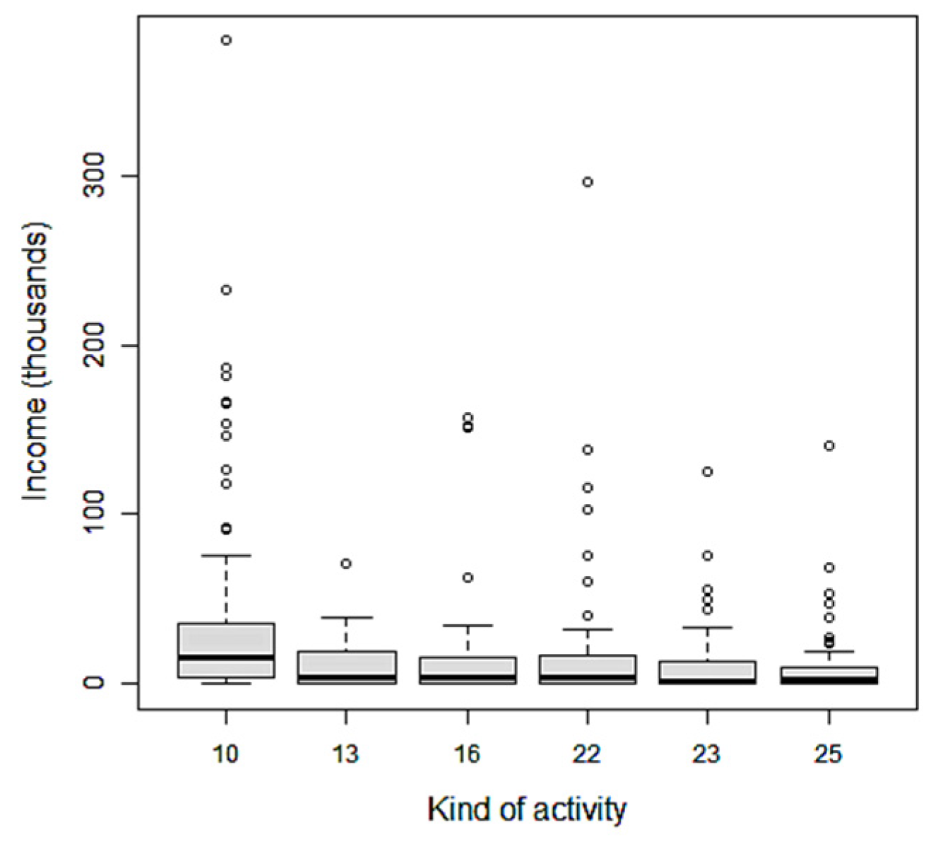
The modified data on enterprises’ expenses from the environment protection survey from the Vilnius Gediminas Technical University Repository [42] are used for a simulation study (Figure 1). Enterprises are involved in several activities, all of which are used in Section 4.2.

4.1. Simulation Study for Change Type (a)

In this study, population consists of 60 enterprises belonging to the 16th economic activity; enterprise income is used as a study variable y. The population is stratified by the number of employees (5–17, 18–100, >100) because enterprise income is highly correlated with the number of employees (see

Table 2. Population correlation coefficients between enterprise income and number of employees by the economic activity.

Economic Activity	10	13	16	22	23	25
Correlation coefficient between income and number of employees	0.65	0.71	0.95	0.56	0.85	0.84

) without seeking any optimization.

A stratified simple random sample of size $n=35$ with the proportional allocation of the sample size is selected. At the time of observation, there are $n^{\prime }=33$ enterprises, because some of them are merged and four non-sampled enterprises are joined (joining of enterprises is simulated inside the stratum with the probability $p=0.15$). For the values of ${y^{\prime }}_k$ when $k\in \omega \backslash {\omega }^{\prime }$ (non-sampled enterprises), the ratio imputation for income with respect to the number of employees is used. The relative measures of accuracy (5) and (6) due to joining of the enterprises are presented in

Table 3. Relative measures of accuracy for the estimators of totals in the case of enterprise joining.

	$\mathit{R}\mathit{d}\mathit{i}\mathit{f}\mathit{f}({{\widehat{\mathit{t}}}^{\prime }}_{\mathit{y}})$	$\mathit{R}\mathit{V}\widehat{\mathit{a}}\mathit{r}({{\widehat{\mathit{t}}}^{\prime }}_{\mathit{y}})$	$\mathit{R}\mathit{d}\mathit{i}\mathit{f}\mathit{f}({\widehat{\mathit{t}}}_{\mathit{y}}^{*})$	$\mathit{R}\mathit{V}\widehat{\mathit{a}}\mathit{r}({\widehat{\mathit{t}}}_{\mathit{y}}^{*})$
$p=0.15$	0.0344	−0.3501	−0.0183	0.5341
$p=0.25$	−0.0425	−0.6092	0.2142	1.0416

. The same measures of accuracy are calculated for the enterprise joining probability $p=0.25$. In this case, $n^{\prime }=29$ and five non-sampled enterprises are joined.

Simulation results show a non-significant relative bias for the estimator of total with recalculated inclusion probabilities ${\widehat{t^{\prime }}}_y$. The relative bias for ${\widehat{t}}_y^{*}$ (the estimator with initial inclusion probabilities and imputed values for study variable of non-sampled but merged enterprises) is increasing with increasing joining probability $p$. Estimates for relative variances $RV\widehat{a}r({{\widehat{t}}^{\prime }}_y)$ and $RV\widehat{a}r({\widehat{t}}_y^{*})$ of both estimators, ${\widehat{t^{\prime }}}_y$ and ${\widehat{t}}_y^{*}$, increase with the increasing joining probability p. Simulation results in Table 3 show that adjustment of the inclusion probabilities due to enterprise joining is worth using.

4.2. Simulation Study for Change Type (c)

A simulated population consists of 2968 enterprises belonging to six economic activities (Figure 1). It is an enterprise data-based population of 379 records duplicated eight times, from which 64 enterprises with the largest number of employees are removed. As it is mentioned in Section 4.1, each activity is stratified by the number of employees into three strata without any optimization. An $n=1196$-size simple random stratified sample with a proportional allocation of a sample size is used for a study. Enterprise income is estimated. Enterprise size changes are simulated with probabilities $p=0.05$, 0.1, 0.15. The totals for each activity are estimated, and relative stratum biases and relative stratum variance changes for the estimator of the total, are presented in

Table 4. Relative biases $RBias\left({\widehat{\widehat{t}}}_{yh}\right)$ for estimators of totals in the strata.

Economic Activity	p = 0.03			p = 0.1			p = 0.18
	Stratum 1	Stratum 2	Stratum 3	Stratum 1	Stratum 2	Stratum 3	Stratum 1	Stratum 2	Stratum 3
10	4.19	4.87	1.28	−0.90	−0.88	−0.54	18.51	9.40	1.04
13	1.78	2.03	1.45	4.12	4.79	1.21	5.34	5.96	1.10
16	6.33	1.46	1.46	6.00	4.51	0.96	11.24	5.48	0.77
22	2.60	1.52	1.49	6.74	3.63	0.99	9.88	3.36	1.00
23	1.53	1.80	1.47	1.64	4.39	1.20	8.56	4.80	1.06
25	2.34	1.55	1.46	3.02	2.20	1.22	4.40	2.46	1.08
Total	2.84	2.40	1.37	4.71	4.60	1.12	8.43	5.39	1.01

and

Table 5. Relative variance changes $RV\widehat{a}r\left({\widehat{\widehat{t}}}_{yh}\right)$ for the estimators of totals in the strata.

	p = 0.03				p = 0.1				p = 0.18
Economic Activity	Stratum 1	Stratum 2	Stratum 3	Change in the Total	Stratum 1	Stratum 2	Stratum 3	Change in the Total	Stratum 1	Stratum 2	Stratum 3	Change in the Total
10	28	69	220	219	301	112	214	214	867	203	186	186
13	49	3	58	56	45	20	56	55	76	29	51	51
16	38	0	58	57	153	20	51	51	575	31	45	44
22	47	1	34	33	198	19	27	27	451	33	23	24
23	−1	0	46	44	0	8	42	40	941	10	37	36
25	1	0	49	43	28	1	53	47	56	2	49	43
Total	18	10	163	161	85	27	158	156	285	46	137	136

. The following expressions are used for relative biases and relative variance changes for the estimator of the total in the strata:

$$RBias\left({\widehat{\widehat{t}}}_{yh}\right)=\frac{{\widehat{\widehat{t}}}_{yh}-t_{yh}}{t_{yh}},RV\widehat{a}r\left({\widehat{\widehat{t}}}_{yh}\right)=\frac{V\widehat{a}r\left({\widehat{\widehat{t}}}_{yh}\right)-V\widehat{a}r\left({\widehat{t}}_{yh}\right)}{V\widehat{a}r\left({\widehat{t}}_{yh}\right)}.$$

Here, $V\widehat{a}r\left({\widehat{t}}_{yh}\right)$ is the Horvitz–Thompson estimator of the variance for the estimator of the total in the case of simple random sampling in the strata, if there are no changes.

The bottom line of Table 4 is attained as a relative bias of the total in the population of Stratum 1, Stratum 2 and Stratum 3 for all economic activities together.

Except for Stratum 3, one can observe that the relative bias is often increasing with an increase in the probability p to move to the neighbouring strata. Populations in each economic activity are very skewed (Figure 1). Stratum 3 of the largest enterprises receives comparatively small newcomers, and they do not cause a big bias in this stratum. The stratum of the smallest enterprises receives middle-sized newcomers, which have a considerable influence on the stratum income, and the bias increases with the increase in the probability p to change the stratum. Stratum 2 of medium-sized enterprises experiences the effects of small and big newcomers with enterprises in both directions, both to the strata of smaller and to the strata of larger enterprises. It is the most mobile stratum, and its relative bias slightly increases with the increase in the probability p to change the stratum. The summary relative biases on the bottom show the same tendency.

Simulation results in Table 5 show relative changes in stratum variances for the estimator of the total when enterprises migrate between strata, and the “change of total” shows the relative change in the variance for the whole estimator of the total in economic activity. All values of the relative changes in the variance for all the estimators of the total are very high, which is due to the very skewed population.

Medium-sized strata have the lowest relative variance, while other strata have higher relative variances which increase with the increasing probability to move from the strata, except for the highest income strata. This highest income strata also influence the relative change in the stratum total variance, which decreases insignificantly with increasing probability $p$.

Enterprises coming to small-size enterprise stratum are only middle-size, but their income are, on average, higher than the income of the receiving stratum. This causes high relative bias for the estimator of total and high relative variance estimates for the estimator of the total, with respect to the estimator of variance when there are no enterprise stratum changes in the receiving stratum.

The large-size enterprise stratum receives only smaller-size enterprises from the neighbouring stratum, and its estimate of total income has a negative relative bias.

The stratum of the medium-size enterprises is the receiver of the small-size enterprises and large-size enterprises; at the same time, it is left by some medium-size enterprises. Despite the appearance of some relative bias of the estimator, their relative estimators for the variance of the estimator of the total is the lowest.

With the increasing probability for enterprise to change the stratum, relative accuracy measures for the small-size enterprise strata and medium-size enterprise strata are increasing, but no effect is observed for large-size enterprises.

Estimates for a total of the whole study population remain almost unbiased. Relative estimates for the variance of the total do not differ significantly with increasing migration probability $p$.

5. Results

A simple random stratified sample is assumed. Three cases of changes in the sampling unit (SU) structure between sample selection and data collection are studied.

(a)

A sampling unit has joined another sampling unit possibly from a different stratum. First and second order inclusion probabilities for the observed sample elements are recalculated. Consequently, a newly adjusted unbiased Horvitz–Thompson estimator of total, its variance and an unbiased estimator for variance are applied. The simulation results show that the relative change of the bias and the relative change of the estimator of variance in the case when there were no changes increases with an increasing probability of changes.

(b)

Sampling units split into the multiple parts and data are received from that part of the split units which are successive of the selected ones. Imputation or an estimator for a two-phase sampling is proposed.

(c)

Another value for the classification variable is reported, i.e., the sampling unit migrated to the neighbouring stratum before data collection. A model for a change of the classification variable is assumed. The new estimator of the total, its variance and variance estimator are obtained. The simulation results show that the relative increase in the bias and the relative increase in variance when there were no changes increase with an increasing probability of migration.

In Case (c), an assumption is made that enterprises change the stratum with equal probabilities and only two neighbouring strata participate in the exchange process with some fixed stratum. This assumption can be relaxed, allowing enterprises to have different probabilities to leave and enter the stratum, and more strata may participate in the exchange.

In order to apply the results in practice, the probability of enterprises changing stratum should be estimated. The probability of enterprises changing the stratum between sample selection and data collection may change over time. Careful study of a specific enterprise population may suggest other models. The relevance of this problem has been demonstrated by real-life surveys.

The methods presented in the article are based on the assumption that there is no non-response and that the joining of units within the sampling frame (Case (a)) or changing of strata (Case (c)) is completely random, i.e., it is not related either to the stratification variable or to the study variable. In reality, several kinds of unit errors may appear at the same time; however, as it was pointed out in the Introduction, only one kind of error at a time is studied in this article.

Changes in the composition of the sampling unit between sample selection and data collection is only one of the problems in enterprise surveys. A much larger number of problems was discussed at the 6th International Conference on the Establishment Surveys [43] and other conferences.

6. Discussion

As we see, the Horvitz–Thompson estimator is inefficient in the case of sampling units changing the stratum. Some smoothing estimator is needed.

Units coming from the neighbouring stratum may significantly change an estimator of the total and its variance in the target stratum because of several reasons: values of the study variable of the coming unit may differ significantly from the values of the units in the target stratum; values of the study variable may be similar in both strata, but the weights may differ significantly; both reasons are possible. If the value of the coming unit differs from the values of the units in the target stratum, it can be dealt with as an outlier. If the weights of the coming units differ significantly from the weights in the target stratum, it is proposed to smooth them by Beaumont [44,45]. Smoothed weights are obtained by applying a suitable model for design weights. One of the methods proposed gives smoothed calibration weights. The author proposes to estimate a mean squared error of the smoothed estimator by bootstrap.

Direct estimators based on sampling design and assumptions on enterprise migration are presented in the article. Due to migration of the sampling units between strata, design weights become unequal, and the population size changes and becomes unknown. No nonresponse is assumed, and no auxiliary variables are used.

Usually, more imperfections appear in the real sample surveys, where some of the sampling units do not report their data, hence the presence of nonresponse. In order to adjust the estimator for frame imperfections and nonresponse, a calibration estimator using auxiliary data is used [46]. In order to reduce the variance of the estimator, auxiliary variables should be well correlated with the study variable.

Nowadays, there are many databases and unstructured data on the internet. It may therefore appear that it should be enough to take a large amount of data from various sources to solve the estimation problem. Unfortunately, some of these data sources are characterised by survey population undercoverage and selection bias; therefore, for integration of such data sources, probability survey data are needed as one of the components giving a jamb. The latter is currently a popular topic among survey statisticians [47,48]. For this reason, further studies into the quality of sample surveys will be necessary.