
Family of Distributions Derived from Whittaker Function


Abstract
:1. Introduction
2. Whittaker Distribution
- 1-
- 2-
- 3-
- is a non-decreasing and right continuous function.
3. Statistical Properties
- The Laplace transformation is.
- The rth moment about the origin is
- The mean is .
- The variance is .
- The mode of for is .
- The measures of skewness , kurtosis , and the coefficient of variation of distribution are, respectively, , , and .
- The survival function is .
- The hazard function is .
- The Laplace transformation: , by using (3).
- The rth moment function is, By using (3).
- We have from II that, and
- The variance is given by
- The mode can be obtained by differentiating the pdf of with respect to as follows, .
- 1-
- .
- 2-
- 3-
- .
- .
- . □
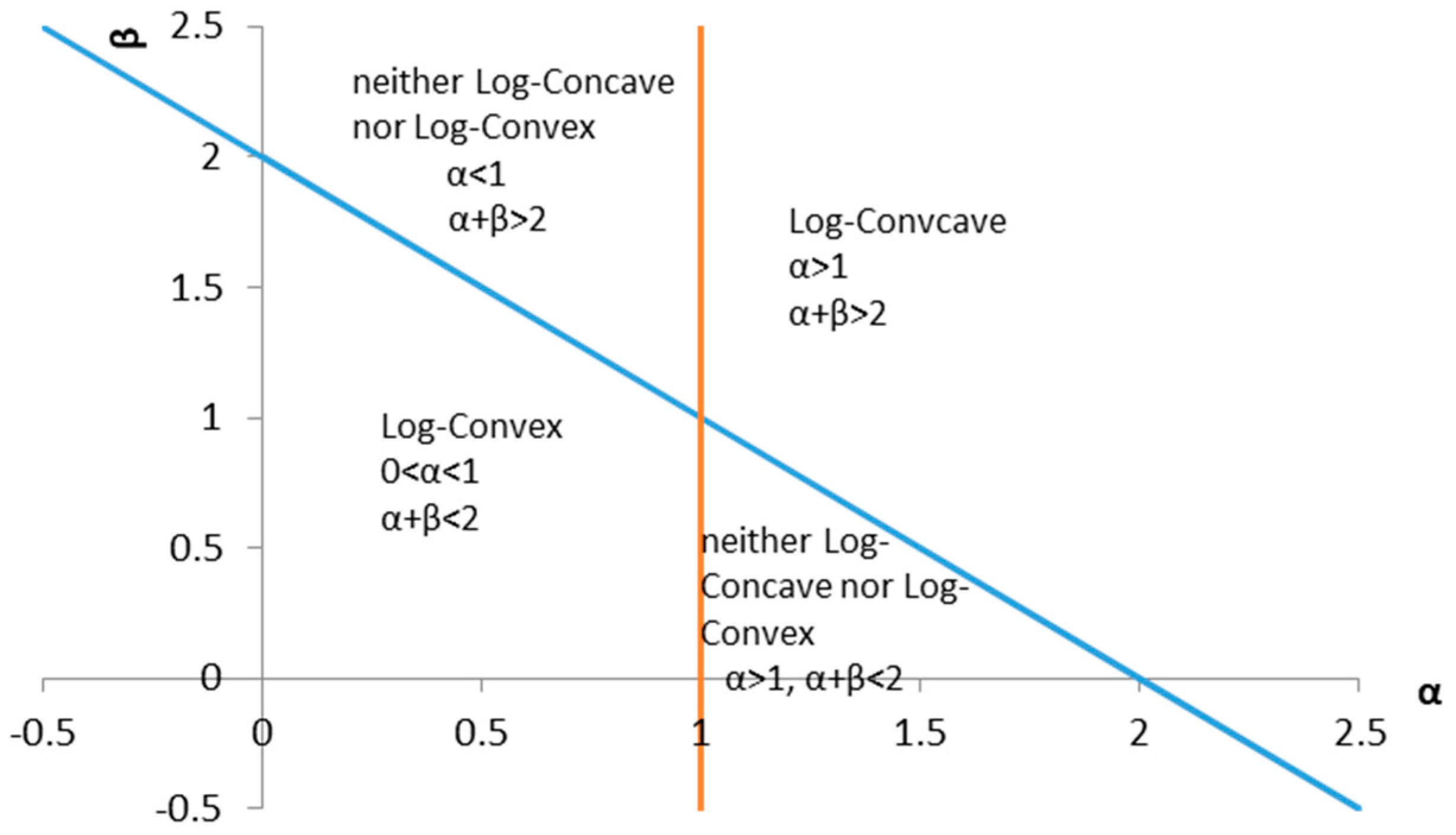
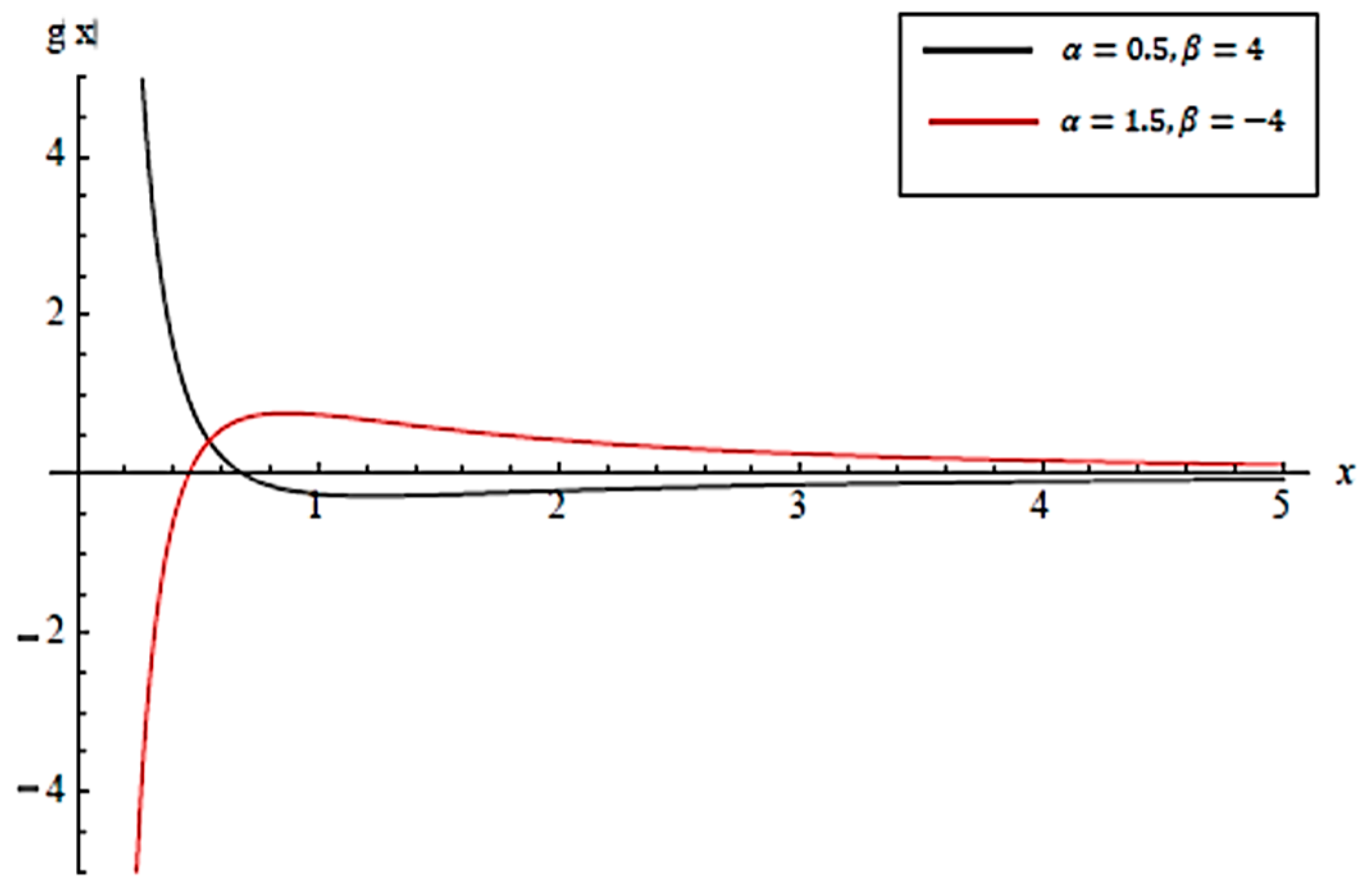
- (a)
- Forandis log-concave.
- (b)
- Forandis log-convex.
- The Whittaker distribution has a monotonic likelihood ratio in x with respect towhen the other parameters are constant.
- The Whittaker distribution has a monotonic likelihood ratio in x with respect towhen the other parameters are constant.
- The Whittaker distribution has a monotonic likelihood ratio in x with respect towhen the other parameters are constant and .
- I
- Let . Then, where .
- II.
- The proof is similar to that of I.
- II.
- For , we acquire where
Percentiles
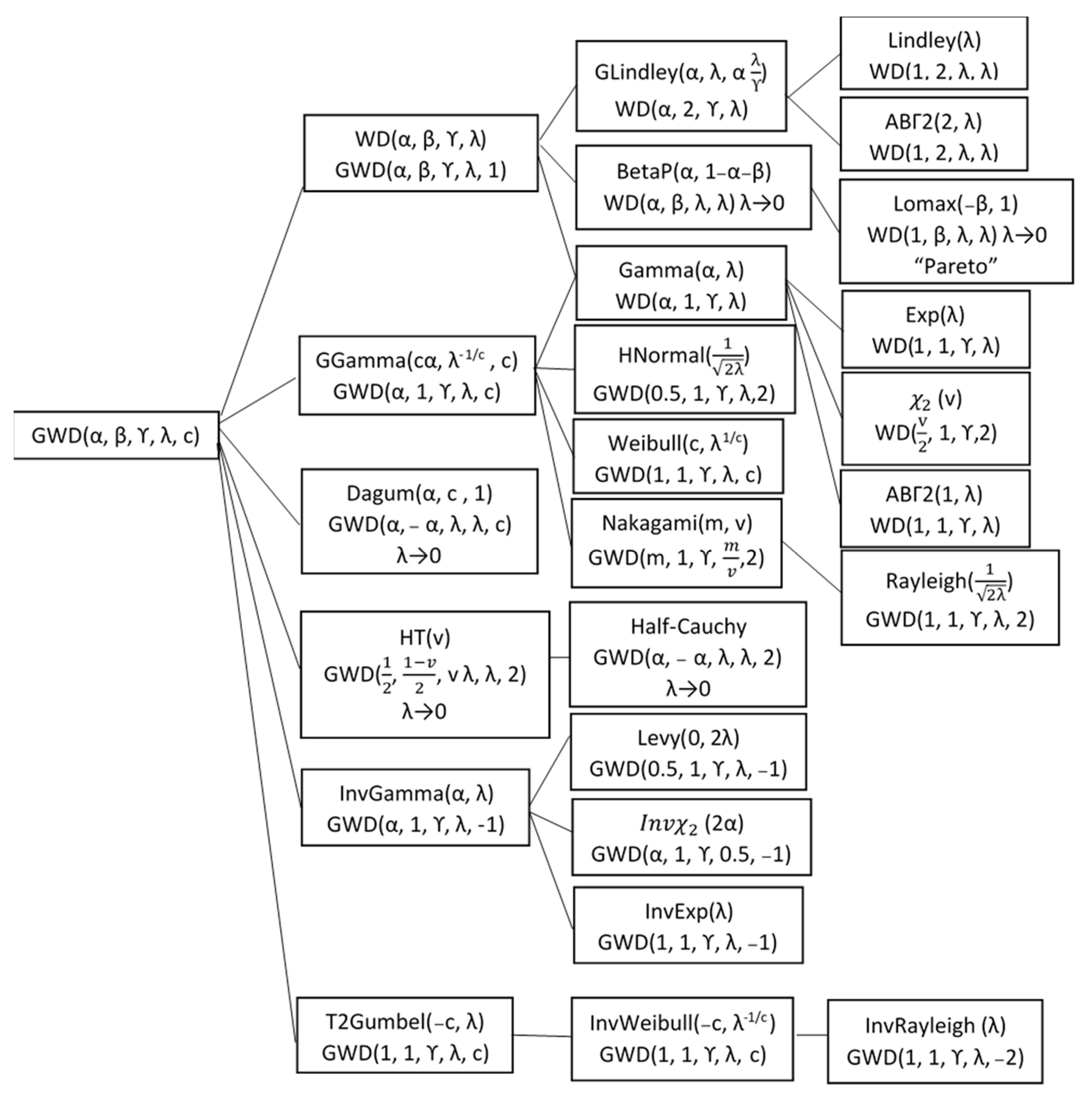
4. Special Cases
4.1. Generalized Lindley Distribution
4.2. Beta Prime Distribution
4.3. Generalized Gamma Distribution
- (a)
- If and , the generalized Whittaker distribution is reduced to the Nakagami distribution [26].
- (b)
- If , and , the generalized Whittaker distribution is reduced to Rayleigh distribution [27].
- (c)
- If , and , the generalized Whittaker distribution is reduced to the half-normal distribution.
- (d)
- If and , the generalized Whittaker distribution is reduced to the Weibull distribution.
- (e)
- If and , the generalized Whittaker distribution is reduced to the gamma distribution.
- (f)
- If and , the Whittaker distribution is reduced to an exponential distribution.
- (g)
- If , and , the Whittaker distribution is reduced to a chi-square distribution with n degrees of freedom.
4.4. Dagum Distribution
4.5. Half-t Distribution
4.6. Inverse Gamma Distribution
- (a)
- If and , the generalized Whittaker distribution is reduced to Lévy distribution [29].
- (b)
- If , and , the generalized Whittaker distribution is reduced to the inverse exponential distribution.
- (c)
- If , , and , the generalized Whittaker distribution is reduced to the inverse chi-square distribution.
4.7. Type-2 Gumbel Distribution
5. Estimation
5.1. Method of Moments
5.2. Maximum Likelihood Estimates
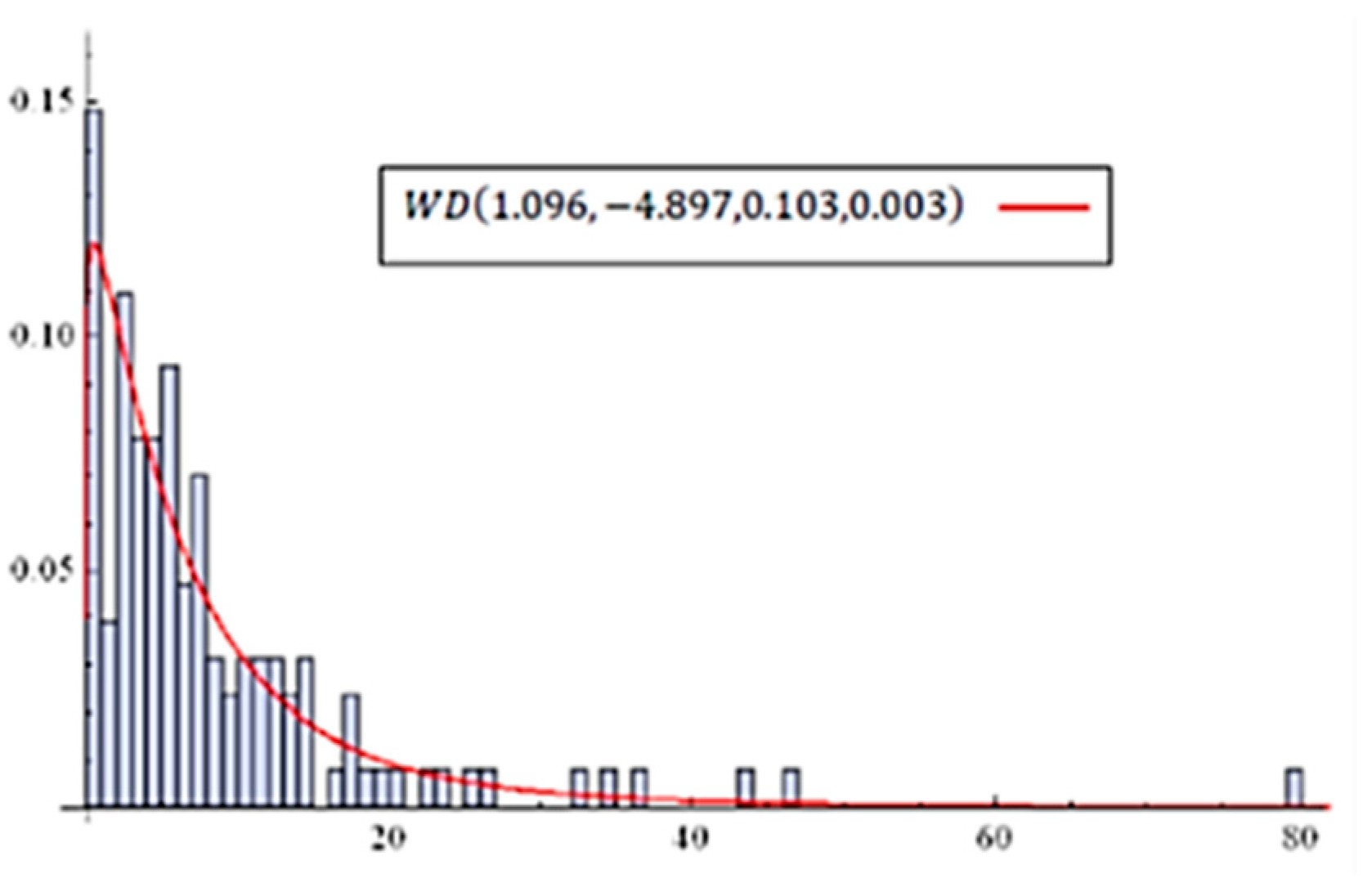
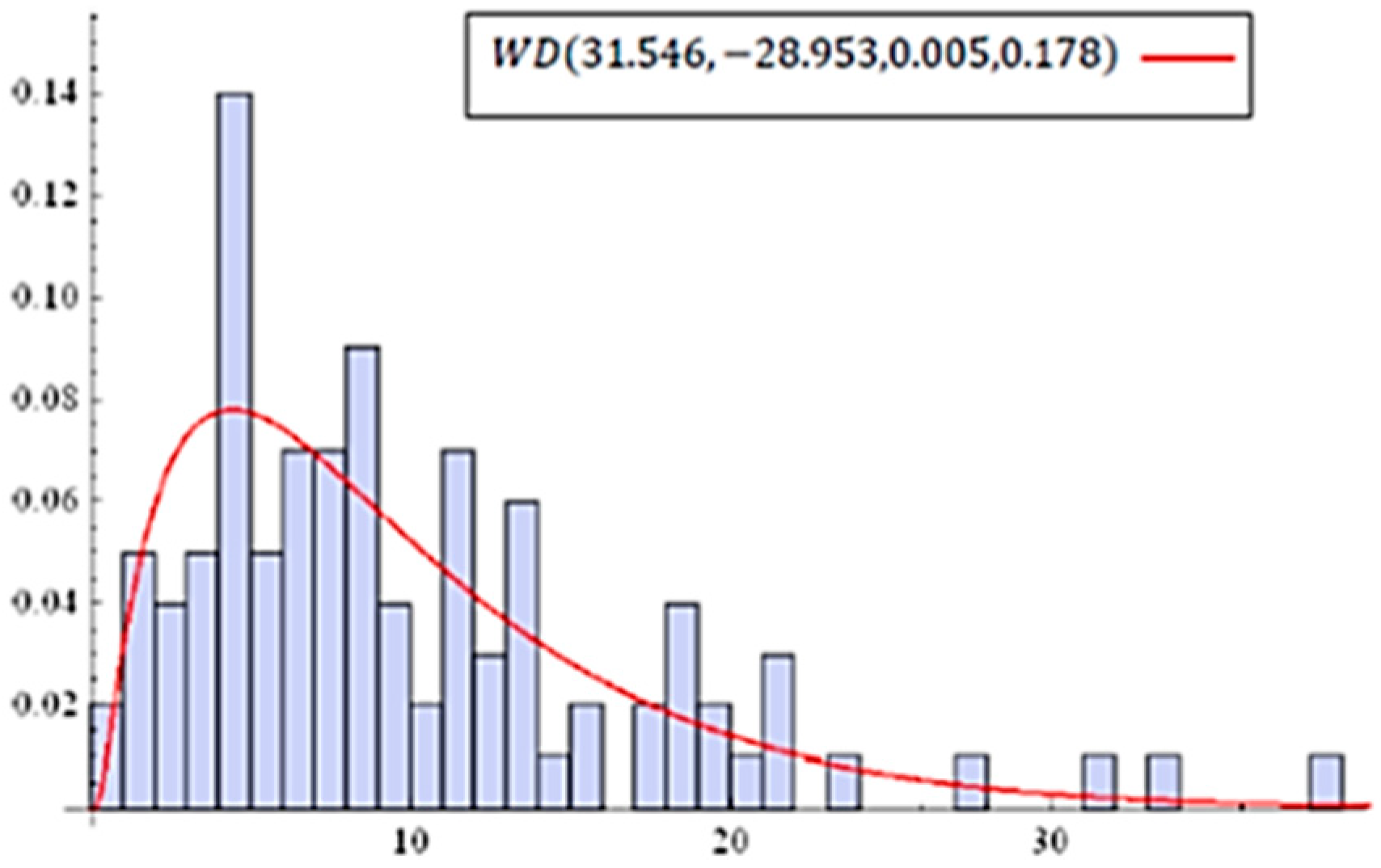
6. Validations
7. Conclusions
Author Contributions
Funding
Institutional Review Board Statement
Informed Consent Statement
Data Availability Statement
Conflicts of Interest
Appendix A
Appendix B
References
- Abramowitz, M.; Stegun, I.A. Handbook of Mathematical Functions with Formulas, Graphs, and Mathematical Tables; 9th Printing; Dover: New York, NY, USA, 1972. [Google Scholar]
- Gradshteyn, I.S.; Ryzhik, I.M. Table of Integrals, Series, and Products, 7th ed.; Elsevier: Burlington, MA, USA, 2007. [Google Scholar]
- Bateman, H. Tables of Integral Transforms [Volumes I & II]; McGraw-Hill Book Company: New York, NY, USA, 1954; Volume 1. [Google Scholar]
- McKay, A.T. A Bessel function distribution. Biometrika 1932, 1, 39–44. [Google Scholar] [CrossRef]
- Laha, R.G. On some properties of the Bessel function distributions. Bull. Calcutta. Math. Soc. 1954, 46, 59–72. [Google Scholar]
- Malik, H.J. Exact distribution of the product of independent generalized gamma variables with the same shape parameter. Ann. Math. Stat. 1968, 39, 1751–1752. [Google Scholar] [CrossRef]
- Pitman, J.; Yor, M.A. decomposition of Bessel bridges. Z. Wahrscheinlichkeit. 1982, 59, 425–457. [Google Scholar] [CrossRef]
- McDonald, J.B. Some generalized functions for the size distribution of income. In Modeling Income Distributions and Lorenz Curves; Springer: New York, NY, USA, 2008; pp. 37–55. [Google Scholar]
- Gordy, M.B. Computationally convenient distributional assumptions for common-value auctions. Comput. Econ. 1998, 12, 61–78. [Google Scholar] [CrossRef]
- Gupta, A.K.; Nagar, D.K. Matrix Variate Distributions; Chapman & Hall/CRC: Washington, DC, USA, 2000. [Google Scholar]
- McNeil, A.J. The Laplace Distribution and generalizations: A revisit with applications to communications, economics, engineering, and finance. J. Am. Stat. Assoc. 2002, 97, 1210–1211. [Google Scholar] [CrossRef]
- Nagar, D.Y.; Zarrazola, E. Distributions of the product and the quotient of independent Kummer-beta variables. Sci. Math. Jpn. 2005, 61, 109–118. [Google Scholar]
- Sánchez, L.E.; Nagar, D.K. Distributions of the product and the quotient of independent beta type 3 variables. Far. East. J. Theor. Stat. 2005, 17, 239. [Google Scholar]
- Küchler, U.; Tappe, S. Bilateral gamma distributions and processes in financial mathematics. Stoch. Process. Appl. 2008, 118, 261–283. [Google Scholar] [CrossRef] [Green Version]
- Zarrazola, E.; Nagar, D.K. Product of independent random variables involving inverted hypergeometric function type I variables. Ing. Cienc. 2009, 5, 93–106. [Google Scholar]
- Nagar, D.K.; Morán-Vásquez, R.A.; Gupta, A.K. Properties and applications of extended hypergeometric functions. Ing. Cienc. 2014, 10, 11–31. [Google Scholar] [CrossRef] [Green Version]
- Gaunt, R.E. Products of normal, beta and gamma random variables: Stein operators and distributional theory. Braz. J. Probab. Stat. 2018, 32, 437–466. [Google Scholar] [CrossRef] [Green Version]
- Shakil, M.; Singh, J.N.; Kibria, B.G. On a family of product distributions based on the Whittaker functions and generalized Pearson differential equation. Pak. J. Statist. 2010, 26, 111–125. [Google Scholar]
- Shakil, M.; Kibria, B.G.; Singh, J.N. A new family of distributions based on the generalized Pearson differential equation with some applications. Austrian J. Stat. 2010, 39, 259–278. [Google Scholar] [CrossRef]
- Zakerzadeh, H.; Dolati, A. Generalized Lindley distribution. J. Math. Ext. 2009, 3, 13–25. [Google Scholar]
- Lindley, D.V. Fiducial distributions and Bayes’ theorem. J. R Stat. Soc. Ser. B Stat. Methodol. 1958, 1, 102–107. [Google Scholar] [CrossRef]
- Johnson, N.L.; Kotz, S.; Balakrishnan, N. Continuous Univariate Distributions, 2nd ed.; Wiley: Hoboken, NJ, USA, 1995; Volume 2, ISBN 0-471-58494-0. [Google Scholar]
- Lomax, K.S. Business failures: Another example of the analysis of failure data. J. Am. Stat. Assoc. 1954, 49, 847–852. [Google Scholar] [CrossRef]
- Arnold, B.C. Pareto Distributions; International Co-operative Publishing House: Fairlan, MD, USA, 1983. [Google Scholar]
- Stacy, E.W. A generalization of the gamma distribution. Ann. Math. Stat. 1962, 33, 1187–1192. [Google Scholar] [CrossRef]
- Nakagami, M. The m-Distribution—A General Formula of Intensity Distribution of Rapid Fading. Stat. Methods Radio Wave Propag. 1960, 1, 3–36. [Google Scholar]
- Beckmann, P. Rayleigh distribution and its generalizations. Radio Sci. J. Res. NBS/USNC-URSIs 1962, 68d, 927–932. [Google Scholar] [CrossRef]
- Dagum, C. A model of income distribution and the conditions of existence of moments of finite order. Bull. Int. Stat. Inst. 1975, 46, 199–205. [Google Scholar]
- Lévy, P. Calcul des probabilités. Rev. Metaphys. Morale 1926, 33, 3–6. [Google Scholar]
- Gumbel, E.J. Statistics of Extremes; Columbia University Press: New York, NY, USA, 1958. [Google Scholar]
- Treyer, V.N. Doklady Acad. Nauk, Belorus, U.S.S.R., 1964.
- Hallin, M.; Ingenbleek, J.F. The swedish automobile portfolio in 1977: A statistical study. Scand. Actuar. J. 1983, 1, 49–64. [Google Scholar] [CrossRef]
- Lee, E.T.; Wang, J.W. Statistical Methods for Survival Data Analysis, 3rd ed.; Wiley: Hoboken, NJ, USA, 2003. [Google Scholar]
- Bjerkedal, T. Acquisition of Resistance in Guinea Pies infected with Different Doses of Virulent Tubercle Bacilli. Am. J. Hyg. 1960, 72, 130–148. [Google Scholar] [PubMed]
- Ghitany, M.E.; Al-Mutairi, D.K.; Nadarajah, S. Zero-truncated Poisson–Lindley distribution and its application. Math. Comput. Simul. 2008, 79, 279–287. [Google Scholar] [CrossRef]


| Data Set 1 | Data Set 2 | Data Set 3 | Data Set 4 | |||||
|---|---|---|---|---|---|---|---|---|
| Model | MLE Parameters | Log(L) | MLE Parameters | Log(L) | MLE Parameters | Log(L) | MLE Parameters | Log(L) |
| −3768.62 | −400.762 | −94.2268 | −316.930 | |||||
| −3768.71 | −400.815 | −94.2291 | −316.931 | |||||
| Log-normal | −3788.58 | −406.802 | −97.5222 | −319.174 | ||||
| Normal | −3773.45 | −482.883 | −104.106 | −339.312 | ||||
| −406.447 | −92.9256 | −317.086 | ||||||
| Generalized Gamma | −3774.44 | −401.66 | −94.2268 | −317.225 | ||||
| Weibull | −3818.69 | 8.2303 = 0.9227 | −402.191 | k = 1.8254 | −95.790 | 10.9553
k = 1.4585 | −318.731 | |
| Gamma | −3773.27 | 0.9155 0.1068 | −402.624 | −94.2291 | −317.3 | |||
| Exponential | −402.96 | |||||||
| Generalized Lindley | −3773.13 | −407.868 | −94.0893 | −317.836 | ||||
| Lindley | −417.924 | |||||||
| Data Set 1 | Data Set 2 | Data Set 3 | Data Set 4 | |||||
|---|---|---|---|---|---|---|---|---|
| WD vs | Test statistic | p-value | Test statistic | p-value | Test statistic | p-value | Test statistic | p-value |
| Log-normal | 2.8733 | 0.0041 | 1.4188 | 0.1559 | 0.3568 | 0.7212 | 0.1284 | 0.8979 |
| Normal | 0.8716 | 0.3834 | 4.4671 | <0.001 | 2.0183 | 0.0436 | 3.5893 | 0.0003 |
| Johnson | (Johnson SL) 2.3096 | 0.0209 | (Johnson SU) −1.0613 | 0.2885 | (Johnson SB) 0.3735 | 0.7088 | ||
Publisher’s Note: MDPI stays neutral with regard to jurisdictional claims in published maps and institutional affiliations. |
© 2022 by the authors. Licensee MDPI, Basel, Switzerland. This article is an open access article distributed under the terms and conditions of the Creative Commons Attribution (CC BY) license (https://creativecommons.org/licenses/by/4.0/).
Share and Cite
Omair, M.A.; Tashkandy, Y.A.; Askar, S.; Alzaid, A.A. Family of Distributions Derived from Whittaker Function. Mathematics 2022, 10, 1058. https://doi.org/10.3390/math10071058
Omair MA, Tashkandy YA, Askar S, Alzaid AA. Family of Distributions Derived from Whittaker Function. Mathematics. 2022; 10(7):1058. https://doi.org/10.3390/math10071058
Chicago/Turabian StyleOmair, Maha A., Yusra A. Tashkandy, Sameh Askar, and Abdulhamid A. Alzaid. 2022. "Family of Distributions Derived from Whittaker Function" Mathematics 10, no. 7: 1058. https://doi.org/10.3390/math10071058
APA StyleOmair, M. A., Tashkandy, Y. A., Askar, S., & Alzaid, A. A. (2022). Family of Distributions Derived from Whittaker Function. Mathematics, 10(7), 1058. https://doi.org/10.3390/math10071058