Abstract
In this paper, a generalized nonlinear Schrödinger (gNLS) equation with time-varying coefficients is analytically studied using its Lax representation and the associated Riemann-Hilbert (RH) problem equipped with a symmetric scattering matrix in the Hermitian sense. First, Lax representation and the associated RH problem of the considered gNLS equation are established so that solution of the gNLS equation can be transformed into the associated RH problem. Secondly, using the solvability of unique solution of the established RH problem, time evolution laws of the scattering data reconstructing potential of the gNLS equation are determined. Finally, based on the determined time evolution laws of scattering data, the long-time asymptotic solution and N-soliton solution of the gNLS equation are obtained. In addition, some local spatial structures of the obtained one-soliton solution and two-soliton solution are shown in the figures. This paper shows that the RH method can be extended to nonlinear evolution models with variable coefficients, and the curve propagation of the obtained N-soliton solution in inhomogeneous media is controlled by the selection of variable–coefficient functions contained in the models.
Keywords:
gNLS equation with time-varying coefficients; Lax representation; RH problem; scattering data; long-time asymptotic solution; N-soliton solution MSC:
37K40; 37K10; 35Q15; 35C08
1. Introduction
Nonlinear problems are full of challenges, and these have attracted the extensive attention of researchers. One of the important achievements of nonlinear mathematical physics in recent decades is the discovery of certain nonlinear partial differential equations (PDEs) with important applications and analytical solutions. For example, the classical NLS equation has practical applications in many fields [1], including optics, oceanography, biology, economics and so on. There are many effective methods for solving nonlinear PDEs analytically, such as inverse scattering method [2], Darboux transformation [3], Hirota bilinear method [4] and other methods [5,6,7,8,9,10,11,12,13,14].
When an inhomogeneous medium is considered, the variable–coefficient model is usually closer to the essence of the phenomenon. Generally, solving variable–coefficient equations is more difficult than solving constant-coefficient ones. In most cases, it is necessary to embed appropriate coefficient functions in the solution process of the existing analytical methods, see [15] for an ingenious work extending inverse scattering method to deal with a variable–coefficient NLS equation. Owing to the fact that Schrödinger-type equations are widely used in many fields and differential equations with variable–coefficient functions often model dynamic processes in non-uniform media, this paper considers a model in nonlinear fiber optics, namely the following gNLS equation with gain [16]:
where ; the three functions , and of propagation distance represent the group velocity dispersion parameter, nonlinearity parameter and distributed gain function, respectively; denotes the module of ; and is the imaginary unit. For convenience, we take the transformations:
Then, Equation (1) is converted to the gNLS equation with time-varying coefficients:
Here, and are assumed to be real integrable functions, while and all its partial derivatives with respect to and approach zero quickly enough as .
The analytical method adopted in this paper for Equation (3) is the RH method [17], which was developed based on the IST [2]. The RH method is an analytical method that does not need to solve the Gel’fand-Levitan-Marchenko integral equation and can also analyze the long-time asymptotic behavior of the obtained implicit analytical solutions. In recent years, the RH method has achieved many applications, such as [17,18,19,20,21,22,23,24,25,26,27,28]. One of the important developments of RH method is Deift-Zhou’s nonlinear steepest descent method [18].
The basic idea of the RH method is to establish the relationship between the solution of nonlinear PDE to be solved and the solution of associated solvable RH problem using the eigenfunction, then to solve the RH problem, and finally obtain the solution of nonlinear PDE. In the literature, there are some results, such as [8,16,29,30,31,32,33,34,35], that have been obtained for the gNLS Equation (3). However, as far as we know, there is still no research on the RH problem of Equation (3), and the relevant work is worth exploring. Equation (3) is integrable; the Lax presentation, which provides a basis of the study of the associated RH problem is given in Section 2.
With the help of the given Lax presentation, the associated RH problem is established in Section 3 to connect the solution of Equation (3) and that of the established RH problem, and then the time evolution laws of scattering data in the RH problem are determined. In Section 4, the long-time asymptotic solution and N-soliton solution of Equation (3) are obtained. At the same time, some spatial structures of the obtained one-soliton solution and two-soliton solution are shown by selecting several special cases of the time-varying functions.
2. Lax Presentation and RH Problem
We introduce, in this section, the linear spectral problem in the matrix forms:
where is the complex spectral parameter; is the eigenfunction in matrix form; the notations , and stand for
and the symbol * is complex conjugate.
It is easy to check that the compatibility condition is equivalent to Equation (3). Therefore, we say that the gNLS Equation (3) has Lax integrability, and its Lax representations are Equations (4) and (5).
Considering the asymptotic condition of the previously assumed boundary value that and all its partial derivatives, with respect to and , approach zeros quickly as , we have the asymptotic Jost solution of Equations (4) and (5):
with
By the transformation:
we transform Equations (4) and (5) into the following forms:
so that the eigenfunction has the boundary condition:
where means the boundary conditions of at the positive infinity and negative infinity respectively, and denotes the second-order identity matrix. In the case where the boundary conditions (12) hold, the x-part of the Lax representation, that is, Equation (10) has the solutions [17]:
which enable the following relationships to be established:
by means of the scattering matrix:
Since the determinant [17], which shows that the matrix is reversible, we can see from Equation (15) that and then obtain the inverse matrix of the scattering matrix :
Due to , with standing for the Hermitian conjugate, one knows that the symmetric relation leads to the equalities and .
With the help of notations and , we introduce the matrices:
where and denote the vector in the s-th row and that in the s-th column of , respectively, and and are two special diagonal matrices. Clearly, and enable Equation (10) and its adjoint equation to be true, that is to say:
The Taylor series of gives:
We insert and into Equations (20) and (21) and compare the coefficients of , and then one has
Thus, solution of the gNLS Equation (3) is converted to by the following formula:
with representing the element locations at the intersection of the first row and the second column of . Here, will be determined by the matrix RH problem established by Equations (18) and (19):
where and are the upper and lower half complex planes, respectively; is the set of real numbers; and is the jump matrix:
3. Solvability of RH Problem and Time Evolution Laws for Scattering Data
The RH Problem (25) established above is solvable and always has a unique solution. More detailed proof can be found in [17]; the difference is because the time evolution laws of the scattering data involved are different. In fact, from Equations (15), (18) and (19), we can see that
where the symmetry relation has been used.
When , the RH problem (30) is regular. Then, Plemelj formula [36] can be used to obtain a unique solution of Equation (25):
with
In the case of , the relation makes the numbers of the conjugate zeros of and must be equal. Thus, we suppose that has conjugate zeros and denote the conjugate zeros of as . For the irregular case of the RH Problem (25), we consider the systems of linear equations:
where non-zero row vector and non-zero column vector are solutions of Equations (30) and (31), respectively. The Hermitian conjugate of Equation (30), together with the symmetry relation , gives
Then, Equations (31) and (32) lead to the symmetry relation . Based on these preparations and theorem [37], the irregular RH Problem (25) with can be transformed into a regular one. Thus, we indirectly arrive at the proof that the irregular RH Problem (25) has a unique solution, and therefore the solution of Equation (24) can be determined as follows:
with
The solvability of RH Problem (25) lays a theoretical foundation for the determination of the corresponding scattering data.
Theorem 1.
Letsolve the gNLS Equation (3). Then, the scattering data:
determined by the regular RH problem (30) have the time evolution laws:
Proof of Theorem 1.
It is necessary to rewrite Equation (15) as:
Differentiating the left side of Equation (48) with respect to , we arrive at
by employing Equation (15). It is easy to see from Equation (44) that the left side of Equation (43) solves Equation (11). We, therefore, know that the right side of Equation (43) is a solution of Equation (11). Then, the substitution of the right side of Equation (43) into Equation (11) together with the boundary condition (12) yields
Similarly, we easily see that is also a solution of Equation (11). Putting into Equation (11) and using the boundary condition (12) yields:
Considering Equations (16) and (17) and comparing the elements of Equations (45) and (46), we gain
Solving Equations (47) and (48), we reach Equations (38) and (39). Equation (27) indicates that, if and are the zeros of and , they are also the zeros of and . In view of Equation (49), one can see that and are independent from . This means that Equation (40) is true.
To prove Equations (41) and (42), it is necessary to differentiate Equation (30) with respect to and , and then one has
Using Equations (11) and (18) yields
Substituting Equations (20) and (52) into Equations (50) and (51), we gain
by the usage of Equation (30). Solving Equations (53) and (54), one can obtain Equation (41). In a similar way, Equation (42) can be obtained using Equations (11), (21) and (31). □
4. Long-Time Asymptotic Solution and N-Soliton Solution
Based on Equations (38) and (39), the time evolution laws of the Jump matrix can be determined as follows:
where is determined by Equation (8). Generally, with the above scattering data in Equations (38)–(42), one can obtain solution of the gNLS Equation (3) theoretically. However, we still have difficulty in calculating the integral in Equation (33) for . In this case, the asymptotic solution of the gNLS Equation (3) when can be derived from Equation (24). For instance, if we let and for any , the integral contained in Equation (38) tends to zero at a rate of . We, therefore, obtain the following long-time asymptotic solution of the gNLS Equation (3):
where and are calculated using Equations (36) and (41), while the calculation of can restore to Equation (42) or the symmetry relation .
In the reflectionless case, we next construct an N-soliton solution of the NLS Equation (3). Setting and , and then one has . In this case, Equation (33) is simplified as
To determine in Equation (57), we further select the complex number and let . Then, Equations (41) and (42) give
where
Finally, with the help of Equations (24) and (58)–(60), one obtains the N-soliton solution of NLS Equation (3):
where and can be determined by Equation (60),
As a special case of Equation (61), is selected, and then one has:
Further letting and yields and . Thus, Equation (63) becomes
which can be rewritten as:
Finally, the one-soliton solution of the gNLS Equation (3) can be obtained as follows:
where
In Figure 1, Figure 2, Figure 3 and Figure 4, four spatial structures of the one-soliton solution (66) are shown by selecting the same parameters , , and , however, with different time-varying coefficients: and in Figure 1; and in Figure 2; and in Figure 3; and and in Figure 4. Figure 1, Figure 2, Figure 3 and Figure 4 show that the four bell one-solitons propagating along the negative x-axis have different velocities: variable velocities in Figure 1, Figure 2 and Figure 3 and uniform velocity in Figure 4. Form Equation (67), we can see that and determine the frequency of the soliton vibration.
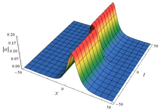
Figure 1.
Spatial structure of the one-soliton solution (66) with and .
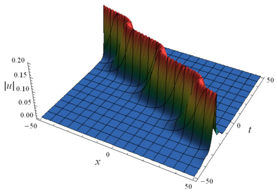
Figure 2.
Spatial structure of the one-soliton solution (66) with and .
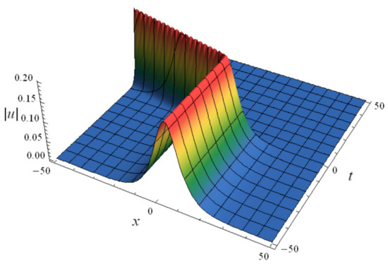
Figure 3.
Spatial structure of the one-soliton solution (66) with and .
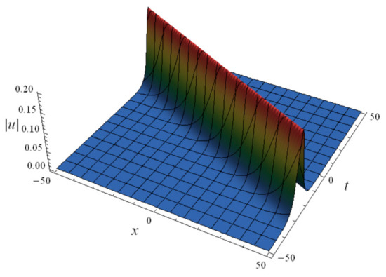
Figure 4.
Spatial structure of the one-soliton solution (66) with and .
When , solution (61) cannot be written as a hyperbolic function like Equation (66). For the selection of , Equation (61) gives
with
where and are determined by Equation (65), and . In Figure 5, Figure 6 and Figure 7, a collision between bell two-solitons determined by solution (68) is shown by setting the parameters , , , , and . It can be seen from Figure 5, Figure 6 and Figure 7 that, after interaction, two solitons moving in the opposite directions along the x-axis move away from each other in the original opposite direction. This is different from the interaction between two solitons with the variable coefficient and the constant coefficient , which continue to move forward after passing through each other as shown in Figure 8, Figure 9 and Figure 10.
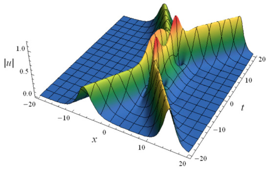
Figure 5.
Spatial structure of the two-soliton solution (68) with and .
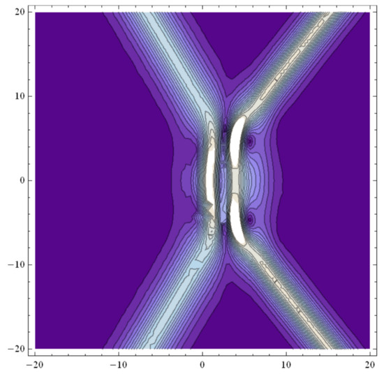
Figure 6.
Contour of the two-soliton solution (68) with and .
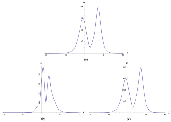
Figure 7.
Interaction of the two-soliton solution (68) with and : (a) , (b) and (c) .
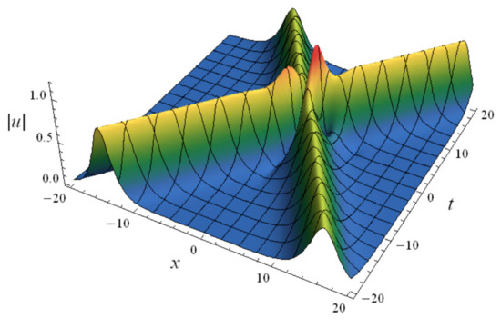
Figure 8.
Spatial structure of the two-soliton solution (68) with and .
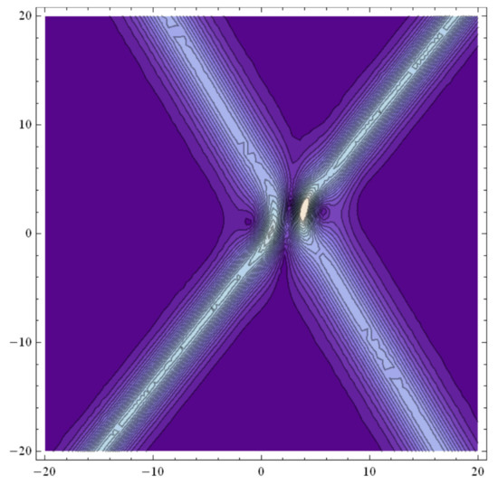
Figure 9.
Contour of the two-soliton solution (68) with and .
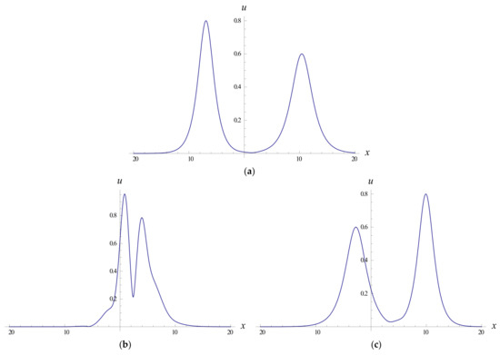
Figure 10.
Interaction of the two-soliton solution (68) with and : (a) , (b) and (c) .
5. Conclusions
Taking the gNLS Equation (3) as an example, this paper presented a positive answer to the feasibility of extending the RH method [17] to nonlinear evolution equations with variable coefficients. Due to the derived Lax representation in Equations (4) and (5) and their transformation forms (10) and (11) with unit boundary values at infinity of spatial independent variables, the solution of the gNLS Equation (3) is transformed into the associated RH problem (30) via Equation (29).
Based on the solvability of the RH Problem (25), we determined the time evolution laws (38)–(42) of the corresponding scattering data, recovered the potential function using the RH method [17] and, finally, obtained the solution (56) with the long-time asymptotic behavior and the N-soliton solution (61). It can be seen from Figure 1, Figure 2, Figure 3 and Figure 4 that four bell one-solitons propagating from the positive x-axis to the negative x-axis possess different velocities, which make their peaks form different motion trajectories, including the kink trajectory in Figure 1, periodic kink trajectory in Figure 2, straight turning trajectory in Figure 3 and straight-line trajectory in Figure 4. This is due to the different selections of the time-varying coefficient function .
Whether the propagation trajectory of the bell soliton peak determined by the one-soliton solution (66) shows a straight line or curve depends on the time-varying coefficient . For the multiple soliton solution (61) with , there will be similar peak curve trajectory characteristics. In fact, for the one-soliton solution (66), this point can be verified mathematically. Specifically, from Equation (66), we determined the modulus of the one-soliton solution (66):
which is a bell soliton solution. The peak coordinates of the bell soliton determined by Equation (71) satisfy the equation:
Clearly, the parameter controlling the peak trajectory of the above bell one-soliton is the propagation velocity . Therefore, selecting as a constant is the reason why the peak trajectory of the bell one-soliton in Figure 4 is a straight line. In addition, it should be pointed out that, when and , the gNLS Equation (3) becomes the classical NLS equation, and the results obtained in this paper can degenerate into the known ones [17]. Recently, some novel solutions [33,34,35] of NLS-type equations with variable coefficients have been obtained. A comparison shows that both the long-time asymptotic solution (63) and the N-soliton solution (61) are different from those in [8,16,29,30,31,32,33,34,35].
Author Contributions
Methodology, B.X.; software, B.X.; writing—original draft preparation, B.X.; writing—review and editing, S.Z. All authors have read and agreed to the published version of the manuscript.
Funding
This research was supported by the Liaoning BaiQianWan Talents Program of China (2019), the Natural Science Foundation of Education Department of Liaoning Province of China (LJ2020002) and the Natural Science Foundation of Xinjiang Autonomous Region of China (2020D01B01).
Institutional Review Board Statement
Not applicable.
Informed Consent Statement
Not applicable.
Data Availability Statement
The data in the manuscript are available from the corresponding author upon request.
Acknowledgments
The authors would like to express their thanks to the anonymous referees for their valuable comments.
Conflicts of Interest
The authors declare no conflict of interest.
References
- Liu, W.M.; Kengne, E. Schrödinger Equations in Nonlinear Systems; Springer Nature Singapore Pte Ltd.: Singapore, 2019. [Google Scholar]
- Gardner, C.S.; Greene, J.M.; Kruskal, M.D.; Miura, R.M. Method for solving the Korteweg-de Vries equation. Phys. Rev. Lett. 1967, 19, 1095–1197. [Google Scholar] [CrossRef]
- Matveev, V.B.; Salle, M.A. Darboux Transformation and Soliton; Springer: Berlin, Germany, 1991. [Google Scholar]
- Hirota, R. Exact envelope-soliton solutions of a nonlinear wave equation. J. Math. Phys. 1973, 14, 805–809. [Google Scholar] [CrossRef]
- Wang, M.L. Exact solutions for a compound KdV-Burgers equation. Phys. Lett. A 1996, 213, 279–287. [Google Scholar] [CrossRef]
- Fan, E.G. Travelling wave solutions in terms of special functions for nonlinear coupled evolution systems. Phys. Lett. A 2002, 300, 243–249. [Google Scholar] [CrossRef]
- He, J.H.; Wu, X.H. Exp-function method for nonlinear wave equations. Chaos Soliton. Fract. 2006, 30, 700–708. [Google Scholar] [CrossRef]
- Zhang, S.; Xia, T.C. A generalized auxiliary equation method and its application to (2 + 1)-dimensional asymmetric Nizhnik-Novikov-Vesselov equations. Phys. A Math. Theor. 2007, 40, 227–248. [Google Scholar] [CrossRef]
- Ma, W.X.; Lee, J.H. A transformed rational function method and exact solutions to 3 + 1 dimensional Jimbo-Miwa equation. Chaos Soliton. Fract. 2009, 42, 1356–1363. [Google Scholar] [CrossRef] [Green Version]
- Tian, S.F. Initial-boundary value problems for the general coupled nonlinear Schrödinger equation on the interval via the Fokas method. J. Diff. Equ. 2016, 262, 506–588. [Google Scholar] [CrossRef]
- Xu, B.; Zhang, S. A novel approach to time-dependent-coefficient WBK system: Doubly periodic waves and singular nonlinear dynamics. Complexity 2018, 2018, 3158126. [Google Scholar] [CrossRef] [Green Version]
- Xu, B.; Zhang, S. Exact solutions with arbitrary functions of the (4 + 1)-dimensional Fokas equation. Therm. Sci. 2019, 23, 2403–2411. [Google Scholar] [CrossRef]
- Xu, B.; Zhang, S. Exact solutions of nonlinear equations in mathematical physics via negative power expansion method. J. Math. Phys. Anal. Geo. 2021, 17, 369–387. [Google Scholar] [CrossRef]
- Zhang, S.; Xu, B. Painlevé test and exact solutions for (1 + 1)-dimensional generalized Broer-Kaup equations. Mathematics 2022, 10, 486. [Google Scholar] [CrossRef]
- Serkin, V.N.; Hasegawa, A.; Belyaeva, T.L. Nonautonomous solitons in external potentials. Phys. Rev. Lett. 2007, 98, 074102. [Google Scholar] [CrossRef]
- Kruglov, V.I.; Peacock, A.C.; Harvey, J.D. Exact self-similar solutions of the generalized nonlinear Schrödinger equation with distributed coefficients. Phys. Rev. Lett. 2003, 90, 113902. [Google Scholar] [CrossRef]
- Yang, J.K. Nonlinear Waves in Integrable and Nonintegrable Systems; SIAM: Philadelphia, PA, USA, 2010. [Google Scholar]
- Deift, P.; Zhou, X. A steepest descent method for oscillatory Riemann-Hilbert problems. Ann. Math. 1993, 137, 295–368. [Google Scholar] [CrossRef] [Green Version]
- Xu, J.; Fan, E.G.; Chen, Y. Long-time asymptotic for the derivative nonlinear Schrödinger equation with step-like initial value. Math. Phys. Anal. Geom. 2013, 16, 253–288. [Google Scholar] [CrossRef] [Green Version]
- Ma, W.X. Riemann-Hilbert problems and N-soliton solutions for a coupled mKdV system. J. Geom. Phys. 2018, 132, 45–54. [Google Scholar] [CrossRef]
- Hu, B.B.; Xia, T.C.; Ma, W.X. Riemann-Hilbert approach for an initial-boundary value problem of the two-component modified Korteweg-de Vries equation on the half-line. Appl. Math. Comput. 2018, 332, 148–159. [Google Scholar] [CrossRef]
- Wang, D.S.; Guo, B.; Wang, X.L. Long-time asymptotics of the focusing Kundu-Eckhaus equation with nonzero boundary conditions. J. Differ. Equ. 2019, 266, 5209–5253. [Google Scholar] [CrossRef]
- Chen, S.Y.; Yan, Z.Y.; Guo, B.L. Long-time asymptotics for the focusing Hirota equation with non-zero boundary conditions at infinity via the Deift-Zhou approach. Math. Phys. Anal. Geom. 2021, 24, 17. [Google Scholar] [CrossRef]
- Guo, H.D.; Xia, T.C. Multi-soliton solutions for a higher-order coupled nonlinear Schrödinger system in an optical fiber via Riemann-Hilbert approach. Nonlinear Dyn. 2021, 103, 1805–1816. [Google Scholar] [CrossRef]
- Li, Z.Q.; Tian, S.F.; Zhang, T.T.; Yang, J.J. Riemann-Hilbert approach and multi-soliton solutions of a variable-coefficient fifth-order nonlinear Schrödinger equation with N distinct arbitrary-order poles. Mod. Phys. Lett. B 2021, 35, 2150194. [Google Scholar] [CrossRef]
- Zhang, B.; Fan, E.G. Riemann-Hilbert approach for a Schrödinger-type equation with nonzero boundary conditions. Mod. Phys. Lett. B 2021, 35, 2150208. [Google Scholar] [CrossRef]
- Wei, H.Y.; Fan, E.G.; Guo, H.D. Riemann-Hilbert approach and nonlinear dynamics of the coupled higher-order nonlinear Schrödinger equation in the birefringent or two-mode fiber. Nonlinear Dyn. 2021, 104, 649–660. [Google Scholar] [CrossRef]
- Xu, B.; Zhang, S. Riemann-Hilbert approach for constructing analytical solutions and conservation laws of a local time-fractional nonlinear Schrödinger equation. Symmetry 2021, 13, 13091593. [Google Scholar] [CrossRef]
- Serkin, V.N.; Hasegawa, A. Novel soliton solutions of the nonlinear Schrödinger equation model. Phys. Rev. Lett. 2000, 85, 4502–4505. [Google Scholar] [CrossRef]
- Kruglov, V.I.; Harvey, J.D. Asymptotically exact parabolic solutions of the generalized nonlinear Schrödinger equation with varying parameters. J. Opt. Soc. Am. B 2006, 23, 2541–2550. [Google Scholar] [CrossRef]
- Serkin, V.N.; Belyaeva, T.L. Optimal control of dark solitons. Optik 2018, 168, 827–838. [Google Scholar] [CrossRef]
- Zhang, S.; Zhang, L.J.; Xu, B. Rational waves and complex dynamics: Analytical insights into a generalized nonlinear Schrödinger equation with distributed coefficients. Complexity 2019, 2019, 3206503. [Google Scholar] [CrossRef]
- Plemelj, J. Riemannsche Funktionenscharen mit gegebener Monodromiegruppe. Monatsch. Math. Phys. 1908, 19, 211–246. [Google Scholar] [CrossRef] [Green Version]
- Zakharov, V.E.; Shabat, A.B. Integration of nonlinear equations of mathematical physics by the method of inverse scattering. II. Funct. Anal. Appl. 1979, 13, 166–174. [Google Scholar] [CrossRef]
- Mai, X.L.; Li, W.; Dong, S.H. Exact solution to the nonlinear Schrödinger equation with time-dependent coefficients. Adv. High Energy Phys. 2021, 2021, 6694980. [Google Scholar] [CrossRef]
- Guo, Q.; Liu, J. New exact solution to the nonlinear Schrödinger equation with variable coefficients. Results Phys. 2020, 16, 102857. [Google Scholar] [CrossRef]
- Kosti, A.A.; Colreavy-Donnelly, S.; Caraffini, F.; Anastassi, Z.A. Efficient computation of the nonlinear Schrödinger equation with time-dependent coefficients. Mathematics 2020, 8, 374. [Google Scholar] [CrossRef] [Green Version]
Publisher’s Note: MDPI stays neutral with regard to jurisdictional claims in published maps and institutional affiliations. |
© 2022 by the authors. Licensee MDPI, Basel, Switzerland. This article is an open access article distributed under the terms and conditions of the Creative Commons Attribution (CC BY) license (https://creativecommons.org/licenses/by/4.0/).