
Quantitative Mean Square Exponential Stability and Stabilization of Linear Itô Stochastic Markovian Jump Systems Driven by Both Brownian and Poisson Noises


Abstract
:1. Introduction
2. Preliminaries
3. Quantitative Mean Square Exponential Stability
4. Quantitative Mean Square Exponential Stabilization
4.1. Stabilization via SFC
4.2. Stabilization via OBC
5. Numerical Algorithm
| Algorithm 1 2-mode case |
|
6. Numerical Examples
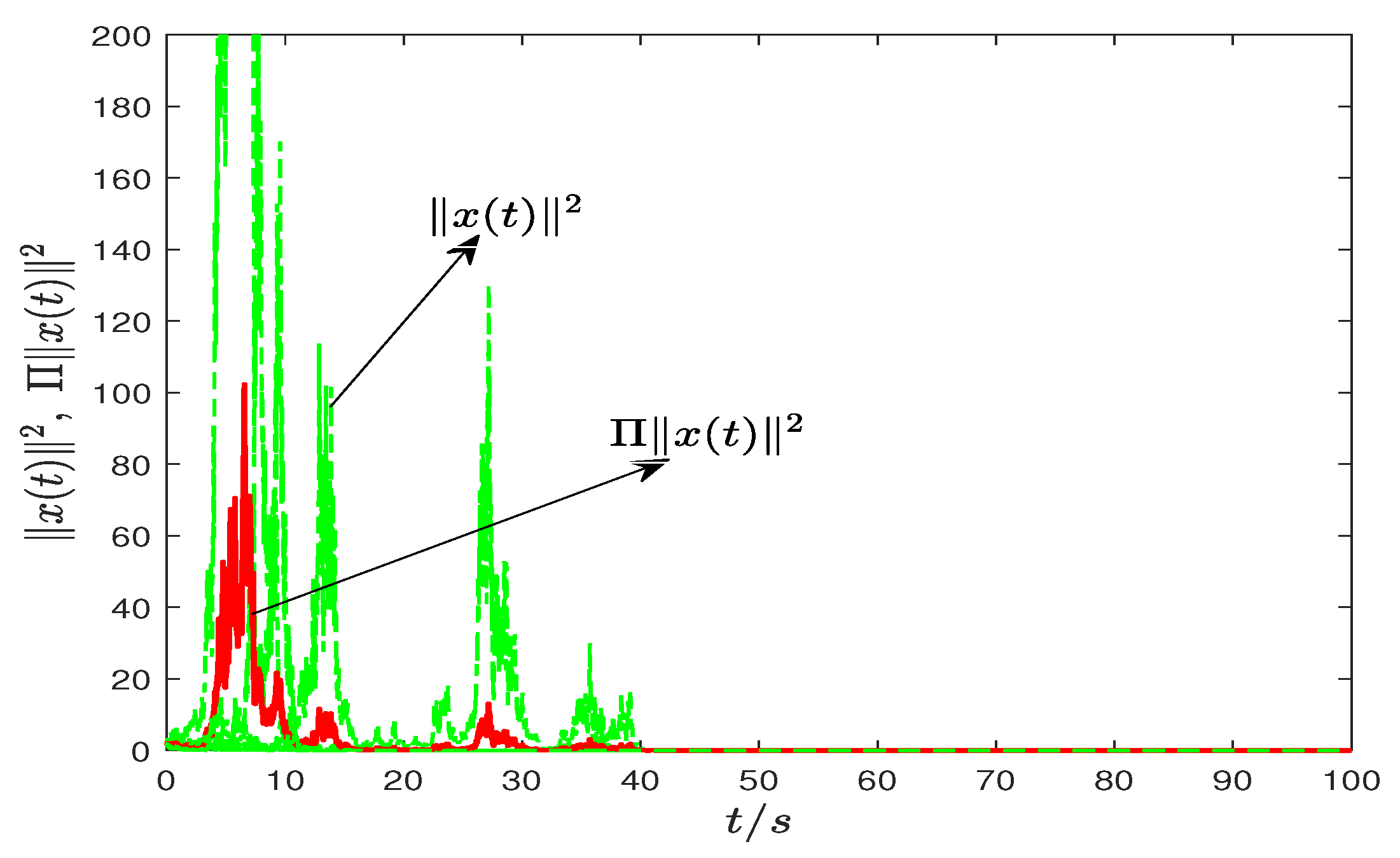
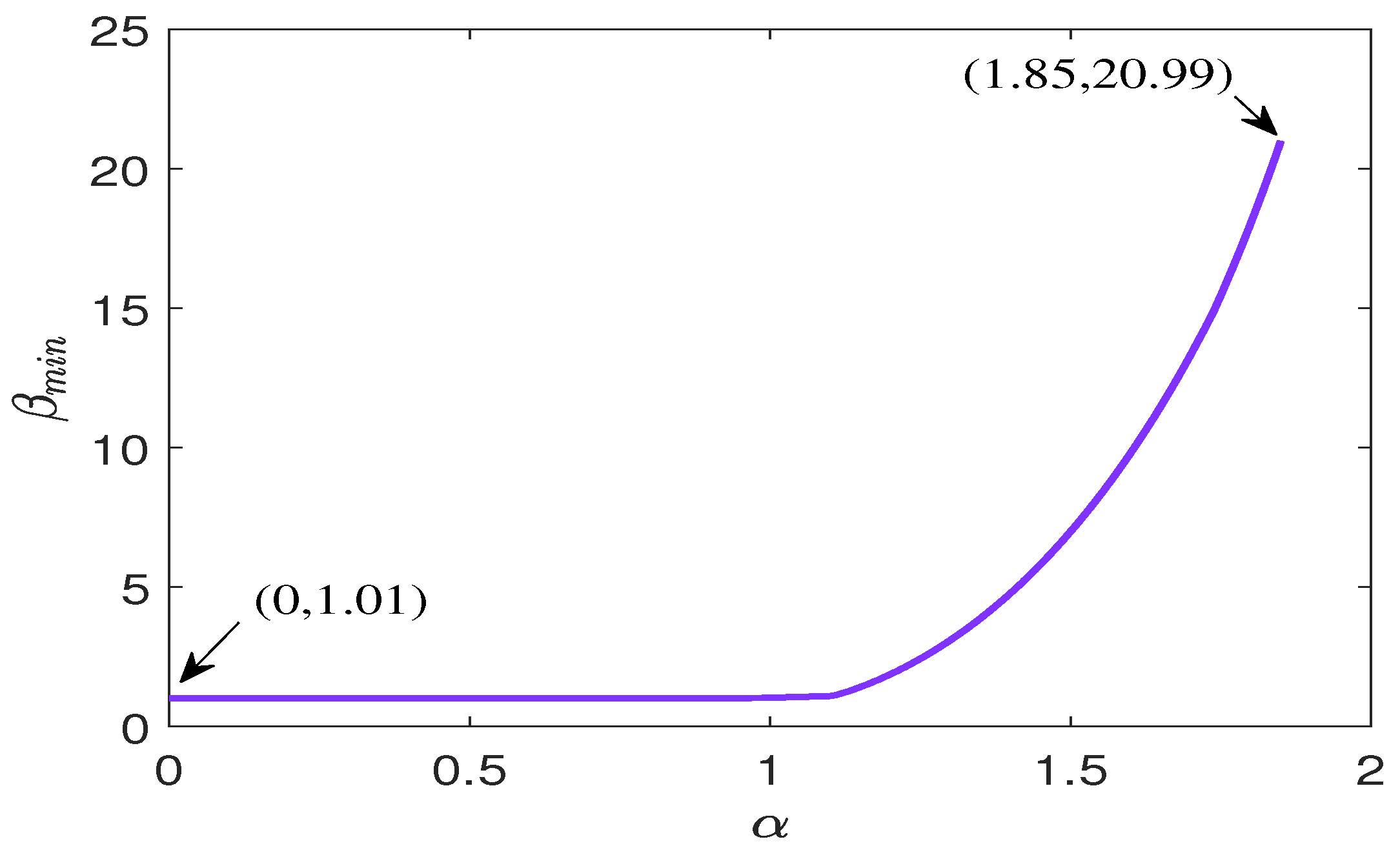
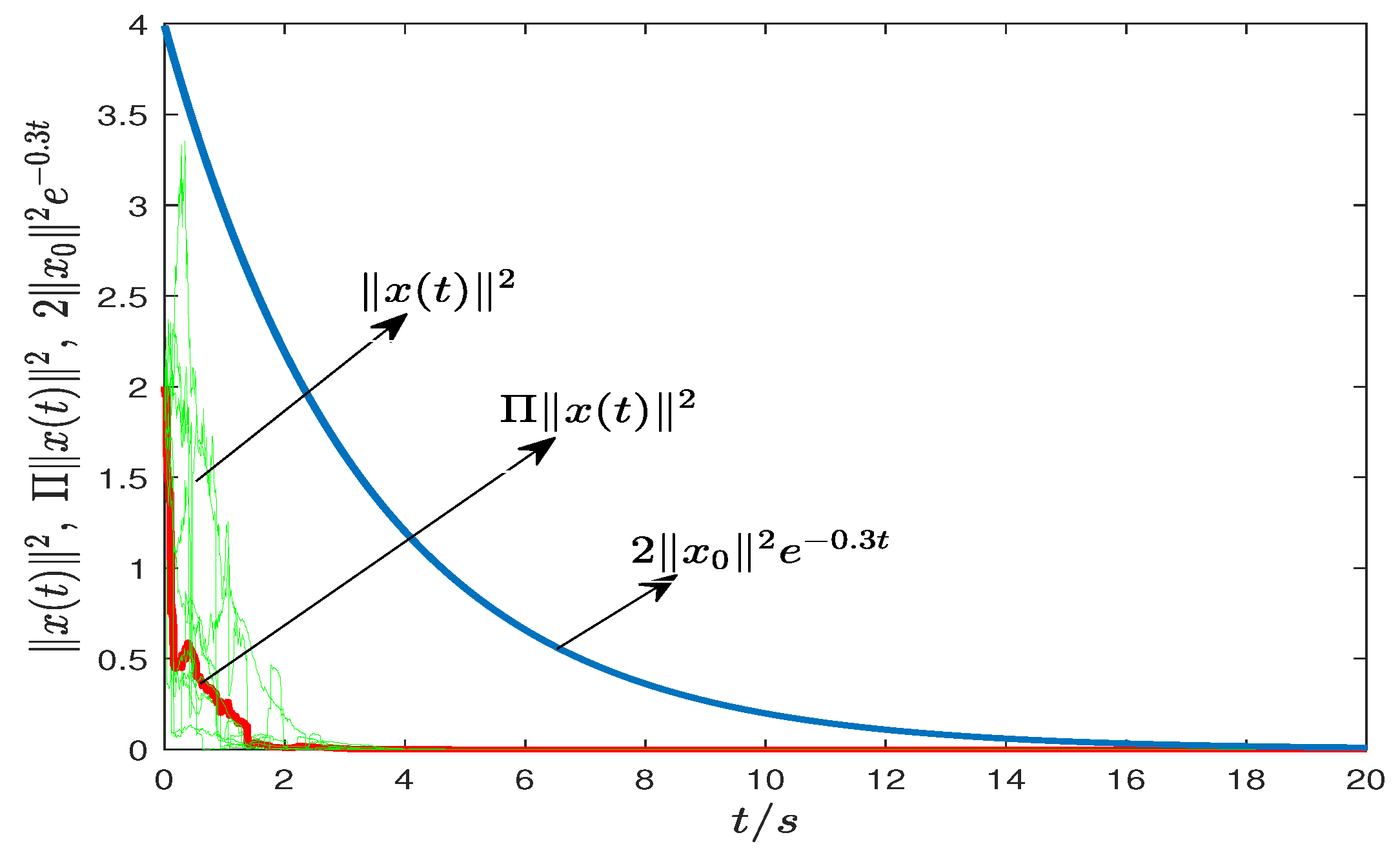
6.1. Example 1
- when ,
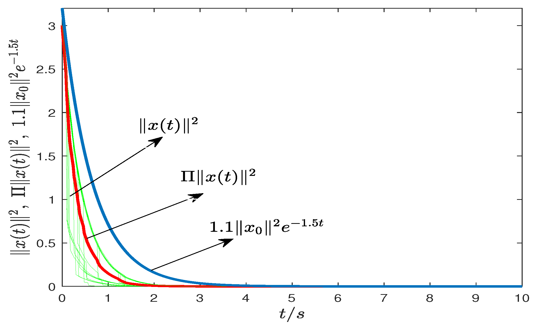
- when ,
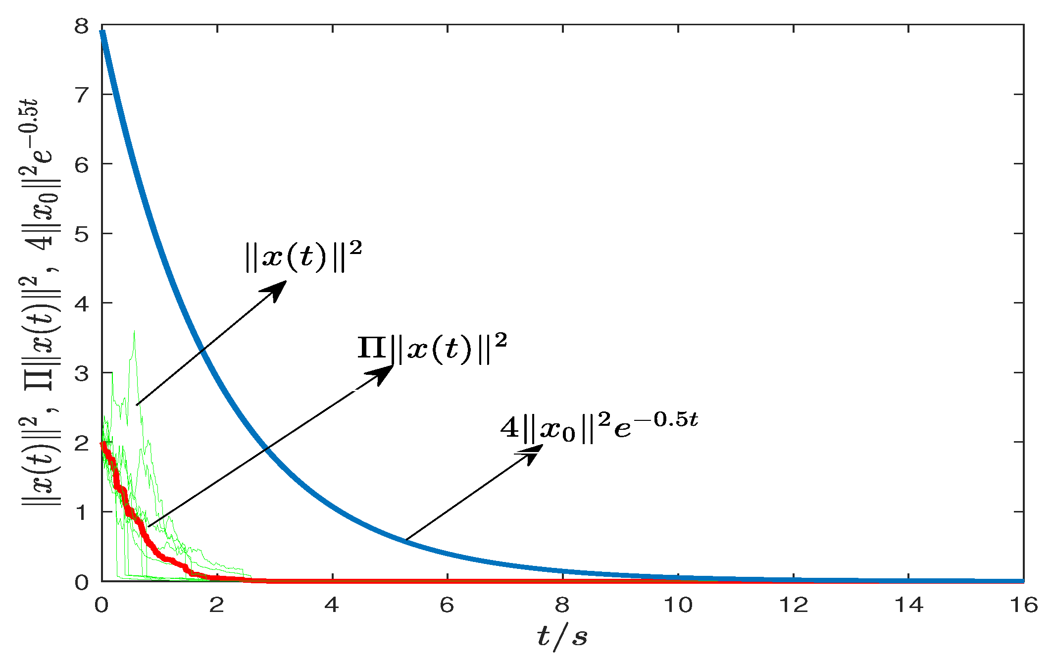
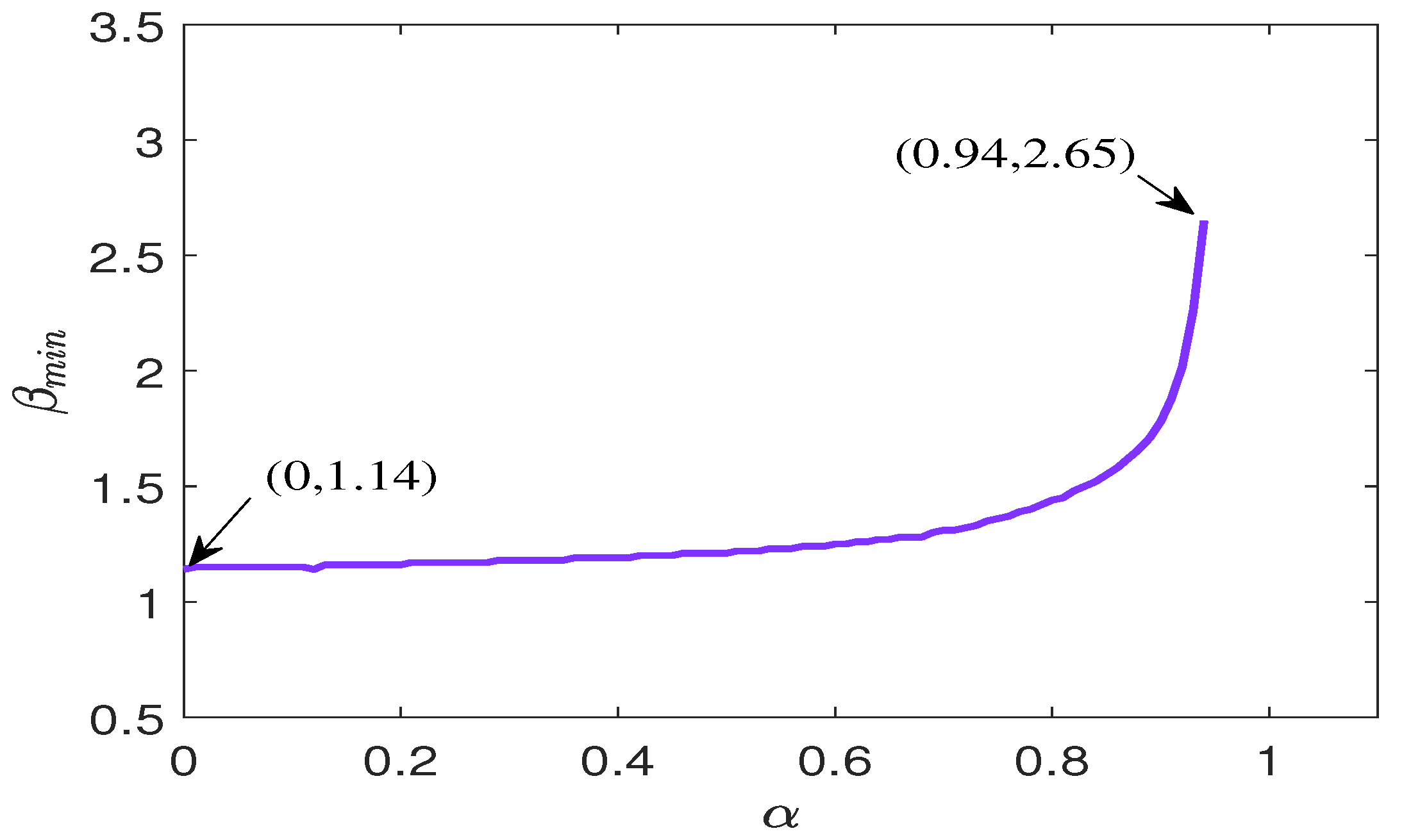
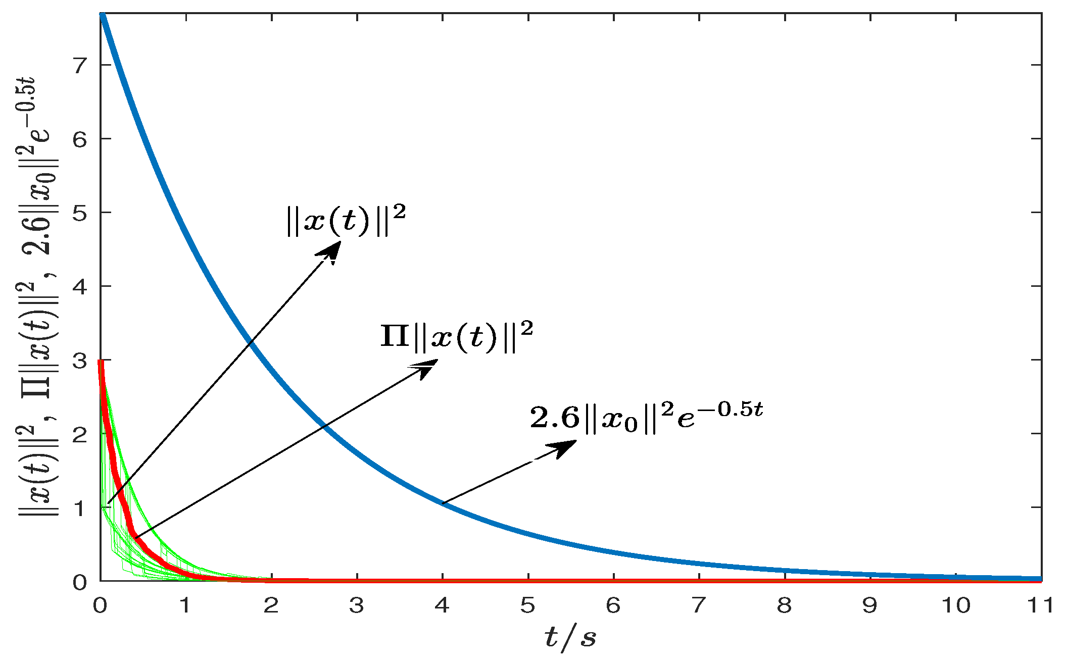
6.2. Example 2
7. Conclusions
Author Contributions
Funding
Institutional Review Board Statement
Informed Consent Statement
Data Availability Statement
Conflicts of Interest
References
- Zhang, G.L.; Song, M.H.; Liu, M.Z. Exponential stability of the exact solutions and the numerical solutions for a class of linear impulsive delay differential equations. J. Comput. Appl. Math. 2015, 285, 32–44. [Google Scholar] [CrossRef]
- Cai, T.; Cheng, P. Exponential stability theorems for discrete-time impulsive stochastic systems with delayed impulses. J. Frankl. Inst. 2020, 357, 1253–1279. [Google Scholar] [CrossRef]
- Cheng, P.; Deng, F.; Yao, F. Almost sure exponential stability and stochastic stabilization of stochastic differential systems with impulsive effects. Nonlinear Anal. Hybrid Syst. 2018, 30, 106–117. [Google Scholar] [CrossRef]
- Abedi, F.; Leong, W.J.; Shahemabadi, A.R. Exponential stability of some interconnected stochastic control systems with non-trivial equilibria. Eur. J. Control 2021, 58, 174–182. [Google Scholar] [CrossRef]
- Zhang, D.; Yu, L. Exponential stability analysis for neutral switched systems with interval time-varying mixed delays and nonlinear perturbations. Nonlinear Anal. Hybrid Syst. 2012, 6, 774–786. [Google Scholar] [CrossRef]
- Socha, L.; Zhu, Q. Exponential stability with respect to part of the variables for a class of nonlinear stochastic systems with Markovian switchings. Math. Comput. Simul. 2019, 155, 2–14. [Google Scholar] [CrossRef]
- Nguyen Khoa, S.; Le, V.N. Exponential stability analysis for a class of switched nonlinear time-varying functional differential systems. Nonlinear Anal. Hybrid Syst. 2022, 44, 101177. [Google Scholar] [CrossRef]
- Tran, K.Q.; Nguyen, D.H. Exponential stability of impulsive stochastic differential equations with Markovian switching. Syst. Control Lett. 2022, 162, 105178. [Google Scholar] [CrossRef]
- Yan, Z.; Song, Y.; Park, J. Quantitative mean square exponential stability and stabilization of stochastic systems with Markovian switching. J. Frankl. Inst. 2018, 355, 3438–3454. [Google Scholar] [CrossRef]
- Yan, Z.; Zhang, W.; Park, J.; Liu, X. Quantitative exponential stability and stabilization of discrete-time Markov jump systems with multiplicative noises. IET Control Theory Appl. 2017, 11, 2886–2892. [Google Scholar] [CrossRef]
- Cao, Z.; Niu, Y. Finite-time sliding mode control of Markovian jump systems subject to actuator nonlinearities and its application to wheeled mobile manipulator. J. Frankl. Inst. 2018, 355, 7865–7894. [Google Scholar] [CrossRef]
- Zhai, D.; An, L.; Li, J.; Zhang, Q. Fault detection for stochastic parameter-varying Markovian jump systems with application to networked control systems. Appl. Math. Model. 2016, 40, 2368–2383. [Google Scholar] [CrossRef]
- Kim, S.H. H2 control of Markovian jump LPV systems with measurement noises: Application to a DC-motor device with voltage fluctuations. J. Frankl. Inst. 2017, 354, 1784–1800. [Google Scholar] [CrossRef]
- Yan, Z.; Song, Y.; Liu, X. Finite-time stability and stabilization for Itô-type stochastic Markovian jump systems with generally uncertain transition rates. Appl. Math. Comput. 2018, 321, 512–525. [Google Scholar] [CrossRef]
- Guo, Y. Stabilization of positive Markov jump systems. J. Frankl. Inst. 2016, 353, 3428–3440. [Google Scholar] [CrossRef]
- Song, B.; Wu, Z.; Park, J. Filtering for stochastic systems driven by Poisson processes. Int. J. Control 2015, 88, 2–10. [Google Scholar] [CrossRef]
- Lin, X.; Zhang, R. H∞ control for stochastic systems with Poisson jumps. J. Syst. Sci. Complex. 2011, 24, 683–700. [Google Scholar] [CrossRef]
- Guo, Y.; Feng, J. Stabilization of stochastic delayed networks with Markovian switching via intermittent control: An averaging technique. Neural Comput. Appl. 2022, 34, 4487–4499. [Google Scholar] [CrossRef]
- Wu, Z.; Su, H.; Chu, J. H∞ filtering for singular Markovian jump systems with time delay. Int. J. Robust Nonlinear Control 2010, 20, 939–957. [Google Scholar] [CrossRef]
- Sun, T.; Su, H.; Wu, Z. State feedback control for discrete-time Markovian jump systems with random communication time delay. Asian J. Control 2014, 16, 296–302. [Google Scholar] [CrossRef]
- Chen, W.; Chen, B. Robust stabilization design for nonlinear stochastic system with Poisson noise via fuzzy interpolation method. Fuzzy Sets Syst. 2013, 217, 41–61. [Google Scholar] [CrossRef]
- Chen, B.; Wu, C. Robust scheduling filter design for a class of nonlinear stochastic poisson signal systems. IEEE Trans. Signal Process. 2015, 63, 6245–6257. [Google Scholar] [CrossRef]
- Lin, Z.; Liu, J.; Niu, Y. Dissipative control of non-linear stochastic systems with Poisson jumps and Markovian switchings. IET Control Theory Appl. 2012, 6, 2367–2374. [Google Scholar] [CrossRef]
- Yan, Z.; Zhou, X.; Ji, D. Finite-time annular domain stability and stabilisation of Itô-type stochastic time-varying systems with Wiener and Poisson noises. Int. J. Control 2021, 1–18. [Google Scholar] [CrossRef]
- Zhong, S.; Zhang, W.; Yan, Z. Finite-time annular domain stability and stabilization for stochastic Markovian switching systems driven by Wiener and Poisson noises. Int. J. Robust Nonlinear Control 2020, 31, 2290–2304. [Google Scholar] [CrossRef]
- Chen, G.; Sun, J.; Chen, J. Mean square exponential stabilization of sampled-data Markovian jump systems. Int. J. Robust Nonlinear Control 2018, 28, 5876–5894. [Google Scholar] [CrossRef]
- Yan, Z.; Zhang, G.; Zhang, W. Finite-time stability and stabilization of linear Itô stochastic systems with state and control-dependent noise. Asian J. Control 2013, 15, 270–281. [Google Scholar] [CrossRef]


Publisher’s Note: MDPI stays neutral with regard to jurisdictional claims in published maps and institutional affiliations. |
© 2022 by the authors. Licensee MDPI, Basel, Switzerland. This article is an open access article distributed under the terms and conditions of the Creative Commons Attribution (CC BY) license (https://creativecommons.org/licenses/by/4.0/).
Share and Cite
Chang, G.; Sun, T.; Yan, Z.; Zhang, M.; Zhou, X. Quantitative Mean Square Exponential Stability and Stabilization of Linear Itô Stochastic Markovian Jump Systems Driven by Both Brownian and Poisson Noises. Mathematics 2022, 10, 2330. https://doi.org/10.3390/math10132330
Chang G, Sun T, Yan Z, Zhang M, Zhou X. Quantitative Mean Square Exponential Stability and Stabilization of Linear Itô Stochastic Markovian Jump Systems Driven by Both Brownian and Poisson Noises. Mathematics. 2022; 10(13):2330. https://doi.org/10.3390/math10132330
Chicago/Turabian StyleChang, Gaizhen, Tingkun Sun, Zhiguo Yan, Min Zhang, and Xiaomin Zhou. 2022. "Quantitative Mean Square Exponential Stability and Stabilization of Linear Itô Stochastic Markovian Jump Systems Driven by Both Brownian and Poisson Noises" Mathematics 10, no. 13: 2330. https://doi.org/10.3390/math10132330
APA StyleChang, G., Sun, T., Yan, Z., Zhang, M., & Zhou, X. (2022). Quantitative Mean Square Exponential Stability and Stabilization of Linear Itô Stochastic Markovian Jump Systems Driven by Both Brownian and Poisson Noises. Mathematics, 10(13), 2330. https://doi.org/10.3390/math10132330