Abstract
The propagation of nonlinear water waves under complex wave conditions is the key issue of hydrodynamics both in coastal and ocean engineering, which is significant in the prediction of strongly nonlinear phenomena regarding wave–structure interactions. In the present study, the meshless generalized finite difference method (GFDM) together with the second-order Runge–Kutta method (RKM2) is employed to construct a fully three-dimensional (3D) meshless numerical wave flume (NWF). Three numerical examples, i.e., the propagation of freak waves, irregular waves and focused waves, are implemented to verify the accuracy and stability of the developed 3D GFDM model. The results show that the present numerical model possesses good performance in the simulation of nonlinear water waves and suggest that the 3D “RKM2-GFDM” meshless scheme can be adopted to further simulate more complex nonlinear problems regarding wave–structure interactions in ocean engineering.
Keywords:
meshless method; generalized finite difference method; nonlinear water waves; numerical wave flume; transient extreme waves; irregular waves; focused waves MSC:
76M10
1. Introduction
Over the past several decades, extensive extreme wave events have been observed both in coastal and ocean zones [1,2]. Extreme wave events, characterized by their randomness and unpredictability, are often the cause of destruction of ocean vehicles and floating platforms. Because such phenomena frequently threaten the safety of maritime staff and ocean engineering structures, their generating mechanisms deserve attention from both the scientific and industrial communities [3,4]. At present, physical experiments and numerical techniques have been widely employed to reproduce extreme wave events. However, it is well known that experiments are usually expensive and the reproducing of some extreme sea conditions in laboratories could be rather difficult. Therefore, numerical techniques, also known as computational fluid dynamics (CFD), can be a more feasible tool to tackle such problems.
In recent years, meshless methods for solving partial differential equations (PDEs), such as radial basis function (see, for example, [5]), smoothed particle hydrodynamics (see, for example, [6,7,8,9,10,11,12]), and the generalized finite difference method (see, for example, [13,14,15,16,17,18]) were developed significantly to deal with the disadvantages of traditional Eulerian mesh-based methods. Regarding the disadvantages, for example, in mesh-based methods, accurately capturing a water surface (or multiphase interfaces) is not trivial because of their mass non-conservation property. However, in meshless methods, the evolution of a free surface can be naturally fulfilled due to their inherent Lagrangian nature. Among various meshless methods, the generalized finite difference method (GFDM), a truly mesh-free and domain-type numerical method, was proposed by Benito et al. in 2001 [13].
In recent years, the GFDM has attracted more and more attention in practical applications for hydrodynamic problems. Zhang et al. [15] simulated the two-dimensional (2D) sloshing behaviors using the GFDM in combination with the explicit Euler method (EEM) and the semi-Lagrangian approach (SLA) under external horizontal and vertical excitations. It was found that although the “EEM-GFDM” model can greatly simulate the sloshing phenomena, some other time integration schemes can be considered in future studies. The main reason is that in the EEM, the time step size is required to be rather small to ensure numerical stability [15]. Given this reason, the EEM is unsuitable for solving complex engineering problems, where the computational costs can be a critical point for engineers. In order to tackle this issue, the second-order Runge–Kutta method (RKM2) was employed to investigate the propagation of nonlinear water waves in a 2D GFDM-based numerical wave flume (NWF) by Zhang et al. [14]. It was demonstrated that the “RKM2-GFDM” scheme holds better accuracy and stability for solving free-surface problems. These are the first two practical applications of the GFDM in ocean engineering, which suggests that the “RKM2-GFDM” scheme is a feasible tool for simulating ocean engineering problems. After that, the “RKM2-GFDM” scheme was successfully employed to investigate more complicated hydrodynamic issues, such as 2D shallow water problems [19], wave–current interactions [20], Boussinesq-type equations [21], and hydrodynamics loads acting on an offshore structure [16]. The GFDM was also modified by Fu et al. [18] into an advanced format by employing two truncated treatments, i.e., the so-called absorbing boundary conditions (ABC) and perfectly matched layer (PML). It was demonstrated that the new scheme can accurately simulate the wave–structure phenomenon of single- and four-cylinder array bodies.
More recently, the GFDM [14] was further improved from 2D to fully 3D formalism for simulating nonlinear water waves in ocean engineering, such as first-order waves, second-order Stokes waves and wave–structure interactions [17]. It was distinctly demonstrated that the 3D version is better than the 2D one for simulating the evolution of nonlinear water waves. Nevertheless, in the previous studies, such as those of Zhang et al. [14] and Huang et al. [17], some critical types of nonlinear water waves, such as freak waves, irregular waves and focused waves, were not involved. In fact, such water waves were already successfully simulated via other mesh-free schemes, such as smoothed particle hydrodynamics (SPH) (see, for example, [22,23]), whereas to the best knowledge of the authors, there has been no work on simulating these complex water waves based on the GFDM. In the present study, we aim at shedding light on this topic within the GFDM framework. This paper can be treated as a further improvement of the pre-developed GFDM-based NWF [14,17,20]. The remainder of this paper is arranged as follows. In Section 2, the governing equations as well as boundary conditions of the 3D GFDM-based NWF are elaborated mathematically. In Section 3, the meshless scheme dealing with the spatial variables of the deformable computational domain is introduced in detail. In Section 4, three numerical benchmarks involving transient extreme waves, two types of irregular waves, and focused waves are investigated to verify the accuracy and stability of the proposed 3D GFDM model.
2. Governing Equations and Boundary Conditions of the 3D GFDM Scheme
In the present study, a rectangular NWF is developed based on the 3D GFDM model for predicting the evolution of nonlinear water waves under complex wave conditions. As is shown in Figure 1a, the origin of a Cartesian coordinate system is considered at the bottom corner of the NWF. The undisturbed water depth, length and width of the NWF are respectively denoted by h, b, and w. All boundary conditions of the developed NWF are divided into five parts, including the upstream, downstream, bottom, side, and free-surface boundaries, which are also denoted by , , , and , respectively.
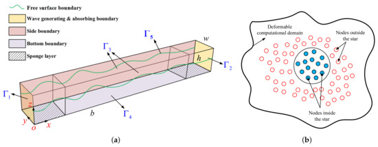
Figure 1.
Schematic diagram of the developed 3D GFDM-based NWF. (a) Boundary conditions of the 3D GFDM-based NWF. (b) Nodes and the star in the GFDM.
2.1. Governing Equations
It is assumed that the flow field in the NWF is inviscid, incompressible, and irrotational, which means that the potential flow theory can be employed to describe the fluid behaviors in the present study. Consequently, the 3D Laplace’s equation for the velocity potential is given as
where is the velocity potential, and denotes the whole flow field.
2.2. Free-Surface Boundary Condition
The kinematic and dynamic boundary conditions are implemented to describe the dynamic evolution of free-surface elevation, which yield
where denotes the water surface elevation and is vertically evaluated above the undisturbed water level , g is the acceleration of gravity, and is the kinetic energy of fluid particles given as
The kinematic boundary condition Equation (2) states the fact that no fluid particles can penetrate the free surface. Furthermore, the dynamic boundary condition Equation (3) denotes the fact that the pressure on the free surface is uniformly distributed along with the z-axis direction and should be equal to zero (i.e., atmospheric pressure).
2.3. Bottom and Side Boundary Conditions
The impermeable bottom and side boundaries of the computational domain should satisfy the no-flux condition, which means that the fluid particles cannot penetrate these surfaces and thus yield
where is the unit normal vector along with the wall boundary (outward).
2.4. Upstream Boundary Condition
In the following calculations, all incident water waves are generated using a piston-type wavemaker to reproduce the desired complex ocean environments, which means that the wave-making boundary can be realized by enforcing a horizontal velocity such that
where is the velocity function, which can be derived under different physical conditions (see Section 4). According to our previous investigation [14], the incident water waves should be produced via a ramping function to ensure the robustness of the numerical simulations. In the present study, is considered as
where is the modulation time depending on the mathematical form of velocity function. As a result, the wave-making boundary condition should be recast as
2.5. Downstream Boundary Condition
At the end of the NWF, a numerical beach must be employed to absorb the wave energy. In the present study, the Sommerfeld–Orlanski radiation boundary condition in combination with a sponge layer [14] is carried out to avoid numerical instability due to the phenomenon of the wave reflection, which means that the downstream boundary condition can be expressed as
Since a numerical beach is deployed to tackle the wave reflection at the downstream boundary, the kinematic and dynamic conditions of the water surface are rewritten as
in which
where is the damping coefficient for the sponge layer, is the angular wave frequency, is the length factor, and is the tuning factor of the sponge layer.
After the detailed illustrations of the mathematical formulations of the developed 3D GFDM-based NWF, it can be summarized that the governing equation for the whole flow field is Laplace’s equation, Equation (1); the time-dependent free-surface boundary satisfies the kinematic and dynamic conditions, Equations (2) and (3); and the bottom, side, upstream and downstream boundaries are governed by the Neumann boundary conditions, Equations (5), (8) and (9), respectively. It is obvious that the introduced governing equation and boundary conditions yield an initial-boundary value problem, which is discretized numerically by the 3D “RKM2-GFDM” meshless scheme elaborated in the following section.
3. Numerical Methods
In the previous section, the initial-boundary value problem for the NWF is yielded based on the potential flow theory with a full Lagrangian description. In this section, the RKM2 in conjunction with the SLA is employed as the time-integration scheme, while the GFDM is adopted to discretize the spatial variables .
3.1. Temporal Discretization
In order to prevent the computational nodes from escaping out of the deformable flow field, the full Lagrangian description Equations (10) and (11) are thus modified with the SLA [14,20]. According to the numerical procedures of the SLA, the freedom of the fluid particles at the free surface () is frozen except for the z-axis direction, which yields
where is the vertical velocity at the free surface, and is the material derivative. Substituting and into the material derivative operator yields the following expressions:
According to Equations (14) and (15), the semi-Lagrangian description of Equations (10) and (11) can be re-written as
Considering the better numerical stability, the RKM2 scheme is employed to discretize Equations (16) and (17). At the beginning of a simulation, the derivatives and can be evaluated via the free-surface boundary conditions, and the marching scheme regarding the time integration of and can be expressed as
where the superscripts n and ∗ refer to the field quantities at and the temporary time step, respectively. After the temporary field quantities are derived, the time derivative at can be evaluated after reconstructing the particles along every vertical line. The numerical process can be marched into the next time layer in the same manner, and the field quantities at can be given as
3.2. Spatial Discretization
On the basis of the GFDM, the so-called moving-least-squares method is adopted to approximate the spatial derivatives for every node at each time step by solving a linear–combined sparse system. In order to briefly introduce the meshless scheme, as is shown in Figure 1b, a point cloud can be found within a certain region in the deformable computational domain. Assuming that the i-th node is an arbitrary node within the selected region, nearest nodes in the proximity of the i-th node can be defined to form a support domain. The shapes of the support domain can be given in different choices [13,24]. In the present study, a circular support domain is adopted for the sake of simplicity. Once the support domain for the i-th node is defined, the Taylor series truncated by the second-order derivative is then employed to re-formulate the governing equation inside the support domain. Therefore, it is possible to define the function according to the moving-least-squares method, which yields
where and are field quantities at the i-th node and other nearest nodes; , , and are the distances between the i-th node and the j-th node in the support domain along with the x-, y-, z axes. represents the so-called weighting function and is considered the quadratic spline [13] in the present study such that
where is the distance between the i-th node and the j-th node of the support domain, is the distance between the i-th node and the farthest node within the star. Because Equation (22) represents the weighted residual of the Taylor series approximation within the support domain, it is natural to expect that the norm can be minimized regarding a partial derivative vector such that
where
A linear system of algebraic equations is thus yielded,
where
It is obvious that matrix is symmetric. Matrix can be recast as
where is the field quantities at the i-th nodes and other nearest nodes within the support domain. represents a coefficient matrix. The specific value of the matrix depends on the spatial coordinate and weighting function of the node within the support domain of the i-th node. As a result, can be re-written as
where is the coefficient matrix depending on the weighting function, the numbers of nodes within the support domain and the spatial coordinates of nodes within the star. For the sake of clarity, the above equation can be recast as
where are weighting coefficients with respect to the nodes and the support domain, which can be numerically calculated using the above developed numerical method. Because the i-th node depicted above is arbitrarily selected in the deformable computational domain without any assumptions, it is obvious that every node both at the interior and boundary should be considered the i-th node to derive the derivatives expression by repeating the pipeline of Equations (22)–(30). Consequently, a linear algebraic system of physical values with different weighting functions is formed by transforming the spatial derivative at the i-th node. It is obvious that the GFDM is easy to code and very efficient due to the merits of the sparse matrix. For the sake of clarity, in Figure 2, a flowchart regarding the implementation of the present GFDM model is displayed.
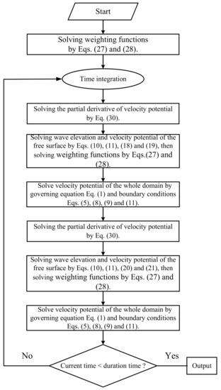
Figure 2.
The flowchart of the present GFDM model.
It should be underlined that the size of the support domain (i.e., the number of neighbors of each point) contributes to the numerical accuracy of the GFDM model. However, it also affects the computational costs of simulations. In order to test the required CPU time for different numbers of neighbors, a benchmark is performed, and the final result is listed in Table 1. One can see that the required time per time step increases with the increase in neighbors. As highlighted in the previous work [17], can be enough for the simulations of nonlinear water waves propagation, whereas in the present study, is adopted to better capture the free-surface evolution.

Table 1.
The computational costs per time step with respect to different local-domain sizes.
In the following section, three numerical examples with respect to the transient extreme waves, two types of irregular waves, as well as the focused waves are investigated, discussed and compared with other results to verify the accuracy and stability of the present numerical model.
4. Examples Implementation and Discussion
4.1. Example 1: Transient Extreme Waves
Transient extreme waves are strong nonlinear fluid behaviors characterized by their extraordinarily large wave height, which can be the main cause of many accidents of fixed and floating offshore structures. In practical engineering, transient extreme waves play an important role in the hydrodynamics of marine vessels encountering green water or wave overtopping events. In this numerical example, we reproduce the transient extreme wave using the same method adopted by [25]. In their physical experiment, a short transient extreme wave was chosen because the investigation of the kinematics of one wave overtopping on deck event requires a large number of repeated runs. In our developed 3D GFDM-based NWF, a short transient extreme wave is generated by giving the wave-making boundary a pre-designed piston signal [25]. As is shown in Figure 3, the piston signal contains two cycles of a sinusoidal wave with amplitude followed by two and a half cycles of a sinusoidal wave with larger amplitude . The velocity function U produced via the piston-type wavemaker is written as
where H is the wave height, k is the wavenumber, d is the water depth, and is the angular wave frequency. Figure 4 shows the schematic diagram of Example 1. The length b, width w and depth h of the NWF are adopted as 24.0, 0.1 and 0.65 m, respectively. The upstream boundary is considered the wave-making condition with imposing horizontal velocity generated by the above-mentioned piston signal, while the downstream boundary is adopted as the wave-absorbing condition to tackle the wave reflection with length factor and tuning factor . In order to implement a benchmark of the studied numerical example, as shown in Figure 4, the wave elevation is measured using 15 wave gauges beginning at from the upstream boundary and continuing in increments of 0.5 m to . In this numerical example, the time step, numbers of nodes for whole computational domain and within the star are set with , , and , respectively. The duration time t of the simulation process is adopted as .
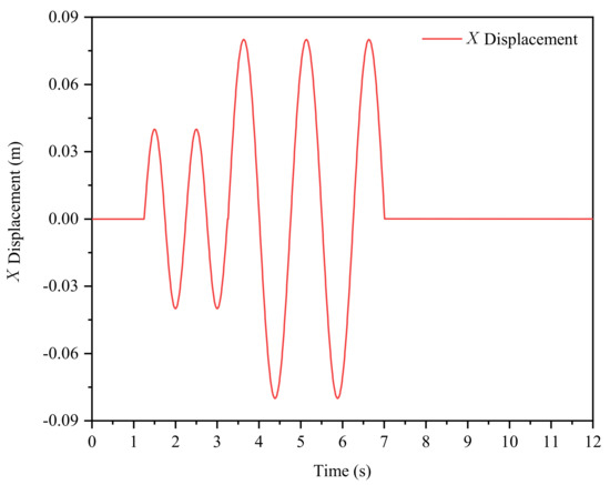
Figure 3.
Profile of the piston signal given to the wave-making boundary for Example 1, which starts from and ends at .
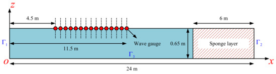
Figure 4.
Schematic diagram of the 3D GFDM-based NWF employed for Example 1.
As is shown in the experiment investigated by [25], the transient nature of the tests, evidently, can be divided into three states. Initially, two large waves exist at , which are then transformed into a single and larger wave at . Finally, the focused wave decomposes into two large waves at . Figure 5 shows the comparison between the numerical and experimental results at , , , respectively. Figure 6 depicts the shape of the free surface at the moment when the maximum wave height appears. It is illustrated that the numerical results derived from the developed 3D GFDM-based NWF are in good agreement with the physical experiment results, which demonstrates that the newly developed numerical method can accurately capture the focusing phenomenon of water waves.
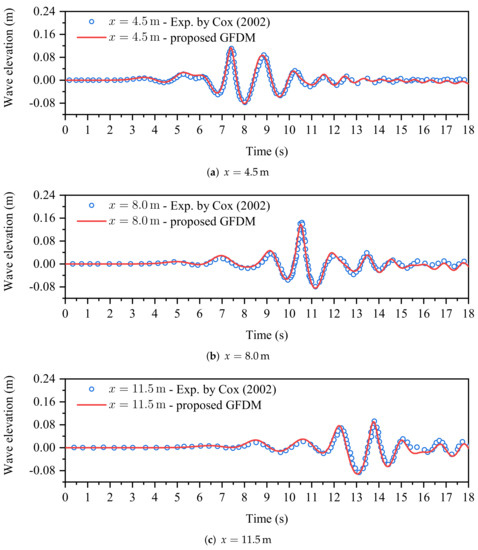
Figure 5.
Comparison between numerical and experimental results at x = 4.5 m, 8.0 m, 11.5 m.
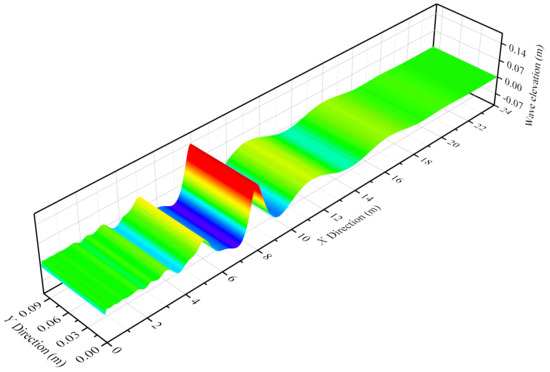
Figure 6.
Shape of free surface at the moment when the maximum wave height appears.
In order to further verify the effectiveness and accuracy of the 3D GFDM-based NWF, the monitored maximum wave height and their respective corresponding time of every employed wave gauge are listed in Table 2 in which the experimental results and the relative error are also included as a comparison. It can be observed that the simulated maximum wave height at different wave gauges and their respective corresponding time are also in good accordance with the experimental results. As for the maximum wave height, the maximum relative error is at the location of . The average of the relative error with respect to the maximum wave height exceeds no , which is accurate, generally, for practical engineering applications. As is shown in Table 2, the corresponding time of the occurrence of the maximum wave height is greatly captured and is almost identical to the experimental data. The maximum relative error of the corresponding time is , and the average of the relative error does not exceed . In fact, in the present study, the viscosity and turbulence effects are neglected in total because the present GFDM is based on the potential flow model. However, in the experiments, the viscosity and turbulence effects can be taken into account. For this reason, one can see that the errors of wave heights are somewhat greater than those of time. Despite this, the maximum error is below 7%, which is acceptable in engineering applications. Of course, in the future, we will further improve our GFDM model by solving the Navier–Stokes equation instead of Laplace’s equation, and we believe that through this consideration, the numerical accuracy can be further improved. On the whole, from the above discussions, it is demonstrated that the proposed 3D meshless scheme shows satisfactory accuracy in the prediction of transient extreme waves.
Table 2.
Comparison of the maximum wave height and respective corresponding time between numerical and experimental results.
4.2. Example 2: Irregular Waves
In recent years, the GFDM has been successfully carried out for many practical engineering problems, such as water wave propagations and wave–current interactions [14,20], BTEs (Boussinesq-type equations) [21], and first-order water wave interactions with ocean and offshore structures [18], in which the incident water waves are employed in a monochromatic type. Nevertheless, there is no work relating to the applications of irregular waves using the GFDM. The actual sea surface consists of waves with different directions, frequencies, phases and amplitudes. For an accurate description of the real ocean environment, a large number of waves must be superimposed. In this numerical example, two types of irregular waves are simulated based on the proposed 3D meshless scheme. One of them is a typical form using the JONSWAP (Joint North Sea Wave Project) spectrum. Another one is the so-called white noise irregular water waves, which is always employed in physical experiments for the hydrodynamic performance of floating offshore structures to obtain the response amplitude operators (RAOs) under different wave frequencies.
4.2.1. JONSWAP Spectrum
In the present study, the traditional Longuet–Higgins model [26] is employed to describe the irregular wave elevation such that
where , , , , and denote the wave amplitude, wave number, propagating direction, angular wave frequency and random phase angle of the i-th wave component, respectively. The random phase angles are homogeneously distributed between 0 and and are constant with time. The wave amplitude can be obtained by giving a wave spectrum such that
where and are constant differences of successive frequencies and propagating directions, respectively. In the present study, the propagating direction of irregular waves is considered along the positive x-axis, resulting in , which means that Equations (41) and (42) can be recast as
and
The instantaneous wave elevation satisfies the Gaussian distributed with zero mean and variance equal to , which can be re-formulated using the mathematical definition of mean value and variance applied to a signal function represented by Equation (41). Consequently, the JONSWAP spectrum recommended by the International Towing Tank Conference [27] is adopted to express the such that
where
and
where is the significant wave height defined as the mean of the one-third highest waves. is the average period and can be derived by , with and being the spectral peak period and the average zero crossing period, respectively. In the present study, we define chosen from a sea-states table suggested by the International Association of Classification Societies (IACS) [28], which is the most frequent combination of real wave conditions. In the following simulation, the chosen significant wave height and the average zero crossing period are transformed into by the Froude law with scale 1:30. Finally, the selected and are thus derived as 0.03 m and , respectively. From the above discussions, the velocity function U in this numerical example can be given as
In this numerical example, the schematic diagram is the same as Figure 4. The depth h of the NWF is , while other geometry parameters of the NWF are consistent with Example 1. The time step and numbers of nodes for the whole computational domain and within the star are adopted with , , and , respectively. It is worth noting that the duration time t must be long enough to reflect the statistical characteristics of irregular waves. Consequently, the duration time t is considered with , which is approximately equivalent to 73 times the average zero-crossing wave period and is acceptable for the following spectrum analysis.
Figure 7 depicts the simulation results of the JONSWAP case. It can be observed from Figure 7a that the wave elevation shows random and irregular characteristics over time and are in good agreement with the theoretical solution. In order to further benchmark the accuracy of the numerical results, the fast Fourier transform (FFT) technique is carried out to implement a spectrum analysis of the time history curve. Figure 7b shows the comparison between the target spectrum and the simulated spectrum for the time slice. It can be seen that the simulated spectrum is basically in accordance with the target spectrum except for the location of the peak. As is shown in Figure 7b, the peak value of the simulated spectrum is slightly shifted to the lower frequency band compared with the target spectrum, which may be caused by the so-called spectrum leakage effect due to the rectangular window function. In general, the developed 3D meshless scheme shows good performance in such problems.
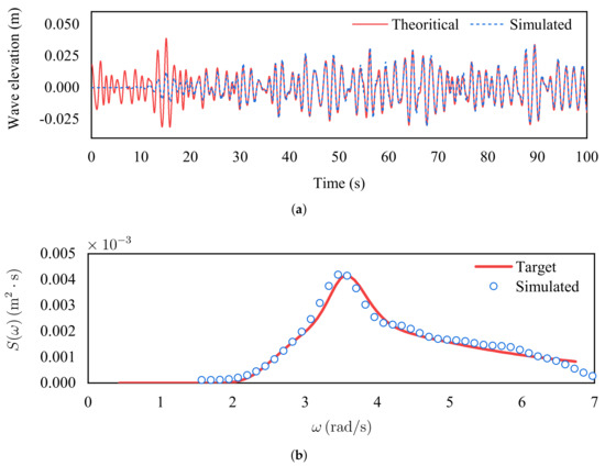
Figure 7.
Simulation results of the JONSWAP case (color figure available online). (a) Profile of the wave elevation monitored by the wave gauge at . (b) Comparison between the target spectrum and the simulated spectrum.
4.2.2. White Noise Spectrum
The above-mentioned JONSWAP spectrum is a typical narrow-band spectrum, which means that the energy of the JONSWAP spectrum is mainly concentrated near the peak frequency and rapidly attenuates to both sides with the peak frequency as the center. However, for a white noise spectrum, the most important feature is that the energy is a horizontal straight line in the desired frequency range. In this numerical case, the desired truncated low- and high-wave frequencies are chosen as and , respectively. The schematic diagram of the NWF and the numerical parameters , N, and t are the same as the JONSWAP case.
Figure 8 shows the simulation results of the white noise spectrum case. Similar to the previous case, it can be observed from Figure 8a that the time history curve also reflects the characteristics of irregular waves. The FFT technique is adopted again to derive the simulated spectrum, and the results are illustrated in Figure 8b. It can be observed that the amplitude of the simulated spectrum fluctuates slightly near the horizontal straight line in the target band. In the theoretical aspect, the white noise spectrum is an ideal mathematical model. However, there is unexpected noise existing in the physical experiments, aroused by the environmental complexity, and in computer simulations caused by some numerical noise, such as artificial dissipation, unreasonable time step or nodes resolution. In other words, it is almost impossible to obtain a perfect white noise spectrum neither in physical experiments nor in numerical simulations. Overall, the deviation shown in Figure 8b is acceptable and basically meets the needs of practical engineering applications. From the above discussions, it is demonstrated that the proposed 3D meshless scheme shows good performance for capturing the irregularity of water waves by giving a target spectrum.
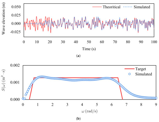
Figure 8.
Simulation results of the white noise spectrum case. (a) Profile of the wave elevation monitored by the wave gauge at . (b) Comparison between the target spectrum and simulated spectrum.
4.3. Example 3: Focused Waves
In Section 4.1, the focusing phenomenon of several components of water waves is observed by giving two cycles of a sinusoidal wave followed by two and a half cycles of a sinusoidal wave at the wave-making boundary . In real wave conditions, however, the wave elevation is more complicated and difficult to be predicted, especially for freak waves or rough waves. It is imperative to introduce a more effective model for describing the complexity of the actual ocean environments. The previous example demonstrates that the newly developed meshless scheme has good performance in the prediction of irregular waves. In this numerical example, the developed 3D GFDM-based NWF in Section 4.2 is employed again to simulate the focusing behavior of a series of monochromatic waves using the JONSWAP spectrum by controlling the phase angle for every wave component. Accordingly, the governing equations Equation (43) regarding the instantaneous wave elevation should be modified as
where and represent the focusing location and time, respectively. At the instant of , the crest of all wave components focuses at the location of , resulting in a focused wave characterized by its considerable wave crest. Consequently, the velocity function U is thus expressed as
For the sake of verifying the accuracy of the proposed 3D meshless scheme, a physical experiment [29] is reproduced by a numerical simulation based on the developed 3D GFDM-based NWF. In this numerical case, the focused waves are generated under the same experimental conditions using a constant wave amplitude (CWA) spectrum. The focusing location and focusing time are considered as and , respectively. Furthermore, the wave frequency band and the number of wave components are adopted as 5.236–7.854 rad/s and with the focusing wave amplitude being 0.022 m. In this numerical case, the geometry parameters of the NWF is employed the same as the physical wave flume [29], and the time step, numbers of nodes for the whole computational domain and within the star are set with , , and , respectively. The duration time t of the simulation process is adopted as . Figure 9 displays the comparison of free-surface elevation at the focusing location between the numerical results and experimental data. It is demonstrated that the numerical results of the focusing time and focusing locations are both in good agreement with the experimental data. In general, the 3D GFDM-based NWF shows satisfactory accuracy in the prediction of focused waves.
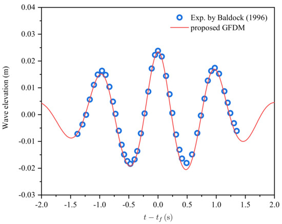
Figure 9.
Comparison of free-surface elevation at the focusing location between numerical results and experimental data.
In order to investigate the effects of the spectrum type for simulating focused waves using the 3D meshless scheme, three spectra (see Figure 10), including the JONSWAP spectrum, the CWA spectrum, and the constant wave steep (CWS) spectrum, are employed to generate three focused waves with identical numerical parameters, except for the spectrum type. The focusing location, focusing time, and focusing wave amplitude are adopted as , and , respectively. Figure 11a–c depicts the simulation results of three focused waves using the above-mentioned spectra. The shapes of the free surface at the focusing time for three spectra are also displayed in Figure 12. It can be observed that either the focusing time or the focusing location is in good accordance with the desired values for the three spectra. A comparison of three profiles for the wave elevation at the focusing location is shown in Figure 11d. In the initial stage of the numerical simulations, the free surface is very gentle, while it begins to fluctuate gradually as the calculation time continues to increase. After , the fluctuation of the free surface obviously becomes severe. Finally, at , the phenomenon of the wave focusing can be observed from the highest wave crest. Table 3 shows the comparison of the focusing location and the focusing time between the numerical results and designed values. It can be seen from the table that the focusing wave amplitude for the JONSWAP case is slightly over-predicted, with the error being , while the cases of CWA and CWS seem to be more accurate compared with the JONSWAP case. It is striking that the focusing time of three cases, as is shown in Table 3, are in great agreement with the designed values. From the above discussions of Table 2 and Table 3, it is demonstrated that the proposed 3D meshless scheme shows the great capability of capturing the focusing phenomenon of various monochromatic wave components.
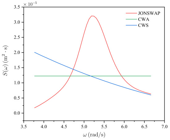
Figure 10.
JONSWAP, CWA and CWS spectrum given for the comparison study (color figure available online).
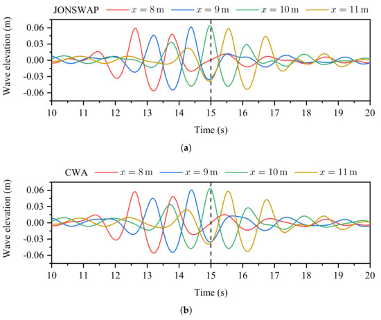
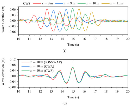
Figure 11.
Simulation results of the focused waves using JONSWAP, CWA and CWS spectra (color figure available online).(a) Time–history curves for the JONSWAP spectrum. (b) Time–history curves for the CWA spectrum. (c) Time–history curves for the CWS spectrum. (d) Time–history curves for the CWS spectrum.
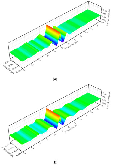
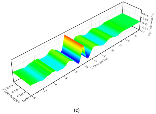
Figure 12.
The comparison of free surface between three spectra at the focusing time. (a) JONSWAP spectrum. (b) CWA spectrum. (c) CWS spectrum.
Table 3.
Comparison of the focusing wave amplitude and the focusing time between numerical results and designed values.
5. Conclusions
In the present study, we propose a 3D truly meshless scheme to investigate the dynamic behaviors of nonlinear water waves under complex wave conditions. Based on the potential flow hypothesis, the RKM2 in conjunction with the SLA is adopted to discretize the temporal variable of the 3D Laplace’s equation. At every time step, the spatial variables of the governing equation with mixed boundary conditions are solved, using the GFDM. The physical values at every computational node are transformed into a linear-combined algebraic system with different weighting coefficients and can be obtained efficiently due to the mathematical merits of the sparse matrix.
Three numerical examples are employed to verify the accuracy and stability of the present 3D GFDM model. In the first numerical benchmark, the transient extreme waves are reproduced by giving the wave-making boundary a piston signal with several sinusoidal wave components, and the phenomenon of transient extreme waves is successfully observed at a certain location. As for the second numerical example, two types of irregular waves are simulated using the JONSWAP spectrum and the white noise spectrum. The irregularity of the temporal evolution of the free surface is accurately calculated, and the simulated spectra are also in good agreement with the target spectra. Finally, the simulation of focused waves is carried out to predict the focusing phenomenon of various monochromatic wave components. Three spectra, including the JONSWAP, CWA and CWS spectra, are adopted to generate different irregular waves designed with the same focusing time and focusing location. The results show that the proposed 3D meshless scheme has the capability of capturing the phenomenon of waves focusing. In general, the newly developed 3D “RKM2-GFDM” meshless scheme shows great performance to predict the dynamic behaviors of nonlinear water waves under complex wave conditions. We underline that in the present study, the simulations are only considered in 2D formalism; the 3D effects will be further investigated. In the future, the hydrodynamic problem regarding the wave–structure interactions between freak waves and floating offshore structures will be numerically investigated based on the developed 3D GFDM-based NWF.
Author Contributions
Data curation, methodology, resources, software, validation, and writing—original draft preparation: J.H. Conceptualization, supervision, and writing—review and editing: C.-M.F. Funding acquisition and project administration: J.-H.C. Methodology and software: J.Y. All authors have read and agreed to the published version of the manuscript.
Funding
This research was funded by National Natural Science Foundation of China (Grant No. 52171346); Guangdong provincial special fund for promoting high quality economic development (Grant No. GDNRC[2021]56); Zhanjiang unfunded science and technology research project (Grant No. 2020B01415).
Institutional Review Board Statement
Not applicable.
Informed Consent Statement
Not applicable.
Data Availability Statement
Not applicable.
Conflicts of Interest
The authors declare no conflict of interest. This submitted manuscript has been approved by all authors for publication. We would like to declare that the work described is original research that has not been published previously, and is not under consideration for publication elsewhere, in whole or in part. The authors listed have approved the manuscript that is enclosed.
References
- Chien, H.; Kao, C.C.; Chuang, L.Z.H. On the Characteristics of Observed Coastal Freak Waves. Coast. Eng. J. 2002, 44, 301–319. [Google Scholar] [CrossRef]
- Nikolkina, I.; Didenkulova, I. Rogue waves in 2006–2010. Nat. Hazards Earth Syst. Sci. 2011, 11, 2913–2924. [Google Scholar] [CrossRef]
- Lavrenov, I.; Porubov, A. Three reasons for freak wave generation in the non-uniform current. Eur. J. Mech.-B/Fluids 2006, 25, 574–585. [Google Scholar] [CrossRef]
- Onorato, M.; Residori, S.; Bortolozzo, U.; Montina, A.; Arecchi, F. Rogue waves and their generating mechanisms in different physical contexts. Phys. Rep. 2013, 528, 47–89. [Google Scholar] [CrossRef]
- Nikan, O.; Avazzadeh, Z. An efficient localized meshless technique for approximating nonlinear sinh-Gordon equation arising in surface theory. Eng. Anal. Bound. Elem. 2021, 130, 268–285. [Google Scholar] [CrossRef]
- Monaghan, J.J. Smoothed particle hydrodynamics. Rep. Prog. Phys. 2005, 68, 1703–1759. [Google Scholar] [CrossRef]
- Liu, M.B.; Liu, G.R. Smoothed Particle Hydrodynamics (SPH): An Overview and Recent Developments. Arch. Comput. Methods Eng. 2010, 17, 25–76. [Google Scholar] [CrossRef] [Green Version]
- Sun, P.N.; Le Touzé, D.; Zhang, A.M. Study of a complex fluid-structure dam-breaking benchmark problem using a multi-phase SPH method with APR. Eng. Anal. Bound. Elem. 2019, 104, 240–258. [Google Scholar] [CrossRef]
- Lyu, H.G.; Sun, P.N.; Huang, X.T.; Chen, S.H.; Zhang, A.M. On removing the numerical instability induced by negative pressures in SPH simulations of typical fluid–structure interaction problems in ocean engineering. Appl. Ocean. Res. 2021, 117, 102938. [Google Scholar] [CrossRef]
- Lyu, H.G.; Deng, R.; Sun, P.N.; Miao, J.M. Study on the wedge penetrating fluid interfaces characterized by different density-ratios: Numerical investigations with a multi-phase SPH model. Ocean Eng. 2021, 237, 109538. [Google Scholar] [CrossRef]
- Lyu, H.G.; Sun, P.N.; Huang, X.T.; Zhong, S.Y.; Peng, Y.X.; Jiang, T.; Ji, C.N. A Review of SPH Techniques for Hydrodynamic Simulations of Ocean Energy Devices. Energies 2022, 15, 502. [Google Scholar] [CrossRef]
- Lyu, H.G.; Sun, P.N. Further enhancement of the particle shifting technique: Towards better volume conservation and particle distribution in SPH simulations of violent free-surface flows. Appl. Math. Model. 2022, 101, 214–238. [Google Scholar] [CrossRef]
- Benito, J.; Ureña, F.; Gavete, L. Influence of several factors in the generalized finite difference method. Appl. Math. Model. 2001, 25, 1039–1053. [Google Scholar] [CrossRef]
- Zhang, T.; Ren, Y.F.; Yang, Z.Q.; Fan, C.M.; Li, P.W. Application of generalized finite difference method to propagation of nonlinear water waves in numerical wave flume. Ocean Eng. 2016, 123, 278–290. [Google Scholar] [CrossRef]
- Zhang, T.; Ren, Y.F.; Fan, C.M.; Li, P.W. Simulation of two-dimensional sloshing phenomenon by generalized finite difference method. Eng. Anal. Bound. Elem. 2016, 63, 82–91. [Google Scholar] [CrossRef]
- Huang, J.; Lyu, H.; Fan, C.M.; Chen, J.H.; Chu, C.N.; Gu, J. Wave-Structure Interaction for a Stationary Surface-Piercing Body Based on a Novel Meshless Scheme with the Generalized Finite Difference Method. Mathematics 2020, 8, 1147. [Google Scholar] [CrossRef]
- Huang, J.; Chu, C.N.; Fan, C.M.; Chen, J.H.; Lyu, H. On the propagation of nonlinear water waves in a three-dimensional numerical wave flume using the generalized finite difference method. Eng. Anal. Bound. Elem. 2020, 119, 225–234. [Google Scholar] [CrossRef]
- Fu, Z.J.; Xie, Z.Y.; Ji, S.Y.; Tsai, C.C.; Li, A.L. Meshless generalized finite difference method for water wave interactions with multiple-bottom-seated-cylinder-array structures. Ocean Eng. 2020, 195, 106736. [Google Scholar] [CrossRef]
- Li, P.W.; Fan, C.M. Generalized finite difference method for two-dimensional shallow water equations. Eng. Anal. Bound. Elem. 2017, 80, 58–71. [Google Scholar] [CrossRef]
- Fan, C.M.; Chu, C.N.; Šarler, B.; Li, T.H. Numerical solutions of waves-current interactions by generalized finite difference method. Eng. Anal. Bound. Elem. 2019, 100, 150–163. [Google Scholar] [CrossRef]
- Zhang, T.; Lin, Z.H.; Huang, G.Y.; Fan, C.M.; Li, P.W. Solving Boussinesq equations with a meshless finite difference method. Ocean Eng. 2020, 198, 106957. [Google Scholar] [CrossRef]
- Altomare, C.; Domínguez, J.M.; Crespo, A.J.C.; González-Cao, J.; Suzuki, T.; Gómez-Gesteira, M.; Troch, P. Long-crested wave generation and absorption for SPH-based DualSPHysics model. Coast. Eng. 2017, 127, 37–54. [Google Scholar] [CrossRef]
- Sun, P.N.; Luo, M.; Le Touzé, D.; Zhang, A.M. The suction effect during freak wave slamming on a fixed platform deck: Smoothed particle hydrodynamics simulation and experimental study. Phys. Fluids 2019, 31, 117108. [Google Scholar] [CrossRef]
- Gavete, L.; Gavete, M.; Benito, J. Improvements of generalized finite difference method and comparison with other meshless method. Appl. Math. Model. 2003, 27, 831–847. [Google Scholar] [CrossRef] [Green Version]
- Cox, D.T.; Ortega, J.A. Laboratory observations of green water overtopping a fixed deck. Ocean Eng. 2002, 29, 1827–1840. [Google Scholar] [CrossRef]
- Longuet-Higgins, M. On the statistical distribution of the height of sea waves. J. Mar. Res. 1952, 11, 245–266. [Google Scholar]
- ITTC. ITTC Recommended Procedures and Guidelines: Seakeeping Experiments. Technical Report. In Proceedings of the International Towing Tank Conference, Copenhagen, Denmark, 31 August–5 September 2014. [Google Scholar]
- IACS. IACS Blue Book: No.34 Standard Wave Data; Technical Report; International Association of Classification Societies: London, UK, 2001. [Google Scholar]
- Baldock, T.; Swan, C. Extreme waves in shallow and intermediate water depths. Coast. Eng. 1996, 27, 21–46. [Google Scholar] [CrossRef]
Publisher’s Note: MDPI stays neutral with regard to jurisdictional claims in published maps and institutional affiliations. |
© 2022 by the authors. Licensee MDPI, Basel, Switzerland. This article is an open access article distributed under the terms and conditions of the Creative Commons Attribution (CC BY) license (https://creativecommons.org/licenses/by/4.0/).