Analysis of Modified Kies Exponential Distribution with Constant Stress Partially Accelerated Life Tests under Type-II Censoring

Abstract

This study investigates, for the first time, the product of spacing estimation of the modified Kies exponential distribution parameters as well as the acceleration factor using constant-stress partially accelerated life tests under the Type-II censoring scheme. Besides this approach, the conventional maximum likelihood method is also considered. The point estimates and the approximate confidence intervals of the unknown parameters are obtained using the two methods. In addition, two parametric bootstrap confidence intervals are discussed based on both estimation methods. Extensive simulation studies are conducted by considering different censoring schemes to examine the efficiency of each estimation method. Finally, two real data sets for oil breakdown times of insulating fluid and minority electron mobility are analyzed to show the applicability of the different methods. Moreover, the reliability function and the mean time-to-failure under the normal use condition are estimated using both methods. Based on Monte Carlo simulation outcomes and real data analysis, we recommend using the maximum product of spacing to evaluate both the point and interval estimates for the modified Kies exponential distribution parameters in the presence of constant-stress partially accelerated Type-II censored data.

1. Introduction

Many current manufactured products are highly reliable because of competitiveness between manufacturers. Therefore, experimenters exploring different avenues of reliability and quality of such products face the issue of not having enough information about the products’ failures under normal operating conditions. Consequently, experimenters presented accelerated life tests (ALTs) in the literature as an approach to analyzing highly reliable products’ lifetimes efficiently. In such experiments, the test items are run at higher-than-usual levels of stress, including, but not limited to, temperature, voltage and weight, to actuate early failures. In ALTs, extreme stress levels are forced on the product to guarantee fast failures. There are several models under ALTs, and the foremost utilized models incorporate constant-stress and step-stress models. In a constant-stress accelerated life test model, each examined unit is operated at constant stress until the test ends or all units fail. Many authors discussed constant-stress ALT models in the literature. See, for example, Yin et al. [1], Nassar and Dey [2], Dey and Nassar [3] and Sief et al. [4].

On the other hand, in a step-stress ALT experiment, the stress is raised step by step at predetermined times or upon the event of a specified number of failures. A simple step-stress ALT model is obtained as a particular situation when the test contains just two stress levels. Many researchers in the literature considered this model; see, for example, Balakrishnan et al. [5], Mohie El-Din et al. [6] and Nassar et al. [7], as well as the references therein. For more details about the ALTs, one can refer to Guan et al. [8], Mohie El-Din et al. [9] and Bagdonavicius and Nikulin [10].

In the analysis of ALTs, one of the main focuses is utilizing the obtained information at accelerated stress stages to extrapolate the product performance at normal use conditions. To achieve this objective, one needs to know the life–stress model, which determines the connection between the lifetime and stress conditions. In some situations, the life–stress models cannot be known or assumed. Therefore, a partially accelerated life test (PALT) is one option to estimate the product reliability at normal use conditions. In PALT, items are tested at both normal and accelerated conditions. In a constant-stress PALT (CSPALT), each unit is operated at a constant stress, under either normal use conditions or accelerated conditions. Many authors have also investigated CSPALT. Mahmoud et al. [11] considered the estimation problems of modified Weibull distributions based on CSPALT using Type-II censored samples. Dey et al. [12] investigated the estimations of Nadarajah–Haghighi distribution parameters using CSPALT under progressively Type-II censored data. Ahmadini et al. [13] estimated the unknown parameters and the acceleration factor of Fréchet distributions with Type-I censoring based on CSPALT. Li and Zheng [14] studied CSPALT using Type-I censoring under the Gompertz distribution.

Recently, a new two-parameter distribution called the modified Kies exponential (MKE) distribution was considered by Al-Babtain et al. [15] using the $T-X$ family procedure. Almetwally et al. [16] used the same approach to introduce the modified Kies inverted Topp–Leone distribution. This MKE distribution has many desirable properties in modeling lifetime data compared with traditional distributions, such as the Weibull and the gamma distributions. The MKE distribution has a significantly flexible probability density function (PDF); it can be negatively skewed, positively skewed and symmetric and can permit tremendous flexibility of the tails. Its hazard rate function (HRF) has different shapes, including increasing and bathtub-shaped. Besides the flexibility of the PDF and HRF of this distribution, one of the most desirable distributional properties is the simple closed-form cumulative distribution function (CDF). In this case, the distribution is suitable for use in different areas, such as life testing, reliability analysis, medical studies and survival analysis. In this context, Al-Babtain et al. [15] employed two distinct kinds of real data to demonstrate that the MKE model is a useful alternative to numerous prevalent models, such as the exponential, gamma, Weibull, generalized exponential, Marshall–Olkin exponential, Kumaraswamy exponential and beta exponential models. Abd El-Raheem et al. [17] studied the MKE distribution using multiple constant-stress testing based on progressive Type-II censored data with binomial removal. Aljohani et al. [18] studied the estimation of the parameters of the MKE distribution based on ranked set sampling. Many authors applied the MKE distribution to analyze different data types, including precipitation, failure times of transformer insulation, failure times for a particular windshield device and time-to-failure of turbocharger data.

In practice, the researcher may not always obtain a complete sample of failure times for all examination units in life reliability analysis and testing investigations. Data gained from such tests are described as censored data. Sparing the time on a test and the cost associated with it are some of the leading reasons for censoring. There are many censoring schemes in life testing, and the foremost familiar censoring schemes are Type-I and Type-II censoring (see, for more details, Lawless [19]). Motivated by such causes, as stated before, studying the MKE distribution under CSPALT in the presence of Type-II censored data is of considerable interest. To the best of our knowledge, the estimation of the MKE distribution parameters using CSPALT under the Type-II censoring scheme has not yet been studied. Therefore, in this work, two methods are used for this purpose: maximum likelihood (ML) and maximum product of spacing (MPS) methods. In addition to the point estimates of the unknown parameters, the approximate confidence intervals (ACIs) are also computed based on the two methods. It is important to mention here that this is the first time the MPS method is used to estimate the model parameters in the presence of CSPALT. In addition, two parametric bootstrap confidence intervals are considered based on both ML and MPS methods. The different point and interval estimates are examined via an extensive simulation study. In addition, two real data sets are explained to confirm the applicability of the various proposed estimators in real-life scenarios.

The remainder of this paper is designed as follows: In Section 2, we explain the proposed model. The ML method is applied to obtain the point and interval estimates of the unknown parameters in Section 3. Section 4 discusses point and interval estimation for the parameters based on the MPS method. In Section 5, two parametric bootstrap confidence intervals are presented. A Monte Carlo simulation study is implemented in Section 6. Two real data sets are investigated in Section 7. Finally, some outcomes are provided in Section 8.

2. Model Description

Suppose that under normal conditions, the lifetime of an object, say, Y, follows the MKE distribution. Then, the associated PDF according to Al-Babtain et al. [15] is given by

$$f_1\left(y\right)=ab{e}^{aby-{\left(e^{by}-1\right)}^a}{\left(1-e^{-by}\right)}^{a-1}; y > 0, a, b > 0.$$

(1)

where a and b are the shape and scale parameters, respectively. The CDF of the MKE distribution is

$$F_1\left(y\right)=1-e^{-{\left(e^{by}-1\right)}^a}.$$

(2)

The reliability function (RF) and HRF are, respectively, given by

$$R_1\left(y\right)=e^{-{\left(e^{by}-1\right)}^a}$$

(3)

and

$$H_1\left(y\right)=ab{e}^{aby}{\left(1-e^{-by}\right)}^{a-1}.$$

(4)

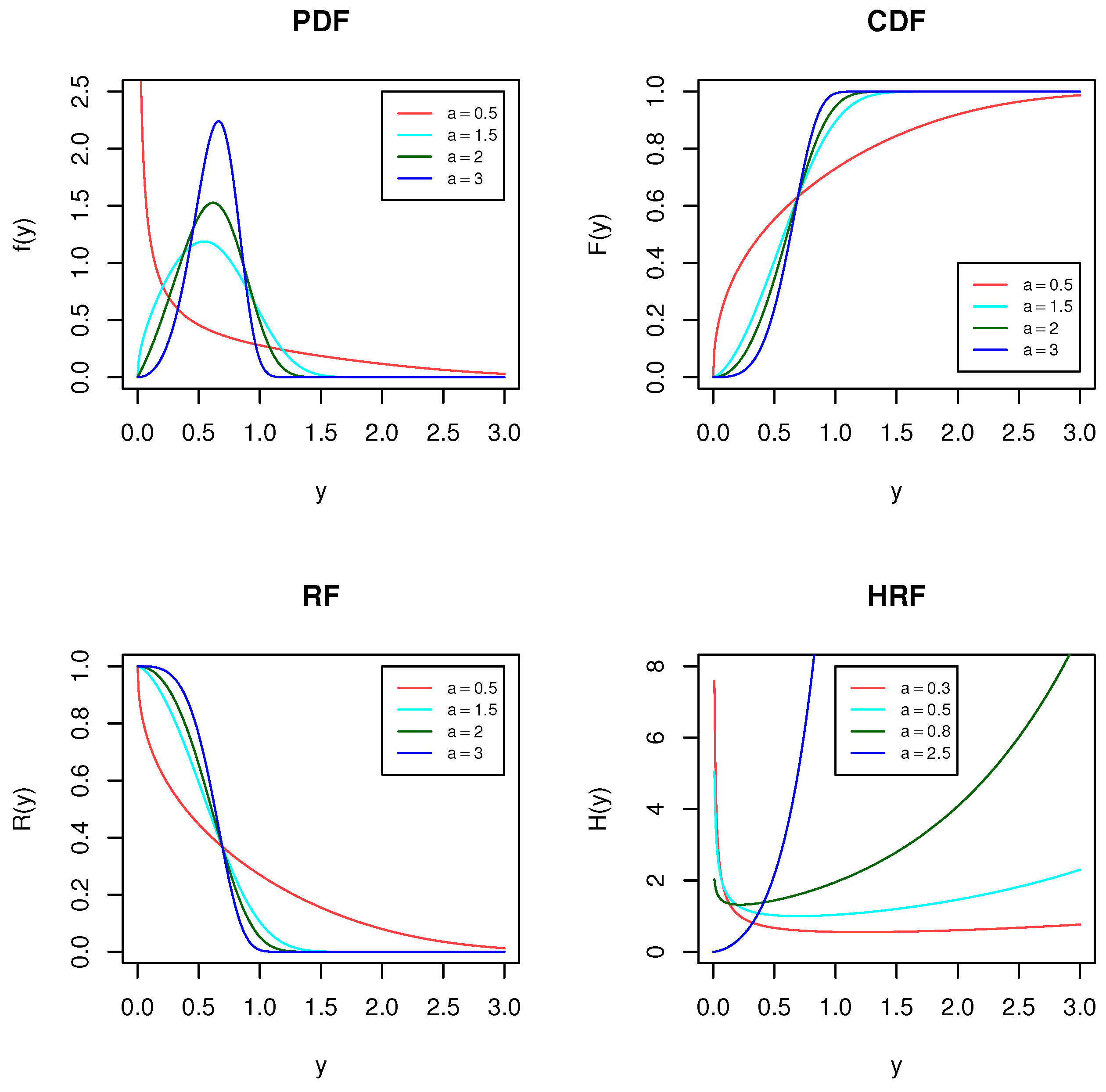
Figure 1 displays the different plots of the PDF, CDF, RF and HRF for some selected values of the shape parameter and assumes that the scale parameter is one in all the cases. Al-Babtain et al. [15] mentioned that the PDF of the MKE distribution can be symmetric or positive- or negative-skewed, depending on the shape parameter value. In addition, they proved that the HRF of the MKE distribution is increasing for $a\ge 1$ and bathtub-shaped for $a<1$. According to Al-Babtain et al. [15], the mean and median of the MKE distribution can be written, respectively, as

$$\mu =\sum _{m,j,k=0}^{\infty }\frac{a{(-1)}^{m+j}}{b{(1+m)}^{2}j!}\left(\begin{array}{c}k+a(j+1)\\ k\end{array}\right)\left(\begin{array}{c}k+a(j+1)-1\\ m\end{array}\right)$$

and

$$M=\frac{1}{b}log\left[1+{(log2)}^{1/a}\right].$$

Now, suppose that we have n units divided into two groups: the first group contains $n_1$ units randomly chosen from n test units at normal conditions, and the second group contains the remaining $n_2=n-n_1$ units, which are subjected to an accelerated condition. For group k, where $k=1,2$, the units are tested under the Type-II censoring scheme with prefixed sample size $(n_k,r_k)$, where $r_k\le n_k,k=1,2$, are the observed number of failures at normal use and accelerated conditions, respectively. Once the experiment ends, one has the observations $(Y_{k1},Y_{k2},\dots ,Y_{k{r}_k})$. The lifetime of an item tested at normal conditions follows the MKE distribution, with PDF, CDF, RF and HRF given by (1)–(4). The hazard rate of a tested unit at accelerated condition is given by $H_2\left(y\right)=c{H}_1\left(y\right)$, where $H_1\left(y\right)$ is given by (4) and c is an acceleration factor satisfying $c>1$. In this case, the HRF under the accelerated condition is given by

$$\begin{array}{ccc}\hfill H_2\left(y\right)& =& c{H}_1\left(y\right)\hfill \\ & =& abc{e}^{aby}{\left(1-e^{-by}\right)}^{a-1}.\hfill \end{array}$$

(5)

Using the relation $R_2\left(y\right)=exp\left(-{\int }_0^y{H}_2\left(x\right)dx\right)$, we can obtain the RF under the accelerated condition as follows:

$$R_2\left(y\right)=e^{-c{\left(e^{by}-1\right)}^a}.$$

(6)

The corresponding CDF and PDF are, respectively, given by

$$F_2\left(y\right)=1-e^{-c{\left(e^{by}-1\right)}^a}$$

(7)

and

$$f_2\left(y\right)=abc{e}^{aby-c{\left(e^{by}-1\right)}^a}{\left(1-e^{-by}\right)}^{a-1}.$$

(8)

It is of interest to mention here that one of the main advantages of the MKE distribution is that it contains only one scale and one shape parameter. Hence, this makes it a very flexible model when applied in the CSPALT because the number of parameters of the new model will be three, including the acceleration factor c. On the other hand, when using models with three parameters, such as the exponentiated Weibull distribution, the model parameters increase to four parameters (due to the acceleration factor). Therefore, the resulting model will be very complicated with many parameters, which makes it not a practical choice to many researchers and reliability engineers. Based on the previous argument, the likelihood function (without constant terms) based on the realizations of the two censored samples is given by

$$\begin{array}{c}\hfill L\left(\mathit{\theta }\right|y)=\prod _{k=1}^2\left\{\prod _{i=1}^{r_k}{f}_k\left(y_{ki}\right){[1-F_k\left(y_{k{r}_k}\right)]}^{n_k-r_k}\right\},\end{array}$$

(9)

where $\mathit{\theta }={(a,b,c)}^{\top }$. Cheng and Amin [20] proposed the MPS estimation method as an alternative to the ML estimation method, especially for the distributions with unknown scale and shifted threshold. They pointed out that the MPS and ML estimators have similar asymptotic sufficiency, consistency and efficiency properties. Ranneby [21] studied the mathematical properties of the MPS method as an approximation to the Kullback–Leibler information and observed that the MPS method gives unique and minimum variance unbiased estimators. In addition, Anatolyev and Kosenok [22] investigated the invariance properties of the MPS estimators (MPSEs) and showed that they have the same properties as the MLEs. The MPSEs are obtained by maximizing the product of the differences between the values of the CDF at adjacent ordered points. Ng et al. [23] extended the MPS method to estimate the parameters of a three-parameter Weibull distribution under progressively Type-II censored data. Following the same approach as Ng et al. [23], we can write the product of spacing to be maximized under the CSPALT for Type-II censored data as

$$\begin{array}{c}\hfill M\left(\mathit{\theta }\right|y)=\prod _{k=1}^2\left\{\prod _{i=1}^{r_k+1}[F_k\left(y_{ki}\right)-F_k\left(y_{ki-1}\right)]{[1-F_k\left(y_{k{r}_k}\right)]}^{n_k-r_k}\right\}.\end{array}$$

(10)

3. Maximum Likelihood Estimation

For $k=1,2$, let $Y_{k1}<Y_{k2}<\dots <Y_{k{r}_k}$ be two Type-II censored samples from two populations with CDFs and PDFs given by (2), (1), (7) and (8), respectively. In this case, we can write the log-likelihood function, denoted by $\ell \left(\mathit{\theta }\right|y)=logL(\mathit{\theta }\left|y\right)$, in the following form:

$$\begin{array}{ccc}\hfill \ell \left(\mathit{\theta }\right|y)& =& rlog\left(ab\right)+r_{2}log\left(c\right)+ab\sum _{k=1}^2\sum _{i=1}^{r_k}{y}_{ki}+(a-1)\sum _{k=1}^2\sum _{i=1}^{r_k}log\left({\psi }_{ki}\right)-\sum _{i=1}^{r_1}{\phi }_{1i}^a\hfill \\ & -& (n_1-r_1){\phi }_{1r_1}^a-c\left[\sum _{i=1}^{r_2}{\phi }_{2i}^a+(n_2-r_2){\phi }_{2r_2}^a\right],\hfill \end{array}$$

(11)

where $r=r_1+r_2,{\psi }_{ki}=1-e^{-b{y}_{ki}}$ and ${\phi }_{ki}=e^{b{y}_{ki}}-1$, $i=1,\dots ,r_k$. The maximum likelihood estimates (MLEs) of the parameters $a,b$ and c can be obtained by maximizing the objective function (11). This can be achieved by deriving (11) with respect to $a,b$ and c, equating them to zero, and then solving the system of nonlinear equations simultaneously. Here, the likelihood equations are as follows:

$$\begin{array}{ccc}\hfill \frac{\partial \ell \left(\mathit{\theta }\right|y)}{\partial a}& =& \frac{r}{a}+b\sum _{k=1}^2\sum _{i=1}^{r_k}{y}_{ki}+\sum _{k=1}^2\sum _{i=1}^{r_k}log\left({\psi }_{ki}\right)-\sum _{i=1}^{r_1}{\phi }_{1i}^{a}log\left({\phi }_{1i}\right)-(n_1-r_1){\phi }_{1r_1}^{a}log\left({\phi }_{1r_1}\right)\hfill \\ & -& c\left[\sum _{i=1}^{r_2}{\phi }_{2i}^{a}log\left({\phi }_{2i}\right)+(n_2-r_2){\phi }_{2r_2}^{a}log\left({\phi }_{2r_2}\right)\right]=0,\hfill \end{array}$$

(12)

$$\begin{array}{ccc}\hfill \frac{\partial \ell \left(\mathit{\theta }\right|y)}{\partial b}& =& \frac{r}{b}+a\sum _{k=1}^2\sum _{i=1}^{r_k}{y}_{ki}+(a-1)\sum _{k=1}^2\sum _{i=1}^{r_k}{y}_{ki}{\phi }_{ki}^{-1}-a\left[\sum _{i=1}^{r_1}{\eta }_{1i}+(n_1-r_1){\eta }_{1r_1}\right]\hfill \\ & -& ac\left[\sum _{i=1}^{r_2}{\eta }_{2i}+(n_2-r_2){\eta }_{2r_2}\right]=0\hfill \end{array}$$

(13)

and

$$\begin{array}{ccc}\hfill \frac{\partial \ell \left(\mathit{\theta }\right|y)}{\partial c}& =& \frac{r_2}{c}-\left[\sum _{i=1}^{r_2}{\phi }_{2i}^a+(n_2-r_2){\phi }_{2r_2}^a\right]=0,\hfill \end{array}$$

(14)

where ${\eta }_{ki}=y_{ki}{e}^{b{y}_{ki}}{\phi }_{ki}^{a-1},k=1,2$. From (14) and for fixed a and b, the MLE of the parameter c can be obtained as follows:

$$\begin{array}{ccc}\hfill \widehat{c}(a,b)& =& \frac{r_2}{{\sum }_{i=1}^{r_2}{\phi }_{2i}^a+(n_2-r_2){\phi }_{2r_2}^a}.\hfill \end{array}$$

(15)

Substituting $\widehat{c}(a,b)$, given by (15) in (12) and (13), the MLEs of a and b, denoted by $\widehat{a}$ and $\widehat{b}$, can be obtained by solving the following two nonlinear equations:

$$\begin{array}{c}\hfill \frac{r}{a}+b\sum _{k=1}^2\sum _{i=1}^{r_k}{y}_{ki}+\sum _{k=1}^2\sum _{i=1}^{r_k}log\left({\psi }_{ki}\right)-\sum _{i=1}^{r_1}{\phi }_{1i}^{a}log\left({\phi }_{1i}\right)-(n_1-r_1){\phi }_{1r_1}^{a}log\left({\phi }_{1r_1}\right)\\ \hfill -\frac{r_2\left[{\sum }_{i=1}^{r_2}{\phi }_{2i}^{a}log\left({\phi }_{2i}\right)+(n_2-r_2){\phi }_{2r_2}^{a}log\left({\phi }_{2r_2}\right)\right]}{{\sum }_{i=1}^{r_2}{\phi }_{2i}^a+(n_2-r_2){\phi }_{2r_2}^a}=0\end{array}$$

(16)

and

$$\begin{array}{c}\hfill \frac{r}{b}+a\sum _{k=1}^2\sum _{i=1}^{r_k}{y}_{ki}+(a-1)\sum _{k=1}^2\sum _{i=1}^{r_k}{y}_{ki}{\phi }_{ki}^{-1}-a\left[\sum _{i=1}^{r_1}{\eta }_{1i}+(n_1-r_1){\eta }_{1r_1}\right]\\ \hfill -\frac{a{r}_2\left[{\sum }_{i=1}^{r_2}{\eta }_{2i}+(n_2-r_2){\eta }_{2r_2}\right]}{{\sum }_{i=1}^{r_2}{\phi }_{2i}^a+(n_2-r_2){\phi }_{2r_2}^a}=0\end{array}$$

(17)

It is observed that, from (16) and (17), there are no closed forms for $\widehat{a}$ and $\widehat{b}$; therefore, any suitable numerical technique may be used to obtain these estimates. Upon obtaining $\widehat{a}$ and $\widehat{b}$, $\widehat{c}=\widehat{c}(\widehat{a},\widehat{b})$ can be obtained from (15) by replacing a and b with their corresponding estimates $\widehat{a}$ and $\widehat{b}$. Based on the asymptotic properties of the MLEs, we can construct the ACIs of the unknown parameters and the acceleration factor $\mathit{\theta }={(a,b,c)}^{\top }$. From large sample theory, it is known that the asymptotic distribution of the MLEs $\widehat{\mathit{\theta }}={(\widehat{a},\widehat{b},\widehat{c})}^{\top }$ is a trivariate normal distribution with mean $\mathit{\theta }$ and variance–covariance matrix ${\mathit{I}}^{-1}\left(\mathit{\theta }\right)$. Practically, ${\mathit{I}}^{-1}(\widehat{\mathit{\theta }})$ is used to estimate ${\mathit{I}}^{-1}\left(\mathit{\theta }\right)$, where $\mathit{I}(\widehat{\mathit{\theta }})$ is the observed information matrix and

$$\begin{array}{c}\hfill {\mathit{I}}^{-1}(\widehat{\mathit{\theta }})={\left(\begin{array}{ccc}-\frac{{\partial }^2\ell \left(\mathit{\theta }\right)}{\partial a^2}& -\frac{{\partial }^2\ell \left(\mathit{\theta }\right)}{\partial a\partial b}& -\frac{{\partial }^2\ell \left(\mathit{\theta }\right)}{\partial a\partial c}\\ -\frac{{\partial }^2\ell \left(\mathit{\theta }\right)}{\partial b\partial a}& -\frac{{\partial }^2\ell \left(\mathit{\theta }\right)}{\partial b^2}& -\frac{{\partial }^2\ell \left(\mathit{\theta }\right)}{\partial b\partial c}\\ -\frac{{\partial }^2\ell \left(\mathit{\theta }\right)}{\partial c\partial a}& -\frac{{\partial }^2\ell \left(\mathit{\theta }\right)}{\partial c\partial b}& -\frac{{\partial }^2\ell \left(\mathit{\theta }\right)}{\partial c^2}\end{array}\right)}_{(a,b,c)=(\widehat{a},\widehat{b},\widehat{c})}^{-1},\end{array}$$

(18)

where

$$\begin{array}{ccc}\hfill \frac{{\partial }^2\ell \left(\mathit{\theta }\right|y)}{\partial a^2}& =& -\frac{r}{a^2}-\sum _{i=1}^{r_1}{\phi }_{1i}^a{log}^2\left({\phi }_{1i}\right)-(n_1-r_1){\phi }_{1r_1}^a{log}^2\left({\phi }_{1r_1}\right)-c\sum _{i=1}^{r_2}{\phi }_{2i}^a{log}^2\left({\phi }_{2i}\right)\hfill \\ & -& c(n_2-r_2){\phi }_{2r_2}^a{log}^2\left({\phi }_{2r_2}\right),\hfill \end{array}$$

$$\begin{array}{ccc}\hfill \frac{{\partial }^2\ell \left(\mathit{\theta }\right|y)}{\partial b^2}& =& -\frac{r}{b^2}-(a-1)\sum _{k=1}^2\sum _{i=1}^{r_k}{y}_{ki}^2{e}^{b{y}_{ki}}{\phi }_{ki}^{-2}-a\sum _{i=1}^{r_1}{y}_{1i}{\eta }_{1i}[1+(a-1){\psi }_{1i}^{-1}]\hfill \\ & -& a(n_1-r_1)y_{1r_1}{\eta }_{1r_1}[1+(a-1){\psi }_{1r_1}^{-1}]-ac[\sum _{i=1}^{r_2}{y}_{2i}{\eta }_{2i}[1+(a-1){\psi }_{2i}^{-1}]\hfill \\ & +& (n_2-r_2)y_{2r_2}{\eta }_{2r_2}[1+(a-1){\psi }_{2r_2}^{-1}]],\hfill \end{array}$$

$$\begin{array}{ccc}\hfill \frac{{\partial }^2\ell \left(\mathit{\theta }\right|y)}{\partial c^2}& =& -\frac{r_2}{c^2},\hfill \end{array}$$

$$\begin{array}{ccc}\hfill \frac{{\partial }^2\ell \left(\mathit{\theta }\right|y)}{\partial a\partial b}& =& \sum _{k=1}^2\sum _{i=1}^{r_k}{y}_{ki}+\sum _{k=1}^2\sum _{i=1}^{r_k}{y}_{ki}{\phi }_{ki}^{-1}-\sum _{i=1}^{r_1}{\eta }_{1i}[1+alog\left({\phi }_{1i}\right)]-(n_1-r_1){\eta }_{1r_1}\hfill \\ & \times & [1+alog\left({\phi }_{1r_1}\right)]-c\left[\sum _{i=1}^{r_2}{\eta }_{2i}[1+alog\left({\phi }_{2i}\right)]+(n_2-r_2){\eta }_{2r_2}[1+alog\left({\phi }_{2r_2}\right)]\right],\hfill \end{array}$$

$$\begin{array}{c}\hfill \frac{{\partial }^2\ell \left(\mathit{\theta }\right|y)}{\partial a\partial c}=-\left[\sum _{i=1}^{r_2}{\phi }_{2i}^{a}log\left({\phi }_{2i}\right)+(n_2-r_2){\phi }_{2r_2}^{a}log\left({\phi }_{2r_2}\right)\right]\end{array}$$

and

$$\begin{array}{c}\hfill \frac{{\partial }^2\ell \left(\mathit{\theta }\right|y)}{\partial b\partial c}=-a\left[\sum _{i=1}^{r_2}{\eta }_{2i}+(n_2-r_2){\eta }_{2r_2}\right].\end{array}$$

Now, the $100(1-\alpha )\%$ ACIs of the unknown parameters $a,b$ and c can be obtained as follows:

$$\widehat{a}\pm z_{\alpha /2}\sqrt{\widehat{var}\left(\widehat{a}\right)},\widehat{b}\pm z_{\alpha /2}\sqrt{\widehat{var}\left(\widehat{b}\right)}\mathrm{and}\widehat{c}\pm z_{\alpha /2}\sqrt{\widehat{var}\left(\widehat{c}\right)}.$$

where $\widehat{var}(\widehat{a}),\widehat{var}(\widehat{b})$ and $\widehat{var}(\widehat{c})$ are the main diagonal elements of (18), respectively, and $z_{\alpha /2}$ is the upper $\alpha /2$th percentile point of the standard normal distribution.

Clearly, maximizing the objective function (11) with respect to $a,b$ and c to obtain the MLEs requires a numerical method using a statistical software such as R, which is an environment for statistical computing, see Reference [24]. Typically, researchers use Newton’s method (i.e., Newton–Raphson) to solve (12)–(14), with respect to the model parameters, to numerically determine the MLEs. Furthermore, they sometimes transform the model parameters using a log-transformation to avoid constraints, as indicated by MacDonald [25]. In R, the objective function (11) can be maximized using built-in functions of R, such as nlm() and optim(). However, since there is a constraint on the acceleration parameter c, namely, $c>1$, we could not apply any transformations on the model parameters to avoid constraints; thus, we considered the R built-in function nlminb(), which implements a constrained quasi-Newton method. For details about this approach, see Fox et al. [26].

4. Maximum Product of Spacing Estimation

In the maximum likelihood method approach, the values of the parameters are chosen to maximize the likelihood function. The MPSEs are computed instead by choosing the values of the parameters that maximize the product of the spaces between the values of the distribution function at adjacent ordered points. Anatolyev and Kosenok [22] stated that for small sample sizes, the MPSEs demonstrate efficient small sample behaviour when compared with the MLEs, which makes the MPS method even more appealing in reliability studies. For more details about the MPS estimation method, see Nassar et al. [27] and Basu et al. [28]. Using the same notation as the previous sections and from (2), (7) and (10), we can write the product of spacing to be maximized as follows:

$$\begin{array}{c}\hfill M\left(\mathit{\theta }\right|y)=\prod _{i=1}^{r_1+1}[e^{-{\phi }_{1i-1}^a}-e^{-{\phi }_{1i}^a}]\prod _{i=1}^{r_2+1}[e^{-c{\phi }_{2i-1}^a}-e^{-c{\phi }_{2i}^a}]e^{-\left[(n_1-r_1){\phi }_{1r_1}^a+c(n_2-r_2){\phi }_{2r_2}^a\right]}.\end{array}$$

(19)

Taking the natural logarithm of (19), say, $m\left(\mathit{\theta }\right|y)=logM(\mathit{\theta }\left|y\right)$, we have the following:

$$\begin{array}{ccc}\hfill m\left(\mathit{\theta }\right|y)& =& \sum _{i=1}^{r_1+1}log[e^{-{\phi }_{1i-1}^a}-e^{-{\phi }_{1i}^a}]+\sum _{i=1}^{r_2+1}log[e^{-c{\phi }_{2i-1}^a}-e^{-c{\phi }_{2i}^a}]-[(n_1-r_1){\phi }_{1r_1}^a\hfill \\ & +& c(n_2-r_2){\phi }_{2r_2}^a].\hfill \end{array}$$

(20)

The MPSEs are obtained by maximizing the objective function (20) with respect to the unknown parameters $a,b$ and c. These estimates can also be obtained by differentiating (20) with respect to $a,b$ and c, equating the results to zero, and then solving the three nonlinear equations simultaneously. The three normal equations of (20) are given by

$$\begin{array}{ccc}\hfill \frac{\partial m\left(\mathit{\theta }\right|y)}{\partial a}& =& \sum _{i=1}^{r_1+1}\frac{{\varphi }_{1i}-{\varphi }_{1i-1}}{e^{-{\phi }_{1i-1}^a}-e^{-{\phi }_{1i}^a}}+c\sum _{i=1}^{r_2+1}\frac{{\varphi }_{2i}-{\varphi }_{2i-1}}{e^{-c{\phi }_{2i-1}^a}-e^{-c{\phi }_{2i}^a}}-[(n_1-r_1){\phi }_{1r_1}^{a}log\left({\phi }_{1r_1}\right)\hfill \\ & +& c(n_2-r_2){\phi }_{2r_2}^{a}log\left({\phi }_{2r_2}\right)]=0,\hfill \end{array}$$

(21)

$$\begin{array}{ccc}\hfill \frac{\partial m\left(\mathit{\theta }\right|y)}{\partial b}& =& a\sum _{i=1}^{r_1+1}\frac{{\zeta }_{1i}-{\zeta }_{1i-1}}{e^{-{\phi }_{1i-1}^a}-e^{-{\phi }_{1i}^a}}+ac\sum _{i=1}^{r_2+1}\frac{{\zeta }_{2i}-{\zeta }_{2i-1}}{e^{-c{\phi }_{2i-1}^a}-e^{-c{\phi }_{2i}^a}}-a[(n_1-r_1){\eta }_{1r_1}\hfill \\ & +& c(n_2-r_2){\eta }_{2r_2}]=0\hfill \end{array}$$

(22)

and

$$\begin{array}{c}\hfill \frac{\partial m\left(\mathit{\theta }\right|y)}{\partial c}=\sum _{i=1}^{r_2+1}\frac{{\phi }_{2i}^a{e}^{-c{\phi }_{2i}^a}-{\phi }_{2i-1}^a{e}^{-c{\phi }_{2i-1}^a}}{e^{-c{\phi }_{2i-1}^a}-e^{-c{\phi }_{2i}^a}}-(n_2-r_2){\phi }_{2r_2}^a=0,\end{array}$$

(23)

where ${\varphi }_{1i}=e^{-{\phi }_{1i}^a}{\phi }_{1i}^{a}log\left({\phi }_{1i}\right)$, ${\varphi }_{2i}=e^{-c{\phi }_{2i}^a}{\phi }_{2i}^{a}log\left({\phi }_{2i}\right)$, ${\zeta }_{1i}={\eta }_{1i}{e}^{-{\phi }_{1i}^a}$ and ${\zeta }_{2i}={\eta }_{2i}{e}^{-c{\phi }_{2i}^a}$. It is noted that the MPSEs denoted by $\tilde{a},\tilde{b}$ and $\tilde{c}$ cannot be obtained in closed forms; therefore, numerical techniques can be used to solve Equations (21)–(23).

Using the same approach as the ML estimation method and from large sample theory, we constructed the ACI for the unknown parameters based on the MPSEs. The asymptotic distribution of the MPSEs $\tilde{\mathit{\theta }}={(\tilde{a},\tilde{b},\tilde{c})}^{\top }$ is a trivariate normal distribution with mean $\mathit{\theta }$ and variance–covariance matrix ${\mathit{I}}^{-1}\left(\mathit{\theta }\right)$. It is beneficial to remark here that several authors have elicited the asymptotic equivalence of the MPS method and ML estimation method; Cheng and Amin [20], Ghosh and Jammalamadaka [29] and Anatolyev and Kosenok [22] demonstrated that the MPS method exhibits asymptotic properties, like the ML method. One can also refer to Basu et al. [30,31]. In this case, we used ${\mathit{I}}^{-1}(\tilde{\mathit{\theta }})$ to estimate ${\mathit{I}}^{-1}\left(\mathit{\theta }\right)$ as follows:

$$\begin{array}{c}\hfill {\mathit{I}}^{-1}\left(\tilde{\mathit{\theta }}\right)={\left(\begin{array}{ccc}-\frac{{\partial }^2\ell \left(\mathit{\theta }\right)}{\partial a^2}& -\frac{{\partial }^2\ell \left(\mathit{\theta }\right)}{\partial a\partial b}& -\frac{{\partial }^2\ell \left(\mathit{\theta }\right)}{\partial a\partial c}\\ -\frac{{\partial }^2\ell \left(\mathit{\theta }\right)}{\partial b\partial a}& -\frac{{\partial }^2\ell \left(\mathit{\theta }\right)}{\partial b^2}& -\frac{{\partial }^2\ell \left(\mathit{\theta }\right)}{\partial b\partial c}\\ -\frac{{\partial }^2\ell \left(\mathit{\theta }\right)}{\partial c\partial a}& -\frac{{\partial }^2\ell \left(\mathit{\theta }\right)}{\partial c\partial b}& -\frac{{\partial }^2\ell \left(\mathit{\theta }\right)}{\partial c^2}\end{array}\right)}_{(a,b,c)=(\tilde{a},\tilde{b},\tilde{c})}^{-1},\end{array}$$

where

$$\begin{array}{ccc}\hfill \frac{{\partial }^{2}m\left(\mathit{\theta }\right|y)}{\partial a^2}& =& \sum _{i=1}^{r_1+1}\frac{{\varpi }_{1i}-{\varpi }_{1i-1}}{e^{-{\phi }_{1i-1}^a}-e^{-{\phi }_{1i}^a}}-\sum _{i=1}^{r_1+1}\frac{{({\varphi }_{1i}-{\varphi }_{1i-1})}^2}{{\left(e^{-{\phi }_{1i-1}^a}-e^{-{\phi }_{1i}^a}\right)}^2}+c\sum _{i=1}^{r_2+1}\frac{{\varpi }_{2i}-{\varpi }_{2i-1}}{e^{-{\phi }_{2i-1}^a}-e^{-{\phi }_{2i}^a}}\hfill \\ & -& c\sum _{i=1}^{r_2+1}\frac{{({\varphi }_{2i}-{\varphi }_{2i-1})}^2}{{\left(e^{-c{\phi }_{2i-1}^a}-e^{-c{\phi }_{2i}^a}\right)}^2}-(n_1-r_1){\phi }_{1r_1}^a{log}^2\left({\phi }_{1r_1}\right)-c(n_2-r_2){\phi }_{2r_2}^a{log}^2\left({\phi }_{2r_2}\right),\hfill \end{array}$$

$$\begin{array}{ccc}\hfill \frac{{\partial }^{2}m\left(\mathit{\theta }\right|y)}{\partial b^2}& =& a\sum _{i=1}^{r_1+1}\frac{{\varrho }_{1i}-{\varrho }_{1i-1}}{e^{-{\phi }_{1i-1}^a}-e^{-{\phi }_{1i}^a}}-a\sum _{i=1}^{r_1+1}\frac{{({\zeta }_{1i}-{\zeta }_{1i-1})}^2}{{\left(e^{-{\phi }_{1i-1}^a}-e^{-{\phi }_{1i}^a}\right)}^2}+ac\sum _{i=1}^{r_2+1}\frac{{\varrho }_{2i}-{\varrho }_{2i-1}}{{}^{-{\phi }_{2i-1}^a}-e^{-{\phi }_{2i}^a}}\hfill \\ & -& ac\sum _{i=1}^{r_2+1}\frac{{({\zeta }_{2i}-{\zeta }_{2i-1})}^2}{{\left(e^{-{\phi }_{2i-1}^a}-e^{-{\phi }_{2i}^a}\right)}^2}-a(n_1-r_1)y_{1_{r_1}}{\eta }_{1r_1}(1+(a-1){\psi }_{1r_1})\hfill \\ & -& ac(n_2-r_2)y_{2_{r_2}}{\eta }_{2r_2}(1+(a-1){\psi }_{2r_2}),\hfill \end{array}$$

$$\begin{array}{c}\hfill \frac{{\partial }^{2}m\left(\mathit{\theta }\right|y)}{\partial c^2}=\sum _{i=1}^{r_2+1}\frac{{\phi }_{2i-1}^{2a}{e}^{-c{\phi }_{2i-1}^a}-{\phi }_{2i}^{2a}{e}^{-c{\phi }_{2i}^a}}{e^{-c{\phi }_{2i-1}^a}-e^{-c{\phi }_{2i}^a}}-\sum _{i=1}^{r_2+1}\frac{{\left({\phi }_{2i}^a{e}^{-c{\phi }_{2i}^a}-{\phi }_{2i-1}^a{e}^{-c{\phi }_{2i-1}^a}\right)}^2}{{\left(e^{-c{\phi }_{2i-1}^a}-e^{-c{\phi }_{2i}^a}\right)}^2},\end{array}$$

$$\begin{array}{ccc}\hfill \frac{{\partial }^{2}m\left(\mathit{\theta }\right|y)}{\partial a\partial b}& =& \sum _{i=1}^{r_1+1}\frac{{\tau }_{1i}-{\tau }_{1i-1}}{e^{-{\phi }_{1i-1}^a}-e^{-{\phi }_{1i}^a}}-\sum _{i=1}^{r_1+1}\frac{({\varphi }_{1i}-{\varphi }_{1i-1})({\zeta }_{1i}-{\zeta }_{1i-1})}{{\left(e^{-{\phi }_{1i-1}^a}-e^{-{\phi }_{1i}^a}\right)}^2}+c\sum _{i=1}^{r_2+1}\frac{{\tau }_{2i}-{\tau }_{2i-1}}{e^{-c{\phi }_{2i-1}^a}-e^{c-{\phi }_{2i}^a}}\hfill \\ & -& c\sum _{i=1}^{r_2+1}\frac{({\varphi }_{2i}-{\varphi }_{2i-1})({\zeta }_{2i}-{\zeta }_{2i-1})}{{\left(e^{-c{\phi }_{2i-1}^a}-e^{-c{\phi }_{2i}^a}\right)}^2}-a(n_1-r_1){\eta }_{1r_1}log\left({\phi }_{1r_1}\right)\hfill \\ & -& ac(n_2-r_2){\eta }_{2r_2}log\left({\phi }_{2r_2}\right),\hfill \end{array}$$

$$\begin{array}{ccc}\hfill \frac{{\partial }^{2}m\left(\mathit{\theta }\right|y)}{\partial a\partial c}& =& c\sum _{i=1}^{r_2+1}\frac{{\varphi }_{2i-1}{\phi }_{2i-1}^a-{\varphi }_{2i}{\phi }_{2i}^a}{e^{-c{\phi }_{2i-1}^a}-e^{-c{\phi }_{2i}^a}}-c\sum _{i=1}^{r_2+1}\frac{({\varphi }_{2i}-{\varphi }_{2i-1})({\phi }_{2i}^a{e}^{-c{\phi }_{2i}^a}-{\phi }_{2i-1}^a{e}^{-c{\phi }_{2i-1}^a})}{{\left(e^{-c{\phi }_{2i-1}^a}-e^{-c{\phi }_{2i}^a}\right)}^2}\hfill \\ & +& \sum _{i=1}^{r_2+1}\frac{{\varphi }_{2i}-{\varphi }_{2i-1}}{e^{-c{\phi }_{2i-1}^a}-e^{-c{\phi }_{2i}^a}}-(n_2-r_2){\phi }_{2r_2}^{a}log\left({\phi }_{2r_2}\right)\hfill \end{array}$$

and

$$\begin{array}{ccc}\hfill \frac{{\partial }^{2}m\left(\mathit{\theta }\right|y)}{\partial b\partial c}& =& ac\sum _{i=1}^{r_2+1}\frac{{\zeta }_{2i-1}{\phi }_{2i-1}^{-a}-{\zeta }_{2i}{\phi }_{2i}^{-a}}{e^{-c{\phi }_{2i-1}^a}-e^{-c{\phi }_{2i}^a}}-ac\sum _{i=1}^{r_2+1}\frac{({\zeta }_{2i}-{\zeta }_{2i-1})({\phi }_{2i}^a{e}^{-c{\phi }_{2i}^a}-{\phi }_{2i-1}^a{e}^{-c{\phi }_{2i-1}^a})}{e^{-c{\phi }_{2i-1}^a}-e^{-c{\phi }_{2i}^a}}\hfill \\ & +& a\sum _{i=1}^{r_2+1}\frac{{\zeta }_{2i}-{\zeta }_{2i-1}}{e^{-c{\phi }_{2i-1}^a}-e^{-c{\phi }_{2i}^a}}-a(n_2-r_2){\eta }_{2r_2},\hfill \end{array}$$

where ${\varpi }_{1i}={\varphi }_{1i}log\left({\phi }_{1i}\right)(1-{\phi }_{1i}^a),{\varpi }_{2i}={\varphi }_{2i}log\left({\phi }_{2i}\right)(1-c{\phi }_{2i}^a)$, ${\varrho }_{1i}=y_{1i}{\zeta }_{1i}[1+e^{b{y}_{1i}}{\phi }_{1i}^{-1}(a(1-{\phi }_{1i}^a)-1)]$, ${\varrho }_{2i}=y_{2i}{\zeta }_{2i}[1+e^{b{y}_{2i}}{\phi }_{2i}^{-1}(a(1-c{\phi }_{2i}^a)-1)]$, ${\tau }_{1i}=alog\left({\phi }_{1i}\right){\eta }_{1i}{e}^{-{\phi }_{1i}^a}(1-{\phi }_{1i}^a)$ and ${\tau }_{2i}=alog\left({\phi }_{2i}\right){\eta }_{2i}{e}^{-c{\phi }_{2i}^a}(1-c{\phi }_{2i}^a)$. Now, the $100(1-\alpha )\%$ ACIs of the unknown parameters $a,b$ and c based on the MPSEs can be obtained:

$$\tilde{a}\pm z_{\alpha /2}\sqrt{\widehat{var}\left(\tilde{a}\right)},\tilde{b}\pm z_{\alpha /2}\sqrt{\widehat{var}\left(\tilde{b}\right)}\mathrm{and}\tilde{c}\pm z_{\alpha /2}\sqrt{\widehat{var}\left(\tilde{c}\right)}.$$

where $\widehat{var}\left(\tilde{a}\right),\widehat{var}\left(\tilde{b}\right)$ and $\widehat{var}\left(\tilde{c}\right)$ are the estimated variances.

Similar to MLEs, maximizing the objective function (20) with respect to $a,b$ and c to obtain MPSEs also requires a numerical method using R. We considered the same R built-in function nlminb() that implements a constraint quasi-Newton method to obtain the MPSEs.

5. Bootstrap Confidence Intervals

In this subsection, we consider using two parametric bootstrap confidence intervals. The first is the percentile bootstrap confidence interval (PBCI) method based on the idea of Efron [32]. The second is the studentized bootstrap confidence interval (SBCI) method proposed by Hall [33]. It is to be mentioned here that we obtained these two bootstrap confidence intervals based on MLEs and MPSEs. To compute these confidence intervals, we used the following steps.

(A) PBCIs

(1)

Based on the original data $Y_{k1}<Y_{k2}<\dots <Y_{k{r}_k},k=1,2$, obtain the MLEs and MPSEs.

(2)

Use the MLEs obtained in (1) to generate Type-II censored samples.

(3)

Redo step (2) using the MPSEs.

(4)

Use the generated bootstrap samples in (2) to obtain bootstrap estimates, denoted by ${\widehat{a}}^{*},{\widehat{b}}^{*}$ and ${\widehat{c}}^{*}$.

(5)

Use the generated bootstrap samples in (3) to obtain bootstrap estimates, denoted by ${\tilde{a}}^{*},{\tilde{b}}^{*}$ and ${\tilde{c}}^{*}$.

(6)

Repeat steps 2 and 4 B times to compute (${\widehat{a}}_1^{*},\dots ,{\widehat{a}}_B^{*}$), (${\widehat{b}}_1^{*},\dots ,{\widehat{b}}_B^{*}$) and (${\widehat{c}}_1^{*},\dots ,{\widehat{c}}_B^{*}$).

(7)

Repeat steps 3 and 5 B times to compute (${\tilde{a}}_1^{*},\dots ,{\tilde{a}}_B^{*}$), (${\tilde{b}}_1^{*},\dots ,{\tilde{b}}_B^{*}$) and (${\tilde{c}}_1^{*},\dots ,{\tilde{c}}_B^{*}$).

(8)

Arrange the estimates in (6) in ascending order to obtain (${\widehat{a}}_{\left[1\right]}^{*},\dots ,{\widehat{a}}_{\left[B\right]}^{*}$), (${\widehat{b}}_{\left[1\right]}^{*},\dots ,{\widehat{b}}_{\left[B\right]}^{*}$) and (${\widehat{c}}_{\left[1\right]}^{*},\dots ,{\widehat{c}}_{\left[B\right]}^{*}$).

(9)

Based on the MLEs, the two-sided $100(1-\alpha )\%$ PBCIs are given by

$$\left[{\widehat{a}}_{[B\alpha /2]}^{*},{\widehat{a}}_{\left[B\right(1-\alpha /2\left)\right]}^{*}\right],\left[{\widehat{b}}_{[B\alpha /2]}^{*},{\widehat{b}}_{\left[B\right(1-\alpha /2\left)\right]}^{*}\right] \mathrm{and} \left[{\widehat{c}}_{[B\alpha /2]}^{*},{\widehat{c}}_{\left[B\right(1-\alpha /2\left)\right]}^{*}\right].$$

(10)

Arrange the estimates in (7) in ascending order to obtain (${\tilde{a}}_{\left[1\right]}^{*},\dots ,{\widetilde{*}}_{\left[B\right]}^{*}$), (${\tilde{b}}_{\left[1\right]}^{*},\dots ,{\tilde{b}}_{\left[B\right]}^{*}$) and (${\tilde{c}}_{\left[1\right]}^{*},\dots ,{\tilde{c}}_{\left[B\right]}^{*}$).

(11)

Based on the MPSEs, the two-sided $100(1-\alpha )\%$ PBCIs are given by

$$\left[{\tilde{a}}_{[B\alpha /2]}^{*},{\tilde{a}}_{\left[B\right(1-\alpha /2\left)\right]}^{*}\right],\left[{\tilde{b}}_{[B\alpha /2]}^{*},{\tilde{b}}_{\left[B\right(1-\alpha /2\left)\right]}^{*}\right] \mathrm{and} \left[{\tilde{c}}_{[B\alpha /2]}^{*},{\tilde{c}}_{\left[B\right(1-\alpha /2\left)\right]}^{*}\right].$$

(B) SBCIs

(1–5)

Same as in PBCIs.

(6)

Obtain the statistics $T^{*a}=\frac{{\widehat{a}}^{*}-\widehat{a}}{\sqrt{\widehat{var}\left({\widehat{a}}^{*}\right)}}$, $T^{*b}=\frac{{\widehat{b}}^{*}-\widehat{b}}{\sqrt{\widehat{var}\left({\widehat{b}}^{*}\right)}}$ and $T^{*c}=\frac{{\widehat{c}}^{*}-\widehat{c}}{\sqrt{\widehat{var}\left({\widehat{c}}^{*}\right)}}$.

(7)

Obtain the statistics $T^{\star a}=\frac{{\tilde{a}}^{*}-\tilde{a}}{\sqrt{\widehat{var}\left({\tilde{a}}^{*}\right)}}$, $T^{\star b}=\frac{{\tilde{b}}^{*}-\tilde{b}}{\sqrt{\widehat{var}\left({\tilde{b}}^{*}\right)}}$ and $T^{\star c}=\frac{{\tilde{c}}^{*}-\tilde{c}}{\sqrt{\widehat{var}\left({\tilde{c}}^{*}\right)}}$.

(8)

Repeat steps 2, 4 and 6 B times to obtain ($T_1^{*a},\dots ,T_B^{*a}$), ($T_1^{*b},\dots ,T_B^{*b}$) and ($T_1^{*c},\dots ,T_B^{*c}$).

(9)

Arrange the $T^{*}$-statistics in ascending order to obtain ($T_{\left[1\right]}^{*a},\dots ,T_{\left[B\right]}^{*a}$), ($T_{\left[1\right]}^{*b},\dots ,T_{\left[B\right]}^{*b}$) and ($T_{\left[1\right]}^{*c},\dots ,T_{\left[B\right]}^{*c}$).

(10)

Repeat steps 3, 5 and 7 B times to obtain ($T_1^{\star a},\dots ,T_B^{\star a}$), ($T_1^{\star b},\dots ,T_B^{\star b}$) and ($T_1^{\star c},\dots ,T_B^{\star c}$).

(11)

Arrange the $T^{\star }$-statistics in ascending order to obtain ($T_{\left[1\right]}^{\star a},\dots ,T_{\left[B\right]}^{\star a}$), ($T_{\left[1\right]}^{\star b},\dots ,T_{\left[B\right]}^{\star b}$) and ($T_{\left[1\right]}^{\star c},\dots ,T_{\left[B\right]}^{\star c}$).

(12)

Based on the MLEs, the two-sided $100(1-\alpha )$ SBCIs are given by

$$\begin{array}{ccc}& & \left[\widehat{a}+T_{[B\alpha /2]}^{*a}\sqrt{\widehat{var}\left(\widehat{a}\right)},\widehat{a}+T_{\left[B\right(1-\alpha /2\left)\right]}^{*a}\sqrt{\widehat{var}\left(\widehat{a}\right)}\right],\hfill \\ & & \left[\widehat{b}+T_{[B\alpha /2]}^{*b}\sqrt{\widehat{var}\left(\widehat{b}\right)},\widehat{b}+T_{\left[B\right(1-\alpha /2\left)\right]}^{*b}\sqrt{\widehat{var}\left(\widehat{b}\right)}\right]\hfill \\ \hfill \mathrm{and}\\ & & \left[\widehat{c}+T_{[B\alpha /2]}^{*c}\sqrt{\widehat{var}\left(\widehat{c}\right)},\widehat{c}+T_{\left[B\right(1-\alpha /2\left)\right]}^{*c}\sqrt{\widehat{var}\left(\widehat{c}\right)}\right].\hfill \end{array}$$

(13)

Based on the MPSEs, the two-sided $100(1-\alpha )$ SBCIs are given by

$$\begin{array}{ccc}& & \left[\tilde{a}+T_{[B\alpha /2]}^{\star a}\sqrt{\widehat{var}\left(\tilde{a}\right)},\tilde{a}+T_{\left[B\right(1-\alpha /2\left)\right]}^{\star a}\sqrt{\widehat{var}\left(\tilde{a}\right)}\right],\hfill \\ & & \left[\tilde{b}+T_{[B\alpha /2]}^{\star b}\sqrt{\widehat{var}\left(\tilde{b}\right)},\tilde{b}+T_{\left[B\right(1-\alpha /2\left)\right]}^{\star b}\sqrt{\widehat{var}\left(\tilde{b}\right)}\right]\hfill \\ \hfill \mathrm{and}\\ & & \left[\tilde{c}+T_{[B\alpha /2]}^{\star c}\sqrt{\widehat{var}\left(\tilde{c}\right)},\tilde{c}+T_{\left[B\right(1-\alpha /2\left)\right]}^{\star c}\sqrt{\widehat{var}\left(\tilde{c}\right)}\right].\hfill \end{array}$$

6. Simulation Studies

In this section, the outcomes of the analysis of a simulated data set from the described model are first presented in an illustrative example; afterwards, results from a Monte Carlo simulation study are reported. All results in this section are associated with proper discussions. It is important to mention that obtaining explicit estimators from the systems of nonlinear equations, which were mentioned in the previous sections, is typically not possible. In our case, we had three parameters; thus, we were dealing with three complicated nonlinear equations. That is why we obtained the desired estimators numerically.

Moreover, since we derived first- and second-order derivatives for the objective functions, we considered Newton’s method to find MLEs and MPSEs. Convergence problems might occur in any optimization process if the initial values are not chosen carefully by the researchers; we randomly generated initial values close to the actual model parameters. To optimize the objective function, we considered Newton’s method, which is known for its fast quadratic convergence. We do not provide details about this method for the sake of brevity.

6.1. Illustrative Example

Here, the MLEs and the MPSEs were determined numerically from a data set simulated from a CSPALT with $n_1=n_2=10$ and $a=1,b=1$ and $c=2$. The observations are reported in

Table 1. Simulated CSPALT data with complete information from which the Type-II censored data were obtained.

Normal Use Condition:

0.04557, 0.29199, 0.42258, 0.47619, 0.56019, 0.58873, 0.93712, 1.14605, 1.17233, 1.34057

Accelerated Stress Condition:

0.02305, 0.15661, 0.23345, 0.26618, 0.31882, 0.33708, 0.57454, 0.72893, 0.74894, 0.87988

.

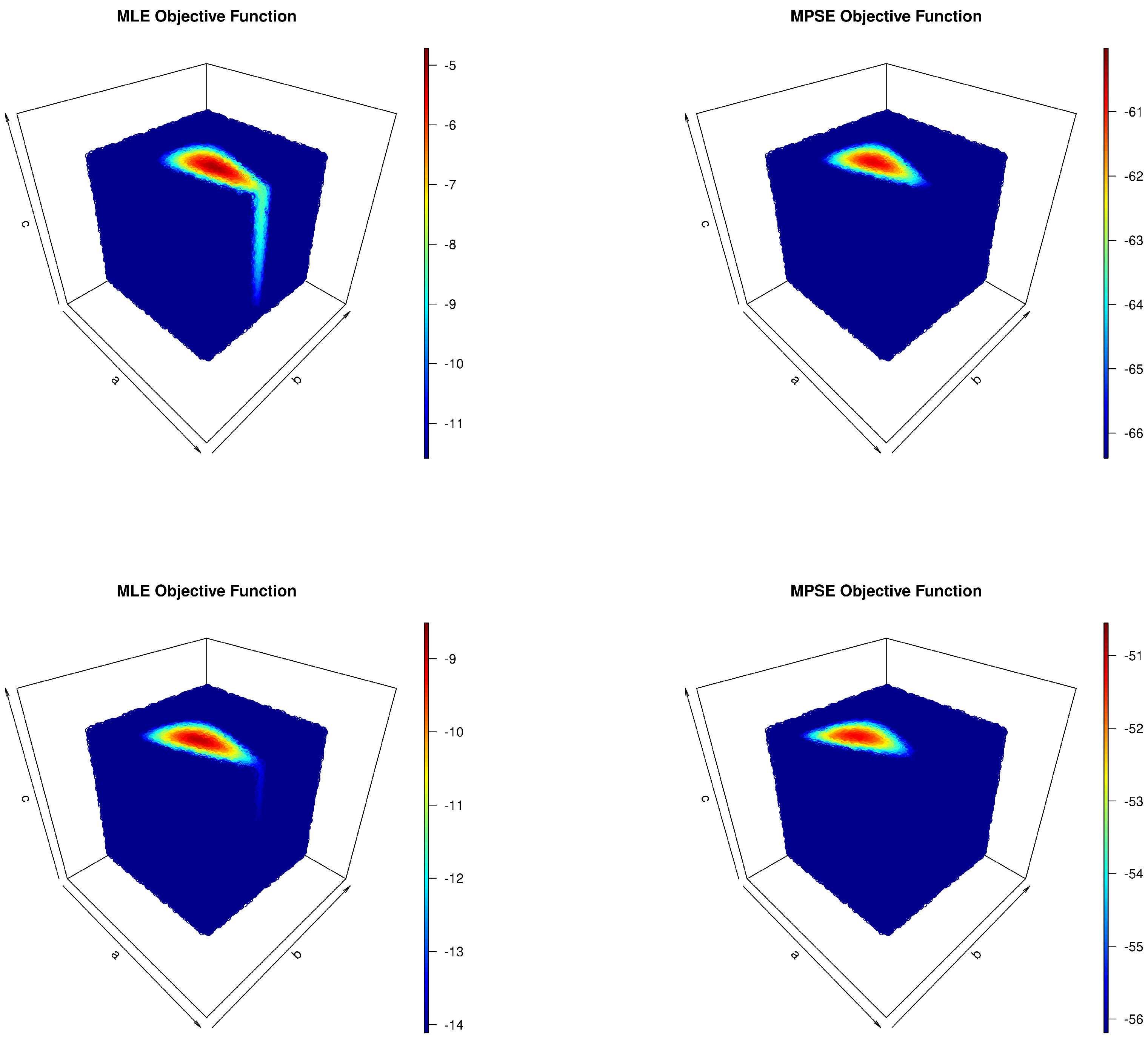
Type-II censored data were derived from the data in Table 1 under the assumption that $r_1=r_2=8$. Before proceeding to the calculation of the MLEs and the MPSEs for the model parameters, one must check their existence and uniqueness and whether the data are complete or not. Although proving these conditions is extremely important mathematically, it is beyond this study’s scope. However, one could still prove such requirements by using graphical means. In fact, by using extensive Monte Carlo simulations, a four-dimensional (4D) plot for the profiles of the objective functions of MLEs and MPSEs was established, as shown in Figure 2, in the case of complete and censored data. The 4D charts clearly show regions, namely, the dark-red spots, in which global maxima exist and are unique for the objective functions. In addition, censoring caused the regions to slightly change their forms and shift from their original places when the data were uncensored. The starting values for the model parameters were obtained from the Monte Carlo simulations to optimize the objective function and are reported in

Table 2. Starting (initial) values from the objective functions, based on Table 1.

Case	${\mathit{a}}_{\mathbf{0}}$	${\mathit{b}}_{\mathbf{0}}$	${\mathit{c}}_{\mathbf{0}}$
MLEs–Complete	1.2454	0.8690	2.2633
MPSEs–Complete	0.9775	0.8690	1.8312
MLEs–Censoring	1.1003	0.8020	2.0485
MPSEs–Censoring	0.8382	0.7628	1.6506

. The reason for having different initial values is that we were dealing with two different objective functions under two different data settings. The initial values that maximize the log-likelihood function might not necessarily maximize the maximum product of spacing objective function. Nevertheless, the initial values that maximize the log-likelihood function can still obtain the MPSEs. By using these initial values in Table 2, the estimates of the model parameters and their asymptotic variances evaluated at these estimates are given in

Table 3. Estimates and their asymptotic properties, based on Table 1.

Case	a	b	c	$\mathbf{Var}(\widehat{\mathit{a}})$	$\mathbf{Var}(\widehat{\mathit{b}})$	$\mathbf{Var}(\widehat{\mathit{c}})$
MLEs–Complete	1.25035	0.87498	2.21597	0.06037	0.02388	1.03754
MPSEs–Complete	0.97684	0.86682	1.82586	0.04423	0.03754	0.69076
MLEs–Censoring	1.09137	0.80231	2.02881	0.05727	0.03321	1.07325
MPSEs–Censoring	0.83742	0.75583	1.69290	0.04061	0.05133	0.73330

. From this table, one can readily conclude that MLEs provided estimates close to the true values of the model parameters compared to the MPSEs when the data were complete or censored and that censoring increased the values of the approximated asymptotic variations of the estimates. Further comparisons are conducted in the upcoming subsection to investigate the performance of the MLEs and MPSEs.

6.2. Simulation Method and Outcomes

This subsection reports the results of a simulation study conducted based on Monte Carlo methods to examine the efficiency of the considered estimators numerically. The performance of the MLEs and MPSEs was assessed in terms of simulated biases and simulated root-mean-square errors (RMSEs). In this simulation study, the model parameters were considered to be $a=0.5,2$, $b=1$ and $c=1.5,2.5$. Furthermore, it was assumed that $n_1=n_2$ and $r_1=r_2$ for the sake of concision; moreover, the following Type-II censoring settings were considered in both normal use and accelerated stress stages:

• $n_1=n_2=20$ and $r_1=r_2=12$.
• $n_1=n_2=20$ and $r_1=r_2=16$.
• $n_1=n_2=40$ and $r_1=r_2=24$.
• $n_1=n_2=40$ and $r_1=r_2=32$.
• $n_1=n_2=60$ and $r_1=r_2=36$.
• $n_1=n_2=60$ and $r_1=r_2=48$.
• $n_1=n_2=80$ and $r_1=r_2=48$.
• $n_1=n_2=80$ and $r_1=r_2=64$.
• $n_1=n_2=100$ and $r_1=r_2=60$.
• $n_1=n_2=100$ and $r_1=r_2=80$.

By maximizing the objective functions (11) and (20) with respect to $a,b$ and c using R, we obtained the MLEs and the MPSEs for the model parameters, as mentioned in the previous sections. Due to the fact that there is no information about the range of the estimates in practice, the starting values of the model parameters were randomly obtained around their true values, assuming independent uniform distributions. From a practical perspective, one should alternatively consider computational ranges for the model parameters and perform profiling on the objective functions to acquire the corresponding starting values. For more details about best practice optimization approaches in R, see Nash [34].

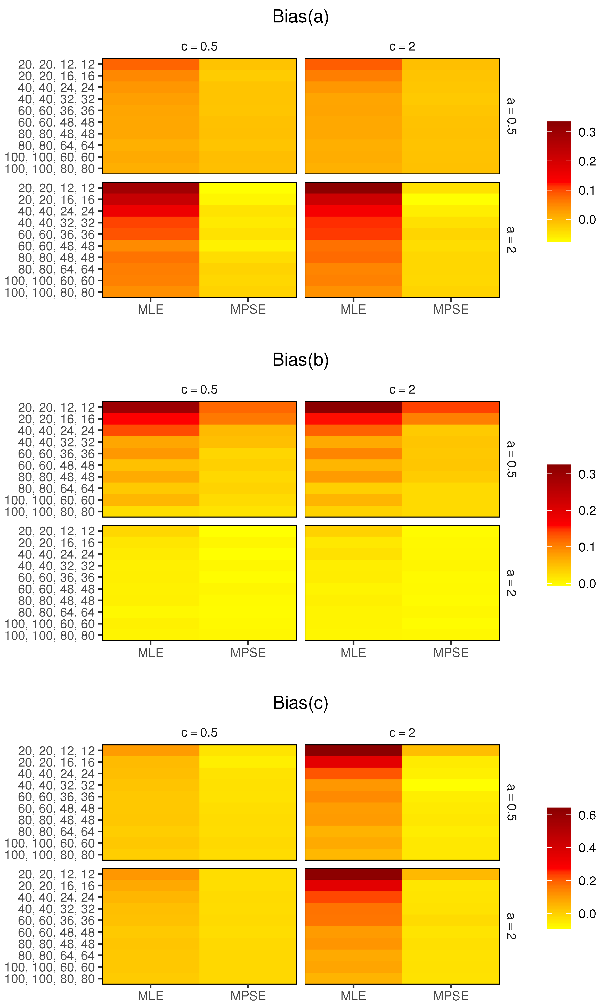
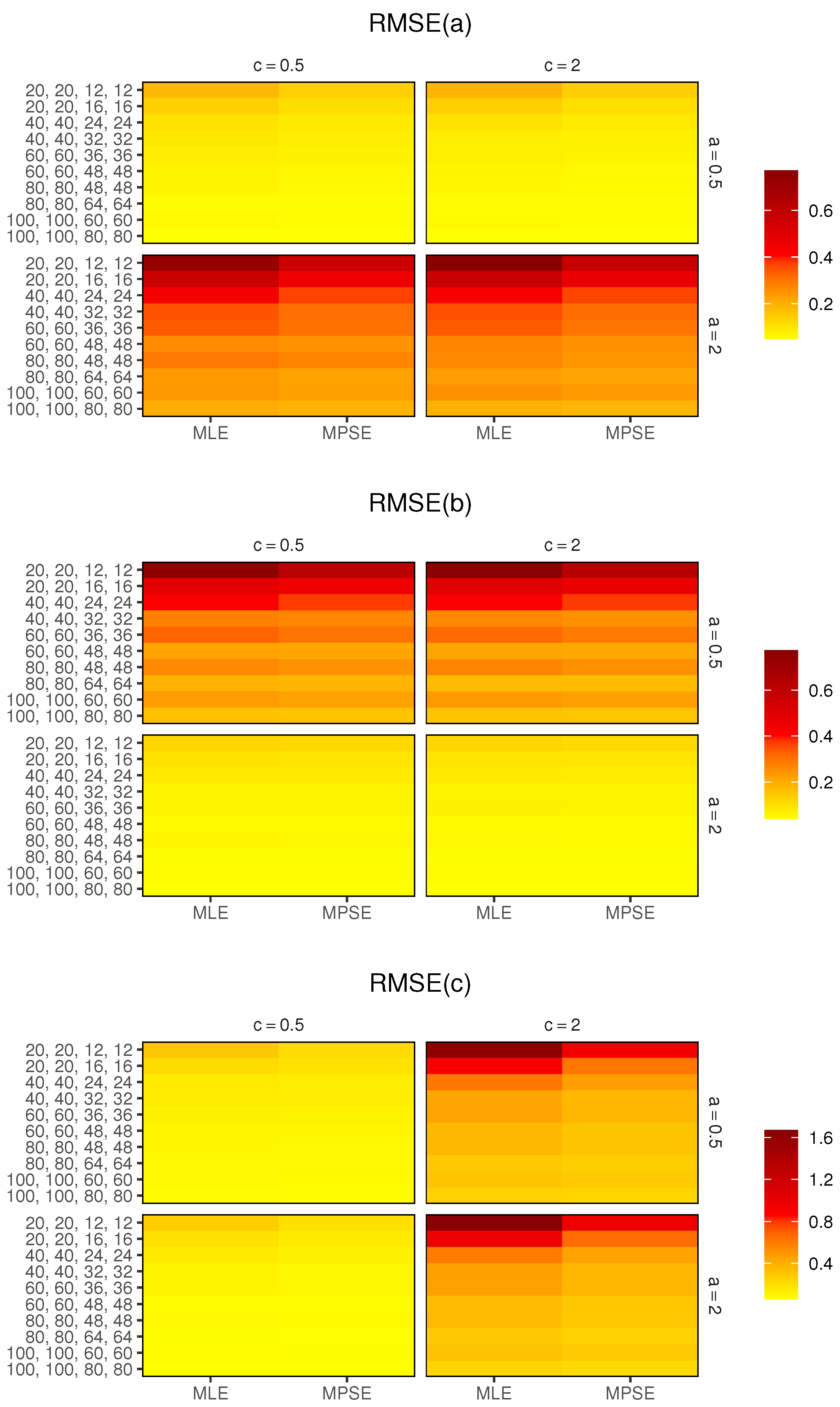
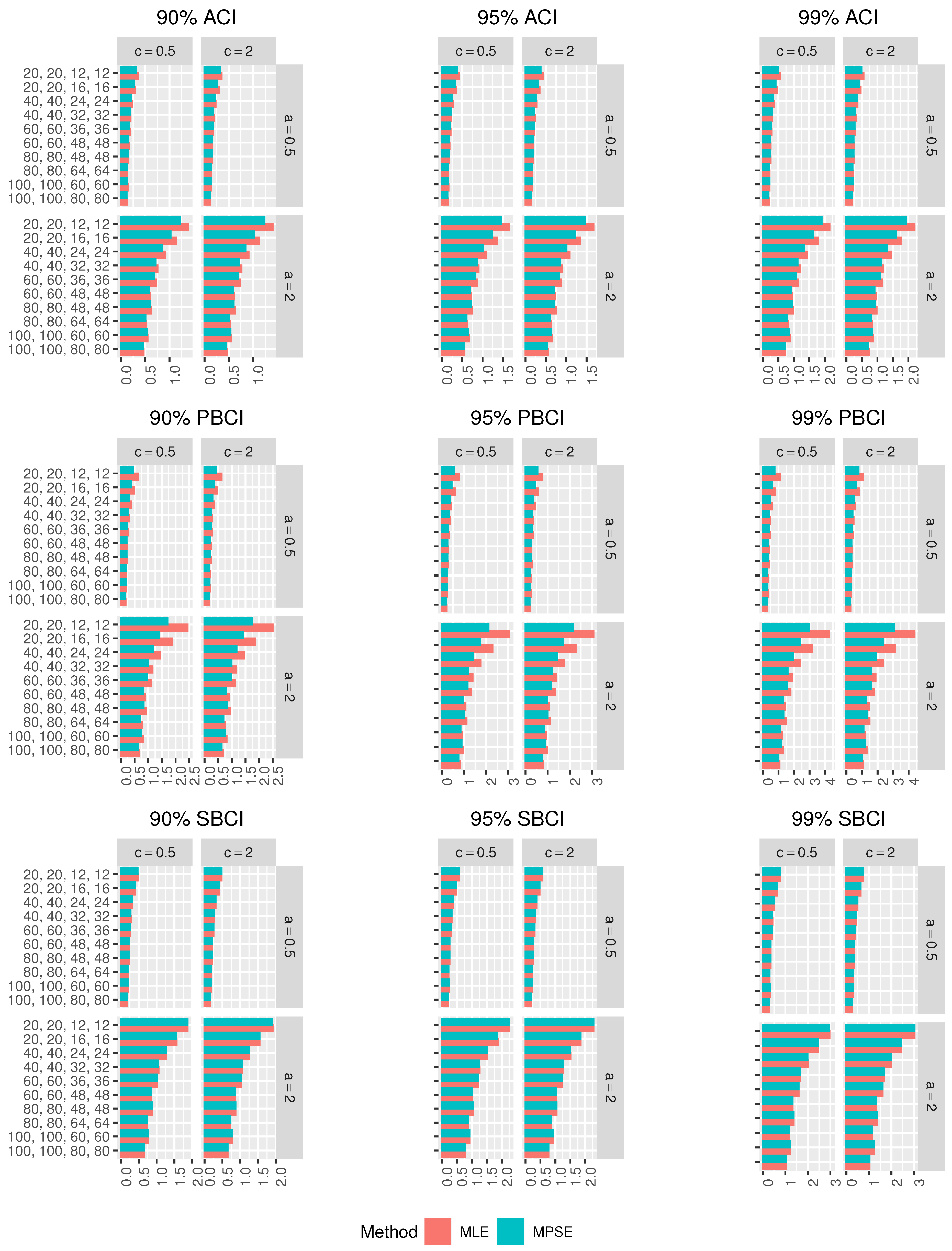
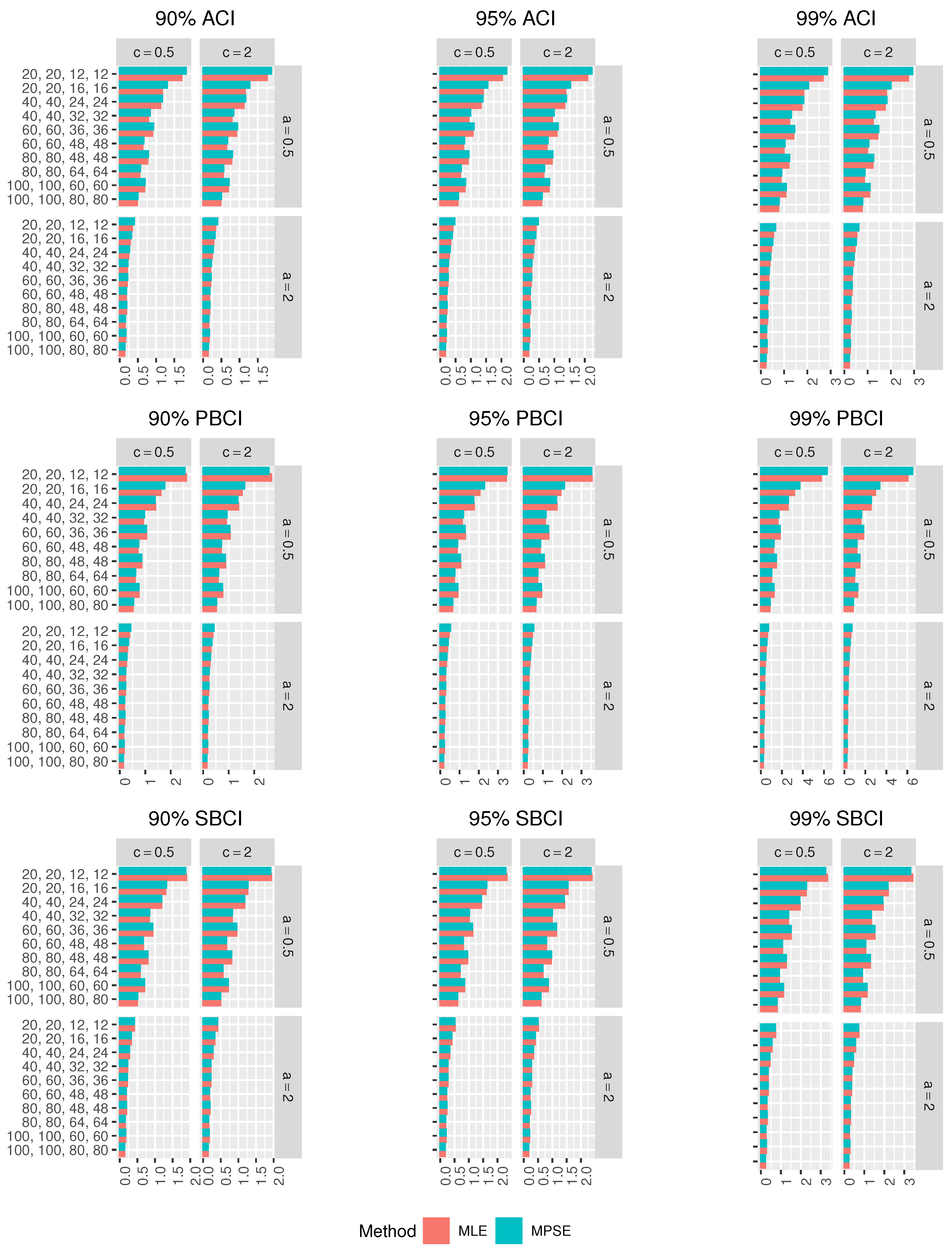
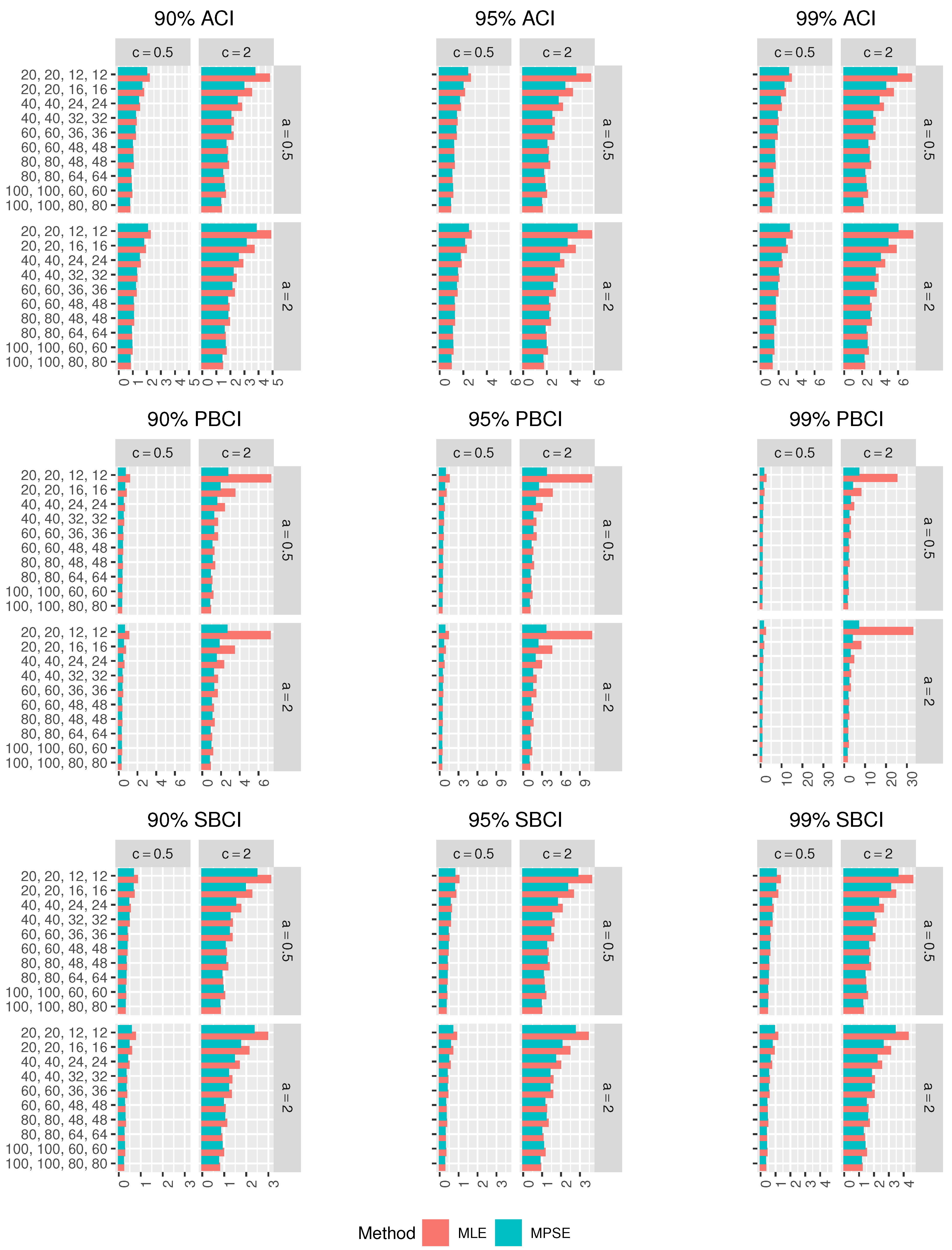
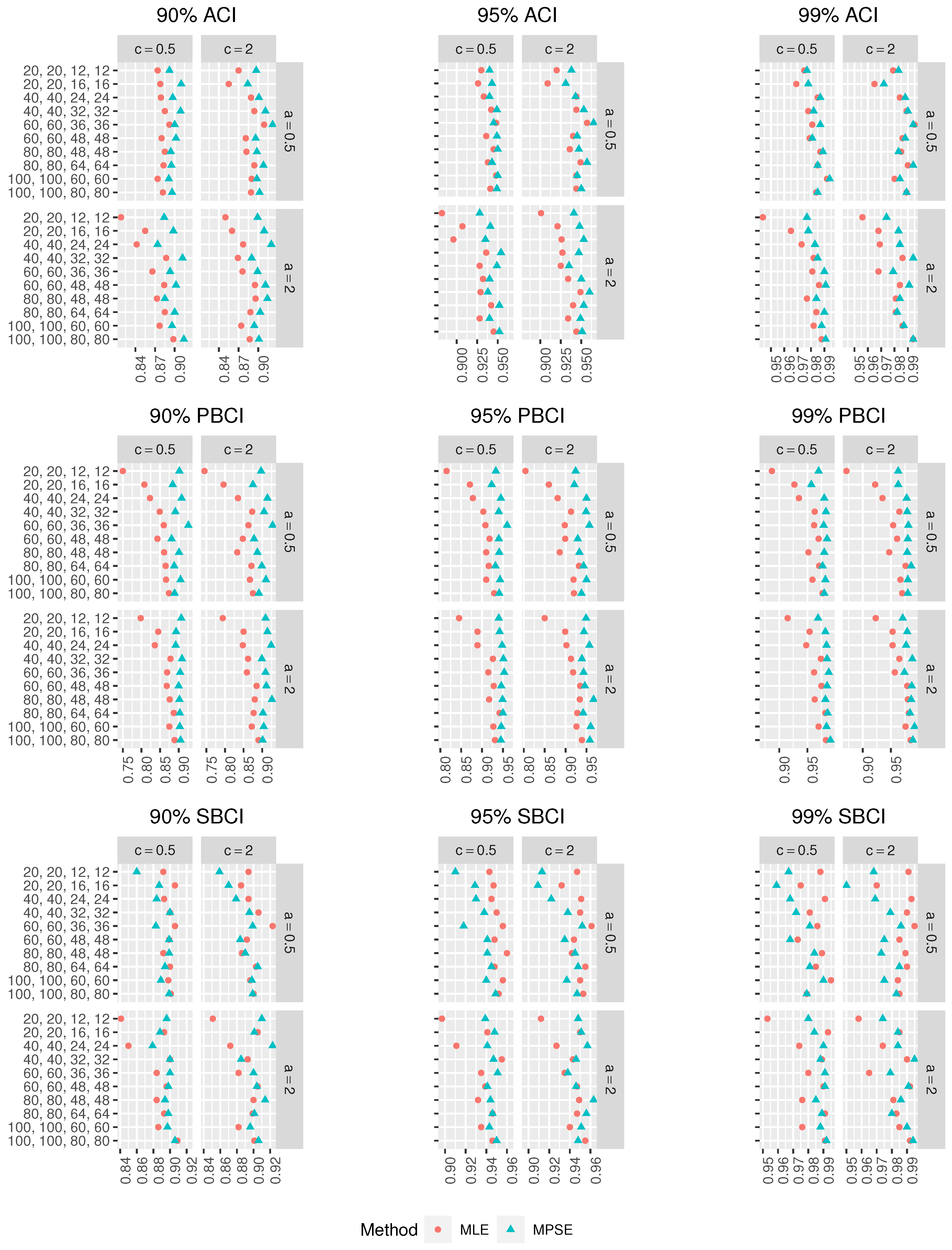
For each setting, the process was repeated 1000 times and the average values of biases and RMSEs for $a,b$ and c were obtained. These outcomes are displayed in Figure 3 and Figure 4, where Figure 3 displays the heatmaps of biases and Figure 4 presents the heatmaps of RMSEs. 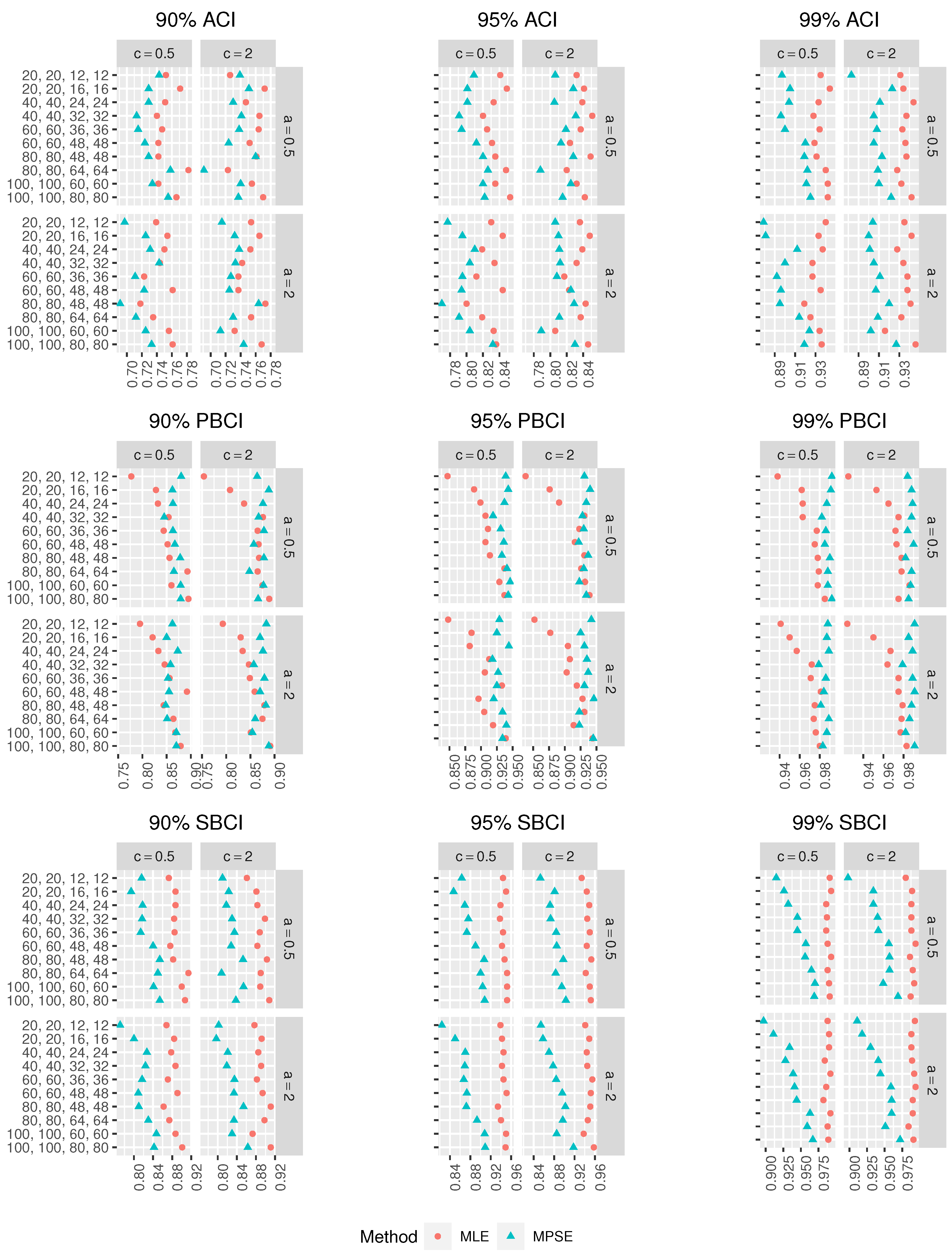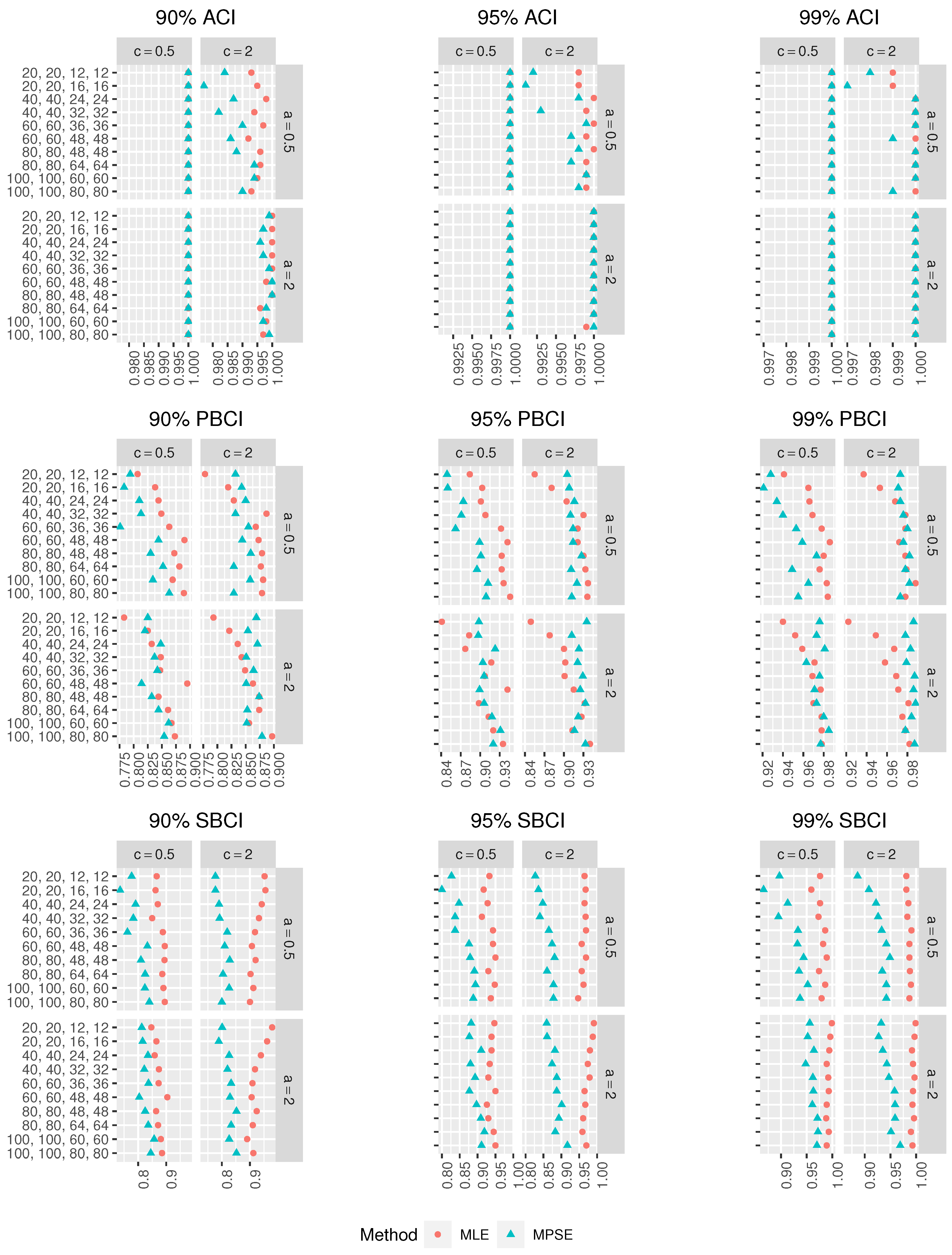In addition, to compare the performance of the different proposed confidence intervals (CIs), the lengths (Lens) of the CIs were computed and are presented in Figure 5, Figure 6 and Figure 7, respectively. In addition, the coverage probabilities (CPr) of the different CIs were obtained and are presented in Figure 8, Figure 9 and Figure 10. From the simulation results in Figure 3, Figure 4, Figure 5, Figure 6, Figure 7, Figure 8, Figure 9 and Figure 10, one can draw the following observations:

• For fixed $n_k,k=1,2$, as $r_k$ increases, the biases of the MLEs and MPSEs decrease, which implies that the estimators are asymptotically unbiased.
• For fixed $n_k,k=1,2$, as $r_k$ rises, the RMSEs of the MLEs and MPSEs decrease, which infers that the estimators are consistent.
• The MPSEs perform better than the MLEs based on minimum biases in all the cases.
• The MPSEs have fewer RMSEs than the MLEs in all the cases.
• For small $r_k,k=1,2$, the MPSEs have smaller biases and RMSEs than the MLEs in all the cases.
• In terms of minimum Lens, the different CIs based on the MPSEs perform better than those based on the MLEs.
• For fixed $n_k,k=1,2$, as $r_k$ increases, the Lens of the CIs using the MLEs and MPSEs decreases in all the cases.
• The ACIs based on the MLEs and MPSEs have the smallest Lens among other CIs in most of the cases.
• The ordering of performance for the CIs using the MLEs and MPSEs are the ACIs, SBCIs and PBCIs.
• In all the cases, as $r_k,k=1,2$, increases, the CPr of the different CIs tends to the nominal confidence level.
• Merging all the earlier results, we suggest using the MPS estimation method to estimate the parameters of the MKE distribution based on CSPALT and Type-II censored data.

7. Data Analysis Illustrative Examples

In this part of the paper, two data analysis examples are considered to show practical application of the estimation methods discussed in the preceding sections.

Example 1

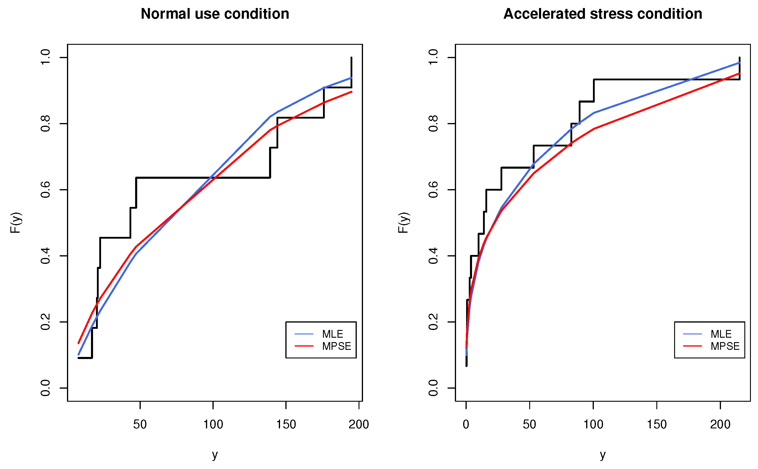
(Oil breakdown times of insulating fluid). The first data set to be analyzed is the oil breakdown times of insulating fluid subjected to different constant levels of high voltage. The main data set consists of additional observations since the tests were performed under different levels of stress, as reported in Nelson [35] and recently analyzed by many authors (see, for example, Nassar and Dey [2]). For the sake of illustration, the data set under stress level 30 kilo-volt (KV) was assumed to be the data under normal use conditions, while the observations under stress level 32 KV were considered to be the accelerated data set. The data sets of interest are provided in

Table 4. Oil breakdown observed times of insulating fluid, complete data.

Normal Use Condition (30 KV):

7.74, 17.05, 20.46, 21.02, 22.66, 43.40, 47.30, 139.07, 144.12, 175.88, 194.90

Accelerated Stress Condition (32 KV):

0.27, 0.40, 0.69, 0.79, 2.75, 3.91, 9.88, 13.95, 15.93, 27.80, 53.24, 82.85, 89.29, 100.58, 215.10

.

To analyze the data in Table 4, firstly, the goodness-of-fit of the MKE distribution was evaluated by using the one-sample Kolmogorov-Smirnov (K-S) test. The K-S statistic is obtained as follows:

$$\mathrm{K}-\mathrm{S}=\underset{1\le i\le n_k}{max}\left(F_k\left(y_{ki}\right)-\frac{i-1}{n_k},\frac{i}{n_k}-F_k\left(y_{ki}\right)\right),k=1,2.$$

The K-S distance and the corresponding p-value based on the MLEs and MPSEs are summarized in

Table 5. The MLEs, MPSEs and K-S statistics with the associated p-values for the oil breakdown, assuming complete data.

Condition	Estimator	a	b	KS	p-Value
Normal Use Condition	MLEs	0.8060	0.0078	0.22794	0.5432
	MPSEs	0.6832	0.0075	0.20797	0.6559
Accelerated Stress Condition	MLEs	0.4151	0.0161	0.14895	0.8463
	MPSEs	0.3663	0.0143	0.14783	0.8524

. Regardless of the considered estimator, the goodness-of-fit test indicates that the MKE distribution could be considered an adequate life model for the analyzed data set; nevertheless, MPSEs provided better goodness-of-fit outcomes. The empirical and fitted CDF plots of the MKE distribution for the data in Table 4 are depicted in Figure 11. For the sake of illustration, a Type-II censored CSPALT data set was obtained by considering $r_1=7$ and $r_2=10$. Accordingly, the MLEs and MPSEs and the associated standard errors were acquired for the model parameters as well as the considered $95\%$ CIs, as shown in

Table 6. The MLEs, MPSEs and the corresponding standard errors (in parentheses) and the different $95\%$ CIs for the oil breakdown Type-II censored CSPALT data.

Method	a	b	c
MLEs	0.8024(0.193)	0.0139(0.005)	3.2067(1.984)
ACIs	(0.427, 1.178)	(0.004, 0.024)	(1.000, 7.096)
PBCIs	(0.492, 2.301)	(0.008, 0.039)	(1.262, 20.23)
SBCIs	(0.298, 1.309)	(0.003, 0.028)	(1.000, 4.874)
MPSEs	0.6281(0.163)	0.0118(0.006)	2.3484(1.402)
ACIs	(0.309, 0.947)	(0.001, 0.023)	(1.000, 5.096)
PBCIs	(0.295, 1.228)	(0.005, 0.036)	(1.000, 3.787)
SBCIs	(0.000, 0.919)	(0.000, 0.023)	(1.000, 3.114)

. Based on the outcomes of the latter table, one can observe that the MPSEs of the parameters a and c perform better than the MLEs in terms of minimum standard errors, while the MLE of the parameter b has a smaller standard error than the MPSE. On the other hand, the CIs computed via the MPSEs have a slightly shorter interval Lens than those obtained based on the MLEs, and similarly, the ACIs have slightly smaller interval lengths among other CIs, except in some cases. Based on the MLEs and MPSEs displayed in Table 6, the estimates of the mean time to failure (MTTF) and RF using some mission times under normal use conditions were obtained and are displayed in

Table 7. The MLEs and MPSEs of the MTTF and RF for the oil breakdown Type-II censored CSPALT data.

Method	MTTF	${\mathit{R}}_{\mathbf{1}}\mathbf{\left(}\mathbf{10}\mathbf{\right)}$	${\mathit{R}}_{\mathbf{1}}\mathbf{\left(}\mathbf{20}\mathbf{\right)}$	${\mathit{R}}_{\mathbf{1}}\mathbf{\left(}\mathbf{50}\mathbf{\right)}$
MLEs	43.808	0.8048	0.6695	0.3668
MPSEs	54.130	0.7625	0.6470	0.4181

.

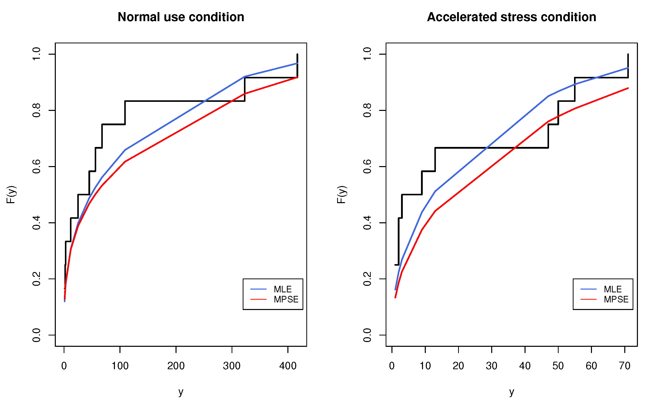
Example 2

(Time to breakdown of steel specimens). The second data set was reported by Nelson [35]. The data consist of the time to breakdown of steel specimens under different stress levels. The data sets under stress levels of 40 KV (normal use) and 45 KV (accelerated stress), each containing 12 observations, are listed in

Table 8. Time to breakdown of steel specimens, complete data.

Normal Use Condition (40 KV):

1, 1, 2, 3, 12, 25, 45, 56, 68, 109, 323, 417

Accelerated Stress Condition (45 KV):

1, 1, 1, 2, 2, 3, 9, 13, 47, 50, 55, 71

. Before analyzing this data, we checked the validity of the MKE model to fit the two data sets. The MLEs, MPSEs and K-S and the corresponding p-value were obtained and are listed in

Table 9. The MLEs, MPSEs and K-S statistics with the associated p-values for the breakdown of steel, complete data.

Condition	Estimator	a	b	KS	p-Value
Normal Use Condition	MLEs	0.4176	0.0072	0.18718	0.79450
	MPSEs	0.3863	0.0059	0.21841	0.61610
Accelerated Stress Condition	MLEs	0.5074	0.0322	0.23105	0.54350
	MPSEs	0.5191	0.0233	0.27436	0.32700

. It is seen from the results in Table 9 that the MKE distribution could be accepted as a fit model for the given data sets. The empirical and fitted CDF plots of the MKE distribution for the data in Table 8 are displayed in Figure 12.

From the complete data sets in Table 8, a Type-II censored CSPALT data set was considered by choosing $r_1=r_2=8$. Consequently, the MLEs and MPSEs and the associated standard errors were obtained and are reported in

Table 10. The MLEs, MPSEs and the corresponding standard errors (in parentheses) and the different $95\%$ CIs for the breakdown of steel Type-II censored CSPALT data.

Method	a	b	c
MLEs	0.61830 (0.01823)	0.01376 (0.00003)	2.98191 (2.56567)
ACIs	(0.35369, 0.88291)	(0.00272, 0.02480)	(1.00000, 6.12132)
PBCIs	(0.39397, 1.59171)	(0.00802, 0.04358)	(1.84773, 17.10302)
SBCIs	(0.27484, 0.99224)	(0.00093, 0.02838)	(1.03927, 4.61020)
MPSEs	0.51429 (0.02089)	0.01037 (0.00004)	1.83031 (1.28120)
ACIs	(0.23104, 0.79755)	(0.00000, 0.02201)	(1.0000, 4.04879)
PBCIs	(0.25990, 0.95612)	(0.00436, 0.04049)	(1.21514, 3.09663)
SBCIs	(0.00000, 0.79302)	(0.00000, 0.02015)	(0.67398, 2.64974)

. In addition, the different $95\%$ CIs of the unknown parameters were evaluated and are displayed in Table 10. From the tabulated outcomes given in Table 10, it is noted that CIs evaluated based on the MPSEs had the smallest Lens in most of the cases, especially when estimating the parameters b and c, and the bootstrap CIs based on the MPSEs performed better than the ACIs in terms of CIs Lens, except for in the case when estimating the parameter a. Using the MLEs and MPSEs presented in Table 10, the MLEs and MPSEs of the MTTF and RF using mission times under normal use conditions were obtained and are displayed in

Table 11. The MLEs and MPSEs of the MTTF and RF for the breakdown of steel Type-II censored CSPALT data.

Method	MTTF	${\mathit{R}}_{\mathbf{1}}\mathbf{\left(}\mathbf{5}\mathbf{\right)}$	${\mathit{R}}_{\mathbf{1}}\mathbf{\left(}\mathbf{20}\mathbf{\right)}$	${\mathit{R}}_{\mathbf{1}}\mathbf{\left(}\mathbf{50}\mathbf{\right)}$
MLEs	46.61	0.8226	0.6118	0.3702
MPSEs	65.532	0.8015	0.6249	0.4405

.

8. Conclusions

In this paper, investigation of the constant-stress partially accelerated life test, where the lifetime of the experimental units is obtained from the modified Kies exponential distribution, is considered. Based on Type-II censored data, the maximum likelihood and maximum product of spacing estimates of the unknown parameters are obtained. Furthermore, using both estimation methods, the approximate confidence intervals of the unknown parameters are built using the observed Fisher information matrix. In addition, two parametric bootstrap confidence intervals based on both approaches are additionally given for comparison objects. The efficiency of the various point and interval estimators is examined via simulation studies. Two real data sets are considered to show the applicability of the methods employed in this paper. The simulation and real data analysis outcomes show that the maximum product of spacing provides better estimates than their conventional counterparts derived using the maximum likelihood approach.

References

1. Yin, Y.C.; Coolen, F.P.; Coolen-Maturi, T. An imprecise statistical method for accelerated life testing using the power-Weibull model. Reliab. Eng. Syst. Saf. 2017, 167, 158–167. [Google Scholar] [CrossRef]
2. Nassar, M.; Dey, S. Different estimation methods for exponentiated Rayleigh distribution under constant-stress accelerated life test. Qual. Reliab. Eng. Int. 2018, 34, 1633–1645. [Google Scholar] [CrossRef]
3. Dey, S.; Nassar, M. Classical methods of estimation on constant stress accelerated life tests under exponentiated Lindley distribution. J. Appl. Stat. 2020, 47, 975–996. [Google Scholar] [CrossRef]
4. Sief, M.; Liu, X.; Abd El-Raheem, A.E. Inference for a constant-stress model under progressive type-I interval censored data from the generalized half-normal distribution. J. Stat. Comput. Simul. 2021, 91, 3228–3253. [Google Scholar] [CrossRef]
5. Balakrishnan, N.; Kundu, D.; Ng, K.T.; Kannan, N. Point and interval estimation for a simple step-stress model with Type-II censoring. J. Qual. Technol. 2007, 39, 35–47. [Google Scholar] [CrossRef]
6. El-Din, M.M.; Abu-Youssef, S.E.; Aly, N.S.; Abd El-Raheem, A.M. Estimation in step-stress accelerated life tests for Weibull distribution with progressive first-failure censoring. J. Stat. Appl. Probab. 2014, 3, 403. [Google Scholar]
7. Nassar, M.; Okasha, H.; Albassam, M. E-Bayesian estimation and associated properties of simple step–stress model for exponential distribution based on type-II censoring. Qual. Reliab. Eng. Int. 2021, 37, 997–1016. [Google Scholar] [CrossRef]
8. Guan, Q.; Tang, Y.; Fu, J.; Xu, A. Optimal multiple constant-stress accelerated life tests for generalized exponential distribution. Commun.-Stat. Comput. 2014, 43, 1852–1865. [Google Scholar] [CrossRef]
9. Mohie El-Din, M.M.; Abu-Youssef, S.E.; Ali, N.S.; Abd El-Raheem, A.M. Classical and Bayesian inference on progressive-stress accelerated life testing for the extension of the exponential distribution under progressive type-II censoring. Qual. Reliab. Eng. Int. 2017, 33, 2483–2496. [Google Scholar] [CrossRef]
10. Bagdonavicius, V.; Nikulin, M. Accelerated Life Models: Modeling and Statistical Analysis; CRC Press: New York, NY, USA, 2001. [Google Scholar]
11. Mahmoud, M.A.; EL-Sagheer, R.M.; Abou-Senna, A.M. Estimating the Modified Weibull Parameters in Presence of Constant-Stress Partially Accelerated Life Testing. J. Stat. Theory Appl. 2018, 17, 242–260. [Google Scholar] [CrossRef] [Green Version]
12. Dey, S.; Wang, L.; Nassar, M. Inference on Nadarajah–Haghighi distribution with constant stress partially accelerated life tests under progressive type-II censoring. J. Appl. Stat. 2021, 1–22. [Google Scholar] [CrossRef]
13. Ahmadini, A.A.H.; Mashwani, W.K.; Sherwani, R.A.K.; Alshqaq, S.S.; Jamal, F.; Miftahuddin MAbbas, K.; Razaq, F.; Elgarhy, M.; Al-Marzouki, S. Estimation of Constant Stress Partially Accelerated Life Test for Fréchet Distribution with Type-I Censoring. Math. Probl. Eng. 2021, 9957944. [Google Scholar] [CrossRef]
14. Li, X.; Zheng, H. Estimation and optimum constant-stress partially accelerated life test plans for Gompertz distribution with Type-I censoring. Commun.-Stat.-Theory Methods 2015. [Google Scholar] [CrossRef]
15. Al-Babtain, A.A.; Shakhatreh, M.K.; Nassar, M.; Afify, A.Z. A new modified Kies family: Properties, estimation under complete and type-II censored samples, and engineering applications. Mathematics 2020, 8, 1345. [Google Scholar] [CrossRef]
16. Almetwally, E.M.; Alharbi, R.; Alnagar, D.; Hafez, E.H. A new inverted topp-leone distribution: Applications to the COVID-19 mortality rate in two different countries. Axioms 2021, 10, 25. [Google Scholar] [CrossRef]
17. Abd El-Raheem, A.M.; Almetwally, E.M.; Mohamed, M.S.; Hafez, E.H. Accelerated life tests for modified Kies exponential lifetime distribution: Binomial removal, transformers turn insulation application and numerical results. AIMS Math. 2021, 6, 5222–5255. [Google Scholar] [CrossRef]
18. Aljohani, H.M.; Almetwally, E.M.; Alghamdi, A.S.; Hafez, E.H. Ranked set sampling with application of modified Kies exponential distribution. Alex. Eng. J. 2021, 60, 4041–4046. [Google Scholar] [CrossRef]
19. Lawless, J.F. Statistical Models and Methods for Lifetime Data; John Wiley & Sons: Hoboken, NJ, USA, 2003. [Google Scholar]
20. Cheng, R.C.H.; Amin, N.A.K. Estimating parameters in continuous univariate distributions with a shifted origin. J. R. Stat. Soc. Ser. B (Methodol.) 1983, 45, 394–403. [Google Scholar] [CrossRef]
21. Ranneby, B. The maximum spacing method. An estimation method related to the maximum likelihood method. Scand. J. Stat. 1984, 11, 93–112. [Google Scholar]
22. Anatolyev, S.; Kosenok, G. An alternative to maximum likelihood based on spacings. Econom. Theory 2005, 21, 472–476. [Google Scholar] [CrossRef] [Green Version]
23. Ng, H.K.T.; Luo, L.; Hu, Y.; Duan, F. Parameter estimation of three-parameter Weibull distribution based on progressively type-II censored samples. J. Stat. Comput. Simul. 2012, 82, 1661–1678. [Google Scholar] [CrossRef]
24. R Core Team. R: A Language and Environment for Statistical Computing; R Foundation for Statistical Computing: Vienna, Austria, 2020. [Google Scholar]
25. MacDonald, I.L. Does Newton–Raphson really fail? Stat. Methods Med. Res. 2014, 23, 308–311. [Google Scholar] [CrossRef] [PubMed]
26. Fox, P.A.; Hall, A.P.; Schryer, N.L. The PORT mathematical subroutine library. ACM Trans. Math. Softw. (TOMS) 1978, 4, 104–126. [Google Scholar] [CrossRef]
27. Nassar, M.; Dey, S.; Kumar, D. A new generalization of the exponentiated Pareto distribution with an application. Am. J. Math. Manag. Sci. 2018, 37, 217–242. [Google Scholar] [CrossRef]
28. Basu, S.; Singh, S.K.; Singh, U. Bayesian inference using product of spacings function for Progressive hybrid Type-I censoring scheme. Statistics 2018, 52, 345–363. [Google Scholar] [CrossRef]
29. Ghosh, K.; Jammalamadaka, S.R. A general estimation method using spacings. J. Stat. Plan. Inference 2001, 93, 71–82. [Google Scholar] [CrossRef] [Green Version]
30. Basu, S.; Singh, S.K.; Singh, U. Parameter estimation of inverse Lindley distribution for Type-I censored data. Comput. Stat. 2017, 32, 367–385. [Google Scholar] [CrossRef]
31. Basu, S.; Singh, S.K.; Singh, U. Estimation of inverse Lindley distribution using product of spacings function for hybrid censored data. Methodol. Comput. Appl. Probab. 2019, 21, 1377–1394. [Google Scholar] [CrossRef]
32. Efron, B. The Jackknife, the Bootstrap and Other Resampling Plans; CBMS-NSF Monographs 38; Society for Industrial and Applied Mathematics: Philadelphia, PA USA, 1982. [Google Scholar]
33. Hall, P. Theoretical comparison of bootstrap confidence intervals. Ann. Stat. 1988, 16, 927–953. [Google Scholar] [CrossRef]
34. Nash, J.C. On best practice optimization methods in R. J. Stat. Softw. 2014, 60, 1–14. [Google Scholar] [CrossRef] [Green Version]
35. Nelson, W.B. Accelerated Testing: Statistical Model, Test Plan and Data Analysis; Wiley: New York, NY, USA, 2004. [Google Scholar]
Figure 1. Plots of PDF, CDF, RF and HRF of the MKE distribution.
Mathematics 10 00819 g001
Figure 2. Four-dimensional profiling of the objective functions for complete sample (upper panel) and Type-II censored sample (lower panel).
Mathematics 10 00819 g002
Figure 3. The heatmaps of the simulated biases of the MLEs and MPSEs of a , b and c.
Mathematics 10 00819 g003
Figure 4. The heatmaps of the simulated RMSEs of the MLEs and MPSEs of a , b and c.
Mathematics 10 00819 g004
Figure 5. Simulated Lens of different CIs of a.
Mathematics 10 00819 g005
Figure 6. Simulated Lens of different CIs of b.
Mathematics 10 00819 g006
Figure 7. Simulated Lens of different CIs of c.
Mathematics 10 00819 g007
Figure 8. Simulated CPr of different CIs of a.
Mathematics 10 00819 g008
Figure 9. Simulated CPr of different CIs of b.
Mathematics 10 00819 g009
Figure 10. Simulated CPr of different CIs of c.
Mathematics 10 00819 g010
Figure 11. The empirical and fitted CDF of the MKE distribution for oil breakdown data.
Mathematics 10 00819 g011
Figure 12. The empirical and fitted CDF of the MKE distribution for the breakdown of steel data.
Mathematics 10 00819 g012