Abstract
The immune system is the body’s defense against pathogens, which are complex living organisms found in many parts in the body including organs, tissues, cells, molecules, and proteins. When the immune system works properly, it can recognize and kill the abnormal cells and the infected cells. Otherwise, it can attack the body’s healthy cells even if there is no invader. Many researchers have developed immunotherapy (or cancer vaccines) and have used chemotherapy for cancer treatment that can kill fast-growing cancer cells or at least slow down tumor growth. However, chemotherapy drugs travel throughout the body and tend to kill both healthy cells and cancer cells. In this study, we consider the fact that chemotherapy can kill tumor cells and that the loss of the immune cells may at the same time stir up cancer growth. We present a dynamic time-delay tumor-immune model with the effects of chemotherapy drugs and autoimmune disease. The modeling results can be used to determine the progression of tumor cells in the human body with the effect of chemotherapy, autoimmune diseases, and time delays based on partial differential equations. It can also be used to predict when the tumor viruses’ free state can be reached as time progresses, as well as the state of the body’s healthy cells as time progresses. We also present a few numerical cases that illustrate that the model can be used to monitor the effects of chemotherapy drug treatment and the growth rate of tumor virus-infected cells and the autoimmune disease.
Keywords:
immune system; tumor virus; effector cell; autoimmune disease; time-delay virus-immune model; chemotherapy drug MSC:
35-00; 90-00
1. Introduction
Human beings are constantly exposed to germs such as bacteria and viruses that enter the human body and eventually make people sick. One of the tasks of the body’s immune system is to fight off infections, prevent viruses and germs from entering the body, and destroy any infectious microorganisms that do invade the body [1,2,3].
The skin is a part of the immune system that prevents germs from entering the body [4]. When the body senses danger from a virus or infection, the immune system will respond and attack it. Many researchers have developed immunotherapy and chemotherapy to improve the ability of the immune system and cancer treatment, respectively, to attack cancer cells. When chemotherapy drugs are injected into a person, they travel throughout the body, a process during which they can also damage healthy cells. The loss of the immune cells may at the same time stir up cancer growth.
The human immune system is complex, and the body’s defense system, which consists of various cells, tissues, molecules, and organs, works together to defend the body and fight the infections when germs enter it [1,2,5]. When our immune system learns about any germs or viruses after we have been exposed to them, it will develop antibodies to protect us from those specific germs [1,6]. When our immune system doesnot work properly, it is called an autoimmune disease, in which the body, unfortunately, attacks healthy cells when there is no invader [1,5].
The interest in the development of mathematical models in cancer epidemiology [7,8,9,10] and infectious disease epidemiology [11,12] to predict the growth of tumors and cancer cells has seen a dramatic upswing in recent decades. Many models [9,10,13,14,15,16] have been developed using partial differential equations in the past and delay partial differential equations have been used in recent years to characterize tumor-immune dynamic growth. However, there is still no consensus on the modeling due to the complexity of virus-infected and tumor cancer growth in the body’s immune system and the growth patterns of the tumors and infected cells [16]. Many researchers [7,17,18,19,20,21,22,23,24] have used the existing prey–predator modeling concept [25,26] to study and model tumor–immune interactions [7,27,28] and the effects of tumor growth [17,29,30]. Huniti et al. [17], for example, presented a review of recent research in the area of tumor growth dynamic modeling and the mixture of tumor growth dynamic modeling of immuno-oncology and chemotherapy agents based on partial differential equations. Unlike chemotherapy, patients with immunotherapy demonstrate unique tumor dynamics profiles in which tumor shrinkage occurs at the beginning but then is maintained at the steady-state tumor level for a long time with stable disease [17].
Modeling studies of prey–predator systems and their related applications have seen a tremendous amount of interest in recent years in various disciplines, including population disease [31,32], life expectancy [33,34], biomathematics [35,36], cancel growth [29,37,38,39,40,41,42], and engineering science [23,35,43]. Many researchers have studied various dynamic prey–predator models including multi-dimension predator-prey models [44,45,46,47,48,49], multi-prey models [50,51,52], and time-delay prey–predator models [23,36,43,50] with various applications in biomathematics [53], population disease [22,23,29,30,54,55,56,57,58,59], and recent COVID-19 disease analysis [1,12,60,61,62,63,64,65,66]. Haque et al. [54] analyzed a predator–prey model using standard disease incidence. Naji and Mustafa [56] studied a dynamic model of eco-epidemiology concerning nonlinear disease incidence rates with an infective type of disease in prey. Mukhopadhyaya and Bhattacharyya [36] studied the modeling effect of a prey–predator delay model with disease using a Holling type II functional response. Wang et al. [43] studied a distributed predator–prey delay model. Huang et al. [22] recently studied a stochastic predator–prey model with a Holling II increasing function in the predator.
Jana and Kar [23] studied an epidemiological dynamic model incorporating time delay by considering a susceptible prey becoming infected. Lestari et al. [29] discussed a mathematical model of the spread of tumor cancellation with chemotherapy based on partial differential equations. They numerically determined the growth rate of cancer cells. Pham [63] studied a model to predict the number of COVID-19 deaths based on the US data, and recently, Pham [64] studied the effects of several COVID-19 pandemic restrictions including reopening states, social distancing, reopening schools, and face mask mandates in the modeling. Pham and Pham [65] discussed a model to predict the presence of breast cancer based on biomarkers. Kiddy et al. [66] recently formulated a new deterministic model to capture the dynamics of the COVID-19 disease in Ghana and Egypt using various compartmental variables such as susceptible, exposed, asymptomatic, quarantined asymptomatic, severely infected, hospitalized, recovered, recovered asymptomatic, deceased, and protective susceptible with a standard incidence rate. They noticed that the number of undetected recoveries overpasses the number of detected recoveries for the proposed countries. Pham [67] recently discussed a virus-immune time-delay model of virus-infected cells and immune system but did not consider a chemotherapy drug treatment. Further research study of the time delay between the virus infection, tumor cell growth, and chemotherapy drug treatment is crucial in determining how long the current growth could continue before the slowdown owing to a newly-introduced intervention of chemotherapy treatment becoming visible. This paper aims to extend Pham’s work [67] by considering the effects of time-delay chemotherapy drug treatment. In other words, this paper studies the mathematical modeling of the time-delay interactions between tumor cells and the immune system and the effects of chemotherapy and autoimmune diseases. The model can be used to determine the dynamic progression of tumor cell growth and observe the patterns of how the tumor viruses spread in the body’s immune system with respect to time delays. In Section 2, we discuss the model’s assumptions and mathematical formulation of the model. Section 3 discusses several numerical examples to illustrate the modeling results. Section 4 discusses brief conclusions and presents future research problems.
2. A Mathematical Model with Multiple Time Delays between Tumor Viruses and Effector Cells
In this section, we discuss a time-delay model consisting of three partial differential equations including a growth rate of immune cells, growth rate of tumor cells, and growth amount of the concentration of chemotherapy drug based on a recent work by the author [67]. Although many assumptions below can be found in [29,67], for the sake of convenience, we will list them here as well.
Notation
We use the following notation, partially from [67], throughout the paper:
a = the intrinsic growth rate per unit time
b = the elimination rate of the tumor cells by the healthy immune system (effector cells) per cells and unit time
c = the death rate of the healthy immune system per unit time
d = degree of recruitment of maximum immune-effector cells in relation with tumor cells per unit time
e = capacity of the tumor cells per unit time
f = the rate that the immune system attacks the body’s own healthy (effector) cells, resulting in autoimmune disease per cells and unit time
g = constant factor of growth rate per unit time
h = the half saturation constant (cells)
k = the half saturation for tumor cleanup (cells)
m = the degree of inactivation of effector cells by tumor cells per cells and unit time
p = parameter of tumor cells cleanup by immune-effector cells per unit time
s = growth rate of immune-effector cells per unit time
I(t) = the number of healthy immune-effector cells at time t
V(t) = the number of tumor cells at time t
Q(t) = the amount of the concentration of chemotherapy drug
α = rate of decrease in concentration of chemotherapy drug
β = the occurrence of a drug from outside the body
β(t) = the amount of chemotherapy drug injected to a patient at a given time
r = rate of the influence of the interaction between effector cells and the chemotherapy drug
u = rate of the influence of the interaction between tumor cells and the chemotherapy drug.
2.1. Immune Cell Time-Delay Model Formulation
In the population of healthy immune-cell or effector cells, we assume that:
- The effector cell has a constant growth rate, s, of effector cells [29,67].
- The effector cell has a natural death rate, c, of effector cells
- There is an increase in effector cells by the growth rate d with a degree of recruitment of maximum immune-effector cells of the response of toward tumor cells [29] with a time delay
- There is a constant rate f when the immune system attacks the body’s own healthy (effector) cells, resulting in autoimmune disease [67]. The constant f, in general, will be very small compared to c, so that when I is not too large, then the term f I2 will be negligible compared to cI.
- There will be a reduced number of effector cells due to their interactions with tumor cells having a constant rate m [29], and the chemotherapy drug damage the effector cells with rate of r.
Based on Assumption 5 and [67], a model of the rate of the immune effector cells governing the interactions between the tumor cells, immune cells, and chemotherapy over time can be presented:
2.2. Tumor Cells Time-Delay Model Formulation
In the population of tumor cells, which is when a cancer virus infects a host, it invades the healthy immune cells of its host and also can infect other cells, we assume that:
- 6.
- The tumor cell has a constant growth rate, a [29], considering a constant factor of growth rate, g, and a time delay before the tumor virus infects the cell [67].
- 7.
- There will be a constant elimination rate of the tumor cells by the healthy immune system (effector cells), b, by a time delay. In other words, b measures how efficiently effector cells kill tumor cells.
- 8.
- The tumor cells willdecline by a constant parameter of tumor cleanup of effector cells, p [29], with a time delay.
- 9.
- There will be a reduction in the number of the tumor cells by a constant rate e that occurs becausethere are two virus cells per unit time competing with each other due to the limited number of host cells. The constant rate e here can be considered to be very small.
- 10.
- There will be a reduction in the number of tumor cells due to the influence of the interaction between tumor cells and the chemotherapy drug with a rate u.
From Assumption (10), we can derive a mathematical equation as follows:
Based on Assumptions 6–10 and [67], a model of the rate of the tumor virus cells can be presented as follows:
2.3. The Concentration of Chemotherapy Drug over Time
The assumptions of the rate of change in the amount of the concentration of chemotherapy drug over the time-delay are assumed as follows:
- 11.
- The amount of the concentration of chemotherapy drug increases with a rate of β because of the occurrence of the chemotherapy drug.
- 12.
- The amount of the chemotherapy drug concentration would decrease with a rate of α over the timedelay.
Based on Assumptions 11 and 12, we can present the following mathematical differential equation:
Thus, from Equations (1), (3), and (4), a new tumor-immune time-delay model based on [67] for the body’s immune system, with considerations of multiple interactions between the tumor virus cells, body’s immune cells with autoimmune disease, and chemotherapy, is as follows:
In this study, we consider the amount of chemotherapy drug injected into a patient at a given time to be constant, that is, β(t) = β. Note that the model studied by Lestari et al. [29] is a special case of our model as given from Equation (5) where f = 0, e = 0, g = 0, τ1 = 0, τ2 = 0, and τ3 = 0. In addition, when r = 0, u = 0, α = 0, and β = 0, it yields the model in [67].
We now wish to determine the number of immune-infector cells I(t), tumor virus cells V(t), and the concentration of chemotherapy drug Q(t) at any given time. We develop a program using R software to calculate and plot the functions I(t), V(t), and Q(t) with respect to time t as will be discussed in the next section.
3. Modeling Results
We now present a numerical analysis of the proposed model. Table 1 shows the parameter values that we use in our analysis based on existing studies [29,39,40,41,67] for the illustration of our model. Any other sets of parameter values can be easily applied from the model.

Table 1.
Model parameter values.
Here, we consider various initial numbers of tumor virus cells and the number of immune-effect cells to be from 15,000 to 30,000 and from 50,000 to 75,000, respectively, to explore if the results depend on those initial number of cells in solving the partial differential equations. Below, we discuss several cases based on various parameter values of the tumor virus growth rates, a, the elimination rate of the tumor virus cells by the immune-effector cells, b, and a growth rate of immune-effector cells, s, as follows:
Case 1: s = 7000
We first assume that the initial number of tumor virus cells is V0 = 30,000, the initial number of immune-effector cells is I0 = 75,000, and the concentration of chemotherapy drug is Q0 = 0. From Figure 1a–c, we can observe that the initial numbers of tumor virus cells, immune-effector cells, and concentration of chemotherapy drug are 30,000, 75,000, and 0, respectively, as expected. The tumor virus-infected counts begin to increase only upto the fourth day and then start to decrease until they reach the lowest number of tumor cells at around 23,360, which is at about the 18th day. Then, the counts begin to increase until they slowly stabilize at around 31,885 after around the 275th day (see Figure 1a in red). As seen in Figure 1b (in blue), the number of immune-effector cells keeps increasing but starts to slowly stabilize after the 170th day at the level of 90,578. Figure 1c (in green) shows the concentration of the chemotherapy drug versus the time (day). It seems that in this case, with a given growth rate of effector cells s = 7000 cells per day and the tumor virus growth rate a = 0.43, it will not be able to reach the tumor virus-free state. Figure 1d–f show the relationship between the immune-effector cells and tumor cells.
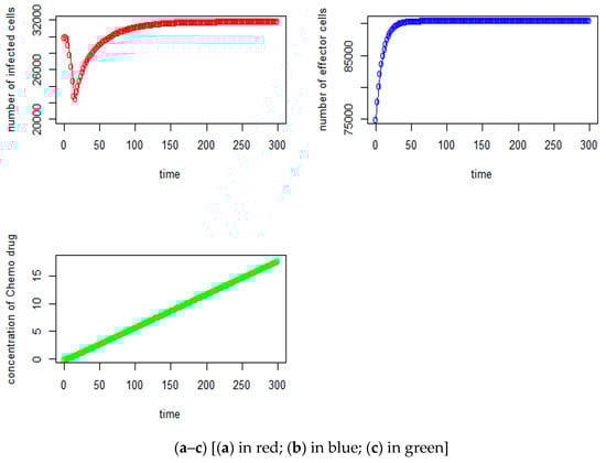
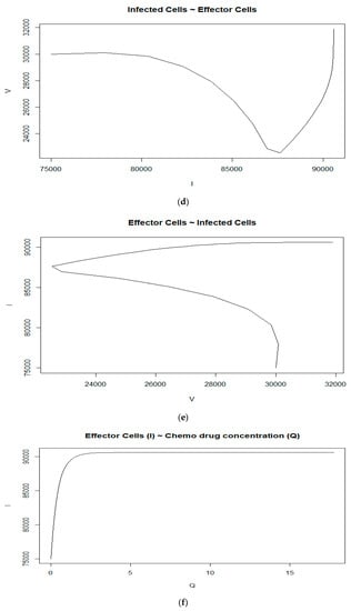
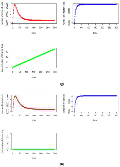
Figure 1.
(a) Tumorvirus-infected cells, (b) immune-effector cells and (c) concentration of chemo drug versus time (days); (d) the relationship between the tumor virus-infected cells and immune-effector cells; (e) the immune-effector cells versus tumor virus-infected cells; (f) the relationship between the immune-effector cells and the concentration of chemotherapy drug; (g) (no time delay case): (in red)tumor virus-infected cells, (blue) the immune-effector cells and (green) concentration of chemo drug versus time (days); (h) (no chemotherapy drug case): (red) tumor virus-infected cells, (blue) the immune-effector cells, and (green) concentration of chemo drug versus time (days).
Case 1A (No time delays): s = 7000, τI = 0, τ2 = 0, τ3 = 0, τ4 = 0, τ5 = 0
Here we assume that there are no time delays (i.e., τI = 0, τ2 = 0, τ3 = 0, τ4 = 0, τ5 = 0). Using Equation (5),we can observe that the number of tumor-infected cells significantly increases and it reaches the highest number of tumor cell counts at around 43,000, which is about the 8th day, given that the initial tumor cells was 30,000 and starts to decrease andstabilizes at the level of initial tumor cells. It will not reach down to the level of tumor infected free state as shown in Figure 1g.
For the time delay case (see Figure 1a), it is the opposite direction as it first decreases and then increases, whereas for the non-time delay, it will first increase and then decrease the number of tumor cells.
Case 1B (With time delays but no chemotherapy drug): s = 7000, r = 0, u = 0, α = 0, β = 0
The result for this case is about the same as with Case 1A, except the tumor-infected cells will reach the highest number of tumor cells at around 42,900 on the 10th day (see Figure 1h).
We observe that the model provides the same results for various initial numbers of immune effector cells and tumor cells as shown in Figure 2, Figure 3 and Figure 4. This indicates that the initial numbers of tumor cells and immune-effector cells do not influence the end results, whether they are tumor-virus-free or not. This shows an important result, namely that our model can be used to obtain the results without the need to know the exact initial number of tumor virus cells or the number of immune effector cells in the body.
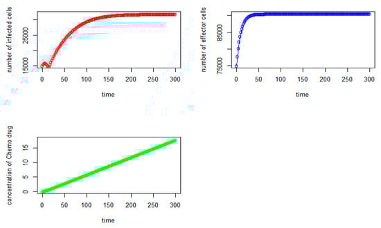
Figure 2.
Tumor virus-infected cells (red), immune-effector cells (blue) and concentration of chemo drug (green) versus time (days) for the initial values: V = 15,000, I = 75,000, Q = 0).
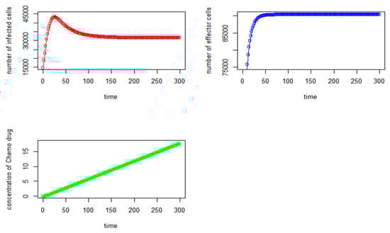
Figure 3.
Tumor virus-infected cells (red), immune-effector cells (blue), and concentration of chemo drug (green) versus time (days) for the initial values: V = 15,000, I = 50,000, Q = 0).
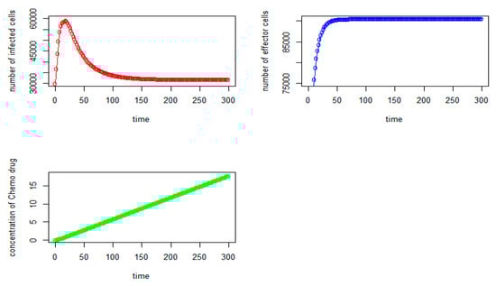
Figure 4.
Tumor virus-infected cells (red), immune-effector cells (blue), and concentration of chemo drug (green) versus time (days) for the initial values: V = 30,000, I = 50,000, Q = 0).
Case 2: This is the same as Case 1 except s = 10,000 (instead of s = 7000).
From Figure 5, we can observe that the initial number of tumor virus-infected cells and immune-effector cells are 30,000 and 75,000, respectively, as expected. It should be noted that the number of immune-effector cells (see Figure 5, in blue) keeps increasing but starts to slowly stabilize after the 70th day at the level of 114,910. The tumor virus-infected counts (see Figure 5, in red) begin to increase, and it reaches the highest point at around the 3rd day with (V,I) = (30,087, 83,358) and immediately starts to decrease significantly until it reaches the tumor virus-free state at (V,I) = (0, 114,790) after the 280th day, where the number of immune-effector cells is 114,790 and the concentration of thechemo drug level is about 16.57. When we do not consider the time delays in the modeling (see Equation (8)), that is,τI = 0, τ2 = 0, τ3 = 0, τ4 = 0, τ5 = 0, the tumor cells will grow quickly from the beginning, and it reaches the highest point at around the 4th day with about 34,000 tumor cells. With chemotherapy and the large number of immune-effector cells, the number of tumor cells begins to decrease significantly, and it reaches the tumor-cell-free state after the 190th day, and the immune-effector cells start to slowly stabilize after the 60th at the level of 114,800, as shown in Figure 6.
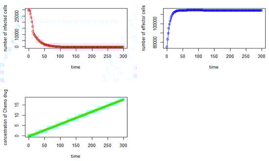
Figure 5.
Tumor virus-infected cells (red), immune-effector cells (blue), and concentration of chemo drug (green) versus time (days) (same as Figure 1 except s = 10,000).

Figure 6.
(No time delay case): tumor virus-infected cells (red), immune-effector cells (blue), and concentration of chemo drug (green) versus time (days).
Figure 7, Figure 8 and Figure 9 show various initial numbers of tumor virus-infected cells, such as 30,000 and 15,000, and immune-effector cells, such as 50,000 and 70,000. We observe that the tumor virus-infected counts first increase and immediately start to decrease significantly until they reach the tumor virus-free state as shown in Figure 7, Figure 8 and Figure 9. It is worth noting that the initial numbers of tumor virus-infected cells and immune-effector cells do not influence the end results.

Figure 7.
Tumor virus-infected cells (red), the immune-effector cells (blue), and concentration of chemo drug (green) versus time (days) for the initial values: V = 15,000, I = 75,000, Q = 0).
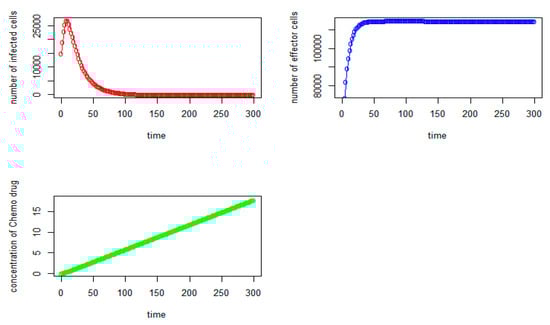
Figure 8.
Tumor virus-infected cells (red), The immune-effector cells (blue) and Concentration of Chemo drug (green) versus time (days) for the initial values: V = 15,000, I = 50,000, Q = 0).
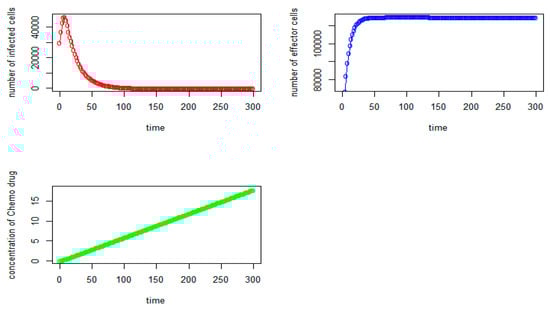
Figure 9.
Tumor virus-infected cells (red), immune-effector cells (blue), and concentration of chemo drug (green) versus time (days) for the initial values: V = 30,000, I = 50,000, Q = 0).
4. Conclusions
In this paper, we have formulated a mathematical model of the immune system with time-delay effects of the interactions between immune cells and tumor cells with autoimmune disease incorporating chemotherapy drug treatment, where the amount of drug injected to patients is kept constant using partial differential equations. The model can be used to determine the dynamic progression of tumor virus cells growth and observe the patterns of how the tumor cells spread in the body’s immune system subject to the time delays. It can be used to predict the spread of tumor cancer cells and when the tumor virus-free state can be reached as time progresses, as well as the number of body’s immune cells at any given time. From the numerical examples, we can observe that the initial number of tumor virus-infected cells and immune-effector cells that are needed to obtain the solutions of the delay partial differential equations do not influence the end results. Based on the obtained results above, one can extend this study to a more complicated model by considering a dynamic amount of chemotherapy drug injected, instead of a constant amount, to a patient based on the stage of the tumor cells as time progresses.
Funding
This research received no external funding.
Conflicts of Interest
The author declares no conflict of interest.
References
- Thompson, E. The immune system. J. Am. Med. Assoc. JAMA 2015, 313, 16. [Google Scholar] [CrossRef] [PubMed]
- CRI Staff. How Does the Immune System Work? 30 April 2019. Available online: https://www.cancerresearch.org/blog/april-2019/how-does-the-immune-system-work-cancer?gclid=CjwKCAjwsNiIBhBdEiwAJK4khgG7w-9Ugv3HMGc1VWZbRuhFBOfIPMW2Qo3Dv1-VH1HGvmJruZjwxxoC3HYQAvD_BwE (accessed on 15 May 2021).
- Guide to Your Immune System. 2020. Available online: https://www.webmd.com/cold-and-flu/ss/slideshow-immune-system (accessed on 20 May 2021).
- Immune System, Cleveland Clinic. 2021. Available online: https://my.clevelandclinic.org/health/articles/21196-immune-system (accessed on 10 May 2021).
- Newman, T. How the Immune System Works. Medical News Today. 11 January 2018. Available online: https://www.medicalnewstoday.com/articles/320101 (accessed on 20 May 2021).
- How Does the Immune System Work? 2020. Available online: https://www.ncbi.nlm.nih.gov/books/NBK279364/ (accessed on 20 May 2021).
- Ng, J.; Stovezky, Y.R.; Brenner, D.J.; Formenti, S.C.; Shuryak, I. Development of a model to estimate the association between delay in cancer treatment and local tumor control and risk of metastates. JAMA Netw. Open 2021, 4, e2034065. [Google Scholar] [CrossRef]
- Talkington, A.; Durrett, R. Estimating tumor growth rates in vivo. Bull. Math. Biol. 2015, 77, 1934–1954. [Google Scholar] [CrossRef]
- Vaghi, C.; Rodallec, A.; Fanciullino, R.; Ciccolini, J.; Mochel, J.P.; Mastri, M. Population modeling of tumor growth curves and the reduced Gompertz model improve prediction of the age of experimental tumors. PLoS Comput. Biol. 2020, 16, e1007178. Available online: https://journals.plos.org/ploscompbiol/article?id=10.1371/journal.pcbi.1007178 (accessed on 25 April 2021). [CrossRef]
- Yin, D.J.; Moes, A.R.; van Hasselt, J.G.C.; Swen, J.J.; Guchelaar, H.-J. A Review of Mathematical Models for Tumor Dynamics and Treatment Resistance Evolution of Solid Tumors. CPT Pharmacomet. Syst. Pharmacol. 2019, 8, 720–737. [Google Scholar] [CrossRef]
- Bekiros, S.; Kouloumpou, D. SBDiEM: A new mathematical model of infectious-disease dynamics. Chaos Solitons Fractals 2020, 136, 109828. [Google Scholar] [CrossRef] [PubMed]
- Rothan, H.A.; Byrareddy, S.N. The epidemiology and pathogenesis of coronavirus disease (COVID-19) outbreak. J. Autoimmun. 2020, 2020, 102433. [Google Scholar] [CrossRef]
- Jackson, T.L.; Byrne, H.M. A mathematical model to study the effects of drug resistance and vasculature on the response of solid tumors to chemotherapy. Math. Biosci. 2000, 164, 17–38. [Google Scholar] [CrossRef]
- Meacham, C.E.; Morrison, S.J. Tumour heterogeneity and cancer cell plasticity. Nature 2013, 501, 328–337. [Google Scholar] [CrossRef]
- Sun, X.; Bao, J.; Shaob, Y. Mathematical modeling of therapy-induced cancer drug resistance: Connecting cancer mechanisms to population survival rates. Sci. Rep. 2016, 6, 22498. [Google Scholar] [CrossRef]
- Taniguchi, K.; Okami, J.; Kodama, K.; Higashiyama, M.; Kato, K. Intratumor heterogeneity of epidermal growth factor receptor mutations in lung cancer and its correlation to the response to gefitinib. Cancer Sci. 2008, 99, 929–9354. [Google Scholar] [CrossRef] [PubMed]
- Al-Huniti, N.; Feng, Y.; Yu, J.; Lu, Z.; Nagase, M.; Zhou, D.; Sheng, J. Tumor growth dynamic modeling in oncology drug development and regulatory approval: Past, present, and future Opportunities. CPT Pharmacomet. Syst. Pharmacol. 2020, 9, 419–427. [Google Scholar] [CrossRef] [PubMed]
- Cai, Y.; Kang, Y.; Wang, W. A stochastic SIRS epidemic model with nonlinear incidence rate. Appl. Math. Comput. 2017, 305, 221–240. [Google Scholar] [CrossRef]
- Cai, Y.; Jiao, J.; Gui, Z.; Liu, Y.; Wang, W. Environmental variability in a stochastic epidemic model. Appl. Math. Comput. 2018, 329, 210–226. [Google Scholar] [CrossRef]
- Berryman, A.A. The orgins and evolution of predator-prey theory. J. Ecol. Soc. Am. 1992, 73, 1530–1535. [Google Scholar] [CrossRef]
- He, X.; Zheng, S. Protection zone in a diffusive predator-prey model with Beddington DeAngelis functional response. J. Math. Biol. 2016, 75, 239–257. [Google Scholar] [CrossRef]
- Huang, Y.; Shi, W.; Wei, C.; Zhang, S. A stochastic predator–prey model with Holling II increasing function in the predator. J. Biol. Dyn. 2021, 15, 1–18. [Google Scholar] [CrossRef]
- Jana, S.; Kar, T. Modeling and analysis of a prey-predator system with disease in the prey. Chaos Solitons Fractals 2013, 47, 42–53. [Google Scholar] [CrossRef]
- Kaur, G.; Ahmad, N. On study of immune response to tumor cells in prey-predator system. Int. Sch. Res. Not. 2014, 2014, 346597. [Google Scholar] [CrossRef]
- Bandyopadhyay, M.; Chattopadhyay, J. Ratio-dependent predator-prey model: Effect of environmental fluctuation and stability. Nonlinearity 2005, 18, 913–936. [Google Scholar] [CrossRef]
- Liu, Q.; Jiang, D.; Hayat, T.; Alsaedi, A. Dynamics of a stochastic predator–prey model with stage structure for predator and Holling type II functional response. J. Nonlinear Sci. 2018, 28, 1151–1187. [Google Scholar] [CrossRef]
- Bonate, P.L. Comprehensive overview of tumor growth modeling. In Proceedings of the 9th American Conference of Pharmacometrics (ACOP), San Diego, CA, USA, 7–11 October 2018. [Google Scholar]
- Singh, M.; Poonam, K. Qualitative analysis of a predator-prey model in the presence of additional food to predator and constant-yield predator harvesting. Univ. J. Appl. Math. Comput. 2019, 7, 20–34. [Google Scholar]
- Lestari, E.R.; Arifah, H. Dynamics of a mathematical model of cancer cells with chemotherapy. J. Phys. Conf. Ser. 2019, 1320, 12026. [Google Scholar] [CrossRef]
- Li, S.; Wang, X. Analysis of a stochastic predator–prey model with disease in the predator and Beddington–Deangelis functional response. Adv. Differ. Equ. 2015, 2015, 224. [Google Scholar] [CrossRef]
- Liming, X.C.; Li, M.; Guo, B. Stability analysis of an HIV/AIDS epidemics model with treatment. J. Comput. Appl. 2009, 229, 313–323. [Google Scholar]
- Wahyuda, C.N.; Lestari, D. Local stability of AIDS epidemic model through treatment and vertical transmission with time delay. J. Phys. Conf. Ser. 2016, 693, 12010. [Google Scholar]
- Alho, J.M. Forecasting life expectancy: A statistical look at model choice and use of auxiliary series. In Old and New Perspectives on Mortality Forecasting; Demographic Research Monographs, Bengtsson, T., Keilman, N., Eds.; Springer: Berlin/Heidelberg, Germany, 2019. [Google Scholar]
- Pham, H. Modeling U.S. mortality and risk-cost optimization on life expectancy. IEEE Trans. Reliab. 2011, 60, 125–133. [Google Scholar] [CrossRef]
- Derouich, M.; Boutayeb, A. An Avian influenzam mathematical model. Appl. Math. Sci. 2008, 2, 1749–1760. [Google Scholar]
- Mukhopadhyaya, B.; Bhattacharyya, R. Dynamics of a delay-diffusion prey-predator Model with disease in the prey. J. Appl. Math. Comput. 2005, 17, 361–377. [Google Scholar] [CrossRef]
- Aparico, J.P.; Chavez, C.C. Mathematical modelling of tuberculosis epidemics. Math. Biosci. Eng. 2009, 6, 209–237. [Google Scholar]
- Chavez, C.C.; Sony, B.J. Dynamical models of tuberculosis and their applications. Math. Biosci. Eng. 2004, 1, 361–404. [Google Scholar] [CrossRef] [PubMed]
- De Pillis, L.G.; Gu, W.; Fister, K.R.; Head, T.; Maples, K.; Murugan, A.; Neal, T.; Yoshida, K. Chemoterapy for tumors: An analysis of the dynamics and a study of quadratic and linear optimal control. Math. Biosci. 2006, 209, 292–315. [Google Scholar] [CrossRef] [PubMed]
- Kuznetsov, V.; Makalkin, I.; Taylor, M.; Perelson, A. Nonlinear dynamics of immunogenic tumors: Parameter estimation and global bifurcation analysis. Bull. Math. Biol. 1994, 56, 295–321. [Google Scholar] [CrossRef]
- Tsygvintsev, A.; Marino, S.; Kirschner, D.E. A Mathematical Model of Gene Therapy for The Treatment of Cancer. In Mathematical Models and Methods in Biomedicine; Springer: New York, NY, USA, 2012; pp. 357–373. [Google Scholar]
- Waziri, A.S.; Estomih, S.; Oluwole, D. Mathematical modelling of HIV/AIDS dynamic with treatment and vertical transmission. Appl. Math. 2012, 3, 77–89. [Google Scholar] [CrossRef]
- Wang, Y.; Kuang, C.; Ding, S.; Zhang, S. Stability and bifurcation of a stage-structured predator-prey model with both discete and distributed delays. Chaos Solitons Fractals 2013, 46, 19–27. [Google Scholar] [CrossRef]
- Kumar, S.; Chattopadh, S. A bioeconomic model of two equally dominated prey and one predator system. Mod. Appl. Sci. 2010, 4, 84–96. [Google Scholar] [CrossRef][Green Version]
- Liu, M. Dynamics of a stochastic regime-switching predator-prey model with modified Leslie–Gower Holling-type II schemes and prey harvesting. Nonlinear Dyn. 2019, 96, 417–442. [Google Scholar] [CrossRef]
- Liu, M.; Bai, C. Dynamics of a stochastic one-prey two-predator model with Lévy jumps. J. Comput. Appl. Math. 2016, 284, 308–321. [Google Scholar] [CrossRef]
- Liu, M.; Bai, C.; Deng, M.; Du, B. Analysis of stochastic two-prey one-predator model with Lévy jumps. Physica A 2016, 445, 176–188. [Google Scholar] [CrossRef]
- Tripathi, J.; Abbas, S.; Thakur, M. Local and global stability analysis of a two prey one predator model with help. Commun. Nonlinear Sci. 2014, 19, 3284–3297. [Google Scholar] [CrossRef]
- Pang, P.; Wang, M. Strategy and stationary pattern in a three-species predator–prey model. J. Differ. Equ. 2004, 200, 245–273. [Google Scholar] [CrossRef]
- Jiao, J.; Wang, R.; Chang, H.; Liu, X. Codimension bifurcation analysis of a modified Leslie–Gower predator-prey model with two delays. Int. J. Bifurcat. Chaos 2018, 28, 1850060. [Google Scholar] [CrossRef]
- Nie, L.; Peng, J.; Teng, Z.; Hu, L. Existence and stability of periodic solution of a Lotka–Volterra predator-prey model with state dependent impulsive effects. J. Comput. Appl. Math. 2009, 224, 544–555. [Google Scholar] [CrossRef]
- Tian, Y.; Sun, K.; Chen, L. Comment on existence and stability of periodic solution of a Lotka–Volterra predator–prey model with state dependent impulsive effects. J. Comput. Appl. Math. 2010, 234, 2916–2923. [Google Scholar] [CrossRef][Green Version]
- Law, G.R. What do epidemiologists mean by ‘population mixing? Pediatric Blood Cancer 2008, 51, 155–160. [Google Scholar] [CrossRef]
- Haque, M.; Zhen, J.; Ventrino, E. An eco-epidemiological predator-prey model with standard disease incidence. Math. Methods Appl. Sci. 2008, 35, 875–898. [Google Scholar] [CrossRef]
- Jiang, D. Analysis of a predator-prey model with disease in the prey. Int. J. Biomath. 2013, 6, 1350012. [Google Scholar]
- Naji, R.K.; Mustafa, A.N. The dynamics of an eco-epidemiological model with nonlinear incidence rate. J. Appl. Math. 2012, 11, 853–862. [Google Scholar] [CrossRef]
- Pal, P.; Haque, M.; Mandal, P. Dynamics of a predator–prey model with disease in the predator. Math. Methods Appl. Sci. 2013, 37, 2429–2450. [Google Scholar] [CrossRef]
- Xiao, Y.; Chen, L. Modeling and analysis of a predator–prey model with disease in the prey. Math. Biosci. 2001, 171, 59–82. [Google Scholar] [CrossRef]
- Xu, R.; Zhang, S. Modelling and analysis of a delayed predator–prey model with disease in the predator. Appl. Math. Comput. 2013, 224, 372–386. [Google Scholar] [CrossRef]
- Battegay, M. 2019-novel Coronavirus (2019-nCoV): Estimating the case fatality rate—A word of caution. Swiss Med. Wkly. 2020, 150, 506. [Google Scholar] [CrossRef] [PubMed]
- Chin, A.W.H.; Chu, J.T.S.; Perara, M.R.A.; Hui, K.P.Y.; Yen, H.-L.; Chan, M.C.W.; Paris, M.; Poon, L.L.M. Stability of SARS-CoV-2 in different environmental conditions. Lancet Mircobe 2020, 20, e145. [Google Scholar] [CrossRef]
- Kucharski, J. Early dynamics of transmission and control of COVID-19: A mathematical modelling study. Lancet Infect. Dis. 2020, 20, 553–558. [Google Scholar] [CrossRef]
- Pham, H. On estimating the number of deaths related to Covid-19. Mathematics 2000, 8, 655. [Google Scholar] [CrossRef]
- Pham, H. Estimating the COVID-19 death toll by considering the time-dependent effects of various pandemic restrictions. Mathematics 2020, 8, 1628. [Google Scholar] [CrossRef]
- Pham, H.; Pham, D.H. A novel generalized logistic dependent model to predict the presence of breast cancer based on biomarkers. Concurr. Comput. Pract. Exp. 2020, 32, 1. [Google Scholar] [CrossRef]
- Asamoah JK, K.; Jin, Z.; Sun, G.Q.; Seidu, B.; Yankson, E.; Abidemi, A.; Oduro, F.T.; Moore, S.E.; Okyere, E. Sensitivity assessment and optimal economic evaluation of a new COVID-19 compartmental epidemic model with control interventions. Chaos Solitons Fractals 2021, 146, 110885. [Google Scholar] [CrossRef]
- Pham, H. A dynamic model of multiple time-delay interactions between the virus-infected cells and body’s immune system with autoimmune diseases. Axioms 2021, 10, 216. [Google Scholar] [CrossRef]
Publisher’s Note: MDPI stays neutral with regard to jurisdictional claims in published maps and institutional affiliations. |
© 2022 by the author. Licensee MDPI, Basel, Switzerland. This article is an open access article distributed under the terms and conditions of the Creative Commons Attribution (CC BY) license (https://creativecommons.org/licenses/by/4.0/).