Reconstructing Dynamic 3D Models with Small Data by Integrating Position-Based Dynamics and PDE-Based Modelling

Abstract

Simulation with position-based dynamics is very popular due to its high efficiency. However, it has the weaknesses of lacking details when too few vertices are involved in simulation and inefficiency when too many vertices are used for simulation. To tackle this problem, in this paper, we propose a new method of reconstructing dynamic 3D models with small data. The core elements of the proposed approach are a curve-represented geometric model and a physics-based mathematical model defined by dynamic partial differential equations. We first use the simulation method of position-based dynamics to generate a group of keyframe poses, which are used to create the deformation animation of a 3D model. Then, wireframe curves are extracted from skin deformation shapes of the 3D model at different keyframe poses. A physics-based mathematical model defined by dynamic partial differential equations is proposed. Its closed-form solution is obtained to represent the extracted curves, which are used to reconstruct the deformation models at different keyframe poses. Experimental examples and comparisons made in this paper indicate that the proposed method of reconstructing dynamic 3D models can greatly reduce data size while keeping good details.

1. Introduction

With the rapid development of the gaming industry, the demand for a high degree of accuracy in game scenes has led to the increasing need to quickly animate more detailed 3D models. In order to create efficient and realistic shape changes, various shape deformation methods have been proposed, which could be roughly divided into geometric, data-driven, and physics-based methods.

Geometric methods [1,2,3,4,5] are the most efficient but less capable of generating realistic shape deformation since they do not consider any physics of shape changes. Data-driven techniques [6,7,8,9,10] use known example models to create new deformation results. This type of method can generate highly realistic deformation results with sufficient high-quality examples. Similar to geometric methods, data-driven methods do not take the physics of shape changes into account. Therefore, they require enough shape examples to achieve authenticity. Generating enough shape examples is a main weakness of data-driven methods. How to reduce the number of example shapes without losing realism is a primary issue of data-driven methods. In contrast, physics-based approaches [11,12,13,14] consider the underlying physics of object movements and deformations to create more realistic deformations. Unfortunately, physics-based approaches rely on heavy numerical calculations and are not ideal in many applications requiring high computing performance.

To achieve the balance between efficiency and realism, position-based dynamics (PBD) [15,16,17] is introduced. With a relatively high deformation performance, PBD tackles the problem of the numerical calculation needed for physics-based techniques. Its high simulation performance makes PBD-based methods popular in computer games and interactive applications. However, the simulation with PBD is based on discrete vertices of polygon models and influenced by the number of vertices involved in the simulation. When too few vertices are involved in the simulation, the results are not detailed, causing less realistic deformations. On the contrary, too many vertices involved in the simulation cause a significant reduction in the calculation efficiency.

As shown in Figure 1, the dog model in (a) with 502 vertices and 1000 faces is very rough with no details. The corresponding dog models become more detailed as the vertices and faces increase further from (a) to (d).

Table 1. Computational time (CPU) of position-based simulation for a dog model with different faces.

Model\TET	100,000	20,000	4000	1000
100,000	243.43 s	76.74 s	12.15 s	3.51 s
20,000	/	75.32 s	13.19 s	3.34 s
4000	/	/	12.62 s	3.25 s
1000	/	/	/	3.15 s

shows how different faces of the same polygon model affect the CPU time of PBD simulations. In order to carry out PBD simulations, a polygon surface model must be first converted into a corresponding tetrahedron model, which is used in keyframes to compute its deformation results by the PBD software library [18]. In Table 1, we listed the face number of an original dog model in the first column and the face number of the corresponding tetrahedron model in the first row. In order to achieve different simulation accuracies, the converted tetrahedron model can have different resolutions, i.e., different face numbers. In this paper, we only consider the cases where the face number of the converted tetrahedron model is not more than the face number of the original model. Since new positions of model vertices are determined by collision and deformation of the corresponding tetrahedron model, different combinations of original and tetrahedron models will cause different results and time consumption. When the polygon dog model and its tetrahedron version have 1000 faces, the simulation takes 3.15 s to complete. As the faces of the polygon dog model and its tetrahedron version increase, the computational time quickly increases. When the faces of the polygon dog model and its tetrahedron version increase to 100,000, the simulation time increases to 243.43 s.

The above discussions indicate that discrete representations of 3D models cause the problem of either poor details or low computational efficiency. How to further improve PBD to achieve both good details and high computational efficiency is an unsolved topic.

Continuous representations of 3D models can noticeably reduce the design variables of discrete representations. Introducing continuous representations would tackle the above problem. There are several methods that can be used to reconstruct discrete 3D models with continuous representations. These reconstruction methods include using patch-based modelling approaches such as Bézier, B-spline, Non-Uniform Rational B-Splines (NURBS), ordinary differential equation (ODE), and partial differential equation (PDE). Among them, Bézier-, B-spline-, and NURBS-based reconstruction has been developed in [19,20,21,22,23].

ODE-based modelling [24,25,26] uses the solution of a vector-valued ODE to create a 3D curve, and then sweeps the 3D curve along two boundary curves subject to continuous requirements to create 3D models. Since the solution to ODEs may involve complicated mathematical functions such as sine and cosine functions and/or their combinations with other mathematical functions, a single ODE patch has the potential to create a more complicated shape than polygon modelling and a single Bézier, B-spline, and NURBS patch with the same number of design variables. A simple example is given by the different mathematical representations of a circle. When using sine and cosine functions to represent the circle, only one design variable, i.e., the radius of the circle, is involved. Clearly, polygon modelling, Bézier, B-spline, and NURBS cannot use one design variable to create the circle.

Similar to ODE-based modelling, PDE-based modelling [27,28,29,30,31] uses the solution of a vector-valued PDE subjected to boundary constraints to create 3D models. It was reported in [32] that for an original femur polygon mesh with a size of 3.2 MB, the NURBS approximation reduces the size to 0.55 MB, and the analytical PDE approximation reduces the size to 0.26 MB, indicating that analytical PDE-based modelling can significantly reduce design variables in comparison with polygon modelling and other patch-based modelling techniques.

PDE-based modelling, without considering the effects of acceleration and velocity, is called static PDE-based modelling. It has been well-investigated. For objects in motion, the effects of acceleration and velocity are considered in physics-based modelling. When PDE-based modelling is used to deal with these situations, the effects of acceleration and velocity are involved in PDEs, and the corresponding PDE-based modelling is called dynamic PDE-based modelling. Although much work has investigated PDE-based modelling, few of them are about dynamic PDE-based modelling. We have not found any work which integrates dynamic PDEs with PBD to reconstruct dynamic 3D models obtained from PBD simulations. Apart from the advantage of the dynamic PDE-based modelling in reducing the number of design variables, 3D models reconstructed from dynamic PDE-based modelling are time-dependent. By setting the time variable involved in mathematical expressions defining dynamic 3D models to different values, some keyframes simulated by PBD can be replaced by those generated with the corresponding dynamic PDE-based modelling. In doing so, some PBD simulation calculations can be avoided and PBD simulation efficiency can be improved.

Motivated by the above discussions, this paper will combine the fourth-order ordinary differential equation, describing the bending deformations of elastic beams, with Newton’s second law of motion, which describes the underlying physics of object movements, to achieve physics-based dynamic simulation while avoiding heavy numerical calculations of physics-based simulations.

The remaining parts of this paper will be organised as follows. Related work will be reviewed in Section 2. Deformation simulation with PBD will be introduced in Section 3. The mathematical model and its closed-form solution will be investigated in Section 4. Experimental examples and comparisons will be made in Section 5. Conclusions and future work will be discussed in Section 6.

2. Related Work

The work carried out in this paper is related to shape deformations and parametric surface-based 3D reconstruction, and continuous ODE and PDE based modelling. In this section, we briefly review the existing work in these areas.

2.1. Shape Deformations

Shape deformations can be achieved through manual creation or automatic generation. The aim of this paper is to integrate PBD and PDE, and PBD automatically generates shape deformations. Therefore, in this subsection, we review automatic shape deformation generation methods, which can be divided into geometric, data-driven and physics-based ones.

• Geometric shape deformations relate skin shape changes to the underlying skeleton movements. Among various geometric shape deformation methods, Linear Blend Skinning [1] is most popular due to its efficiency and simplicity. Unfortunately, it has the artefacts of collapsing joints and candy-wrapper effects, etc. In order to overcome these artefacts, Dual Quaternion blending [2] was proposed. Although it eliminates the artefacts of collapsing joints and candy-wrapper effects, it causes a new problem called joint-bulging artefact. The Delta Mush algorithm [3] treats skinning as a problem of smoothing the low-frequency geometry while preserving detail to avoid manual weight painting, which is required in existing geometric skinning methods. Since the Delta Mush algorithm involves heavy iterative calculations, the Direct Delta Mush algorithm [4] was proposed to improve the efficiency and control of the Delta Mush algorithm at the cost of high storage requirements. In order to tackle this problem, a compression method was introduced into the Direct Delta Mush algorithm in [5] to reduce its storage and run-time computing costs.

Geometric shape deformation methods are simple, efficient, easily controllable, and suitable for the applications requiring high performance. However, they are less capable of creating realistic shape changes.

• Data-driven shape deformations are proposed to improve the realism of shape changes. They treat the problem as a general data regression that learns the relationship between shape changes and skeleton movements from example shapes. Pose Space Deformation (PSD) [6] improves shape interpolation by representing shape changes as mappings from a pose space defined by a skeleton or a more abstract system of parameters to displacements. PSD requires a large amount of memory and is not suitable for use in interactive systems. This problem was tackled in [7] by fitting the parameters of a deformation model to best approximate the example data. The method proposed in [8] automatically extracts linear blending skinning by learning from a set of example poses. In recent years, machine learning has been introduced into data-driven methods. In [9], mesh deformations were split into linear and non-linear ones. The transformations of the skeleton underlying the mesh were used to determine the linear deformations, and deep learning was used to approximate remaining non-linear deformations. RigNet [10] predicted a skeleton to match an input 3D articulated character model and estimated surface skin weights by learning example data in a dataset.

Data-driven methods can create realistic shape changes when example shapes are sufficient and high-quality example shapes are obtained. The main weakness of data-driven methods is the preparation of many high-quality example shapes.

• Physics-based shape deformations are introduced to tackle the problem of geometric methods in creating less realistic shapes and address the weakness of data-driven methods in requiring enough high-quality example shapes. Various physics-based shape deformation models have been developed as reviewed in [11]. Among these models, the three most important physics-based deformable models are mass-spring systems, the finite element method (FEM), and finite volume method. In [12], a mass-spring system of a facial muscle model was developed. For the simulation of elastic and elastoplastic fracturing materials, FEM is more effective and can generate more realistic results [13]. The finite volume method [14] employs a divergence-free vector field, representing solid shape deformations without losing self-interactions or features.

Due to the consideration of underlying physics, physics-based methods can create more realistic shape changes than geometric methods. However, due to the expensive cost involved in numerical calculations of physics-based methods, various physics-based approaches are mainly applied in movies and other applications requiring good realism. Since computer games require both high efficiency and good realism, physics-based methods are not ideal for computer games.

• Position-based dynamics makes a good compromise between realism and efficiency. It is initially proposed for solid simulation, such as cloth simulation [15]. Since bending constraints are determined by the dihedral angle rather than edge lengths, they and stretching constraints are separated into two independent parameters. Müller et al. have used this method to generate robust cloth simulation with high controllability. Macklin et al. have presented an alternative approach to simulate fluids in the PBD framework [16] by modelling the fluids as a particle system. Each particle is constrained by a minimum distance from others. Compared with force-based fluids simulation, the method of position-based fluids uses a larger time step with a comparable result, which significantly reduces the computation cost. Besides the particle-based models, the position-based method has also been applied in rigid body simulation by solving constraints between rigid bodies [17].

This paper will take advantage of position-based dynamics in making a good compromise between realism and efficiency but tackle its weakness caused by discrete representations. Our approach is to obtain detailed deformation shapes at a few keyframes with position-based dynamics, use our proposed dynamic reconstruction to convert the discrete representations of the detailed deformation shapes into continuous representations, and create more deformation shapes with the same details from the continuous representations to reduce the number of design variables and raise simulation efficiency of position-base dynamics.

2.2. Parametric Surfaces-Based Reconstruction

In existing research studies, polygonal, implicit, and parametric surfaces have been used in 3D reconstruction. Here we review existing works on parametric surface-based reconstruction techniques, including Bézier, B-spline, and NURBS surfaces, which can be more easily represented with analytical mathematical expressions.

Bézier surfaces were used to reconstruct the 3D model of a broken blade in [19]. Bézier and B-splines techniques were introduced in [20,21,22]. Bézier surfaces have the weakness that they cannot be modified locally, and the local modification of control points will affect the shape of the entirety of all the Bézier surfaces. Besides, the polynomial order of Bézier surfaces is related to the number of vertices, which makes it not flexible to manipulate the whole surface, and as larger vertices number leads to higher polynomial order, the polygon control over the shape of the curve will be significantly weakened. Hence, to overcome the weakness of the Bezier surface technique, the B-splines surface method was developed to provide local modification of the surface. In addition, B-splines have the advantages that the polynomial degree of a B-spline can be independent of the number of control points. When the degree is lower, the B-spline curve follows the control polyline more closely.

However, both Bézier and B-splines have some limitations, such as the incapability in accurately representing conics and complicated shapes, whilst NURBS do not have these limitations, as discussed in [21,23]. They have become an industry standard and been included in various geometric modelling and computer graphics software packages due to their generality, the same excellent properties as B-splines, and incorporation in international standards.

Bézier, B-spline, and NURBS functions are constructed using polynomials. In contrast, the solutions to ODEs and PDEs may contain complicated mathematical functions, which will be introduced in Section 2.3. Due to this reason, a single Bézier, B-spline, and NURBS patch may not be as capable as a single ODE or PDE patch in creating a complicated shape.

2.3. ODE and PDE Based Modelling

Since ODEs and PDEs are widely used in science and engineering to describe underlying physics, ODE- and PDE-based geometric modelling is physics-based. Like Bézier, B-spline, and NURBS surfaces, which have been used in 3D reconstruction, ODE and PDE surfaces can also be used in 3D reconstruction. Here we briefly review some work in ODE- and PDE-based modelling.

• ODE-based modelling sweeps a curve defined by the solution to a vector-valued ODE along two boundary curves subject to continuity constraints on boundary curves to create an ODE surface. Various ODE-based modelling methods have been developed. For example, ODE-based sweeping surfaces were proposed in [24], ODE-based surface blending was investigated in [25], and ODE-based skin deformations were discussed in [26]. Since solving an ODE is easier than solving a PDE, ODE-based modelling is easier than PDE-based modelling. One weakness of ODE-based modelling is the difficulty of manipulating ODE sweeping surfaces since the manipulation is carried out on curves.

• PDE-based modelling uses the solution to a vector-valued PDE subject to given boundary constraints to define a PDE surface. PDE-based modelling has received a lot of research attention. Here we briefly review some work on PDE-based modelling using continuous PDE surfaces defined with analytical solutions to PDEs. PDE-based modelling of free form surfaces was pioneered in [27], where a vector-valued fourth-order PDE with one shape control parameter was used. Then it was used to develop the technique of interactive design [28] and achieve PDE surface-based reconstruction [29]. The current state in PDE-based modelling is analytical PDE-based skin deformation [30] and real-time PDE surface manipulation [31].

Although there has been much work on PDE-based modelling using continuous PDE surfaces and PDE surface-based reconstruction has also been investigated, few research studies investigate dynamic PDE-based modelling. To the best of our knowledge, we are unaware of any work that integrates dynamic PDE-based modelling and PBD simulation to reconstruct dynamic 3D models.

In this paper, a physics-based dynamic model represented with PDE will be developed from the governing equation for the bending deformations of elastic beams and Newton’s second law for object motion. The separation of variables will be used to transform a PDE into two ODEs. The closed-form solutions to the two ODEs will be obtained to achieve the dynamic reconstruction of deformed 3D models at different keyframes.

3. Deformation Simulation with Position-Based Dynamics

Position based dynamics (PBD) methods were developed for specific use in interactive environments. Unlike the traditional simulation methods for dynamic scenes using the force to represent the momentum change and calculate the position of each vertex, position-based approaches directly focus on the position alteration, omitting the velocity and acceleration. Compared with force-driven techniques, PBD has advantages of simplicity, efficiency, and robustness [33]. Due to these advantages, they have become very popular in computer graphics and the gaming industry in recent years.

3.1. The Development of PBD

Due to its high efficiency, position-based dynamics has been widely applied in the graphics field, recently including computer games. Müller et al. first introduced Position-Based Dynamics as a generalised framework capable of solving a large variety of constraints [15]. They demonstrated PBD applications on many types of deformable solids. Unlike the physics-based skin deformation methods, these methods use the solution of a quasi-static problem to calculate each timestep’s position change directly. When using an explicit time integration scheme, it avoids the issues of force-based simulation models like overshooting. They are more appropriate when computing object interaction due to their versatility, robustness, controllability, and efficiency.

Nevertheless, as they do not satisfy underlying physics laws, position-based approaches are only plausible in vision and have problems such as the failure in converging to a particular solution. To speed up the convergence brought by the Gauss–Seidel-type manner of the PBD solver in early work, a multi-grid-based strategy was used to process general non-linear constraints [34], which makes the simulation process more suitable for interactive applications such as computer games. To obtain a more complex physical phenomenon, Bender et al. proposed a continuum-based formulation and regarded strain-energy as a constraint function for the PBD solver [35]. Besides, the previous PBD methods suffer from a longstanding problem: constraints can become arbitrarily stiff because of the iteration count and time step. In order to address this problem, Macklin et al. introduced the XPBD method, which uses a new constraint formulation and the Lagrange multiplier for solving constraints in a time step and iteration count independent manner [36]. A thorough overview of various PBD methods has been made in [33]. Volume conservation among all collision constraints plays a significant role in the dynamic simulation of deformable bodies, especially for the simulation of tetrahedral meshes, such as the horse model used in this paper where a constraint to conserve the volume of a single tetrahedron has to be considered. It has been addressed in [37,38].

3.2. PBD Algorithm Overview

The overview of the PBD algorithm in [15] could be roughly considered as a loop with the following four steps for each timestep $\Delta t$:

• Get the initial attributes of vertices of the mesh, including the initial coordinates $x^0$, velocity $v^0$, and weight $w=1/ m$($m$ denotes the mass of the vertex);
• Each vertex will update its velocity $v$ as well as its predicted position $p$ by the external force ${\mathit{f}}_{ext}$ according to the following formula:

  $$\begin{array}{c}v=v^0+\Delta t{\mathit{f}}_{ext}w\\ p=x^0+\Delta tv\end{array}$$
• After the predicted position $p$ has been gained, add constraints, including collisions, volume conservation, cloth balloons, and so on. The position $p$ will be directly modified to $p^{\prime }$ with a group of iterations:

  $$p^{\prime }=projectConstraints\left(C_1, \dots , C_M,p_1,\dots ,p_N\right)$$

  where $M$ stands for the number of constraints and $N$ denotes the solver iteration number;
• Finally, the position change $\Delta p=p^{\prime }-x^0$ will be reused to calculate the attributes $v^1$ and $x^1$:

  $$\begin{array}{c}{v}^1=\Delta p / \Delta t\\ x^1=p^{\prime }\end{array}$$

  where $x^1$ and $v^1$ will be used as the initial information of the vertices in the loop of the next timestep.

3.3. Our PBD Simulation Experiment

The software library “PositionBasedDynamics” was developed from position-based dynamics by Bender et al. for the physically-based simulation of rigid bodies, deformable solids, and fluids. It is available from the link given in [18]. In this subsection, we use it to obtain the PBD simulation results of deforming a horse model on an Intel i7 6700 CPU with a clock rate of 3.4 GHz for use in the following Section 5 by our proposed approach.

After checking all examples in the package, we finally chose the SceneLoaderDemo as our simulation environment as it allows us to use custom models with plausible deformation results. We first use tetGenerator to create the tetrahedral data of a curve-based horse model. Then, we input both the horse model and its corresponding tetrahedral files into the program to generate 100 sequential keyframes and obtain the deformation animation.

Figure 2 shows the results of the PBD simulation. As could be seen, the neck part has been significantly deformed with torsion and stretching. In what follows, we will propose a PDE-based modelling algorithm to reduce design variables in Section 4 and Section 5 below. Besides, we will extend the functionality of the proposed PDE-based modelling algorithm in reducing design variables to the replacement of some PBD simulation calculations in our future work. With the improved algorithm, the computational time of PBD simulation will be shortened.

4. Mathematical Model and Closed-Form Solution

In the field of geometric modelling and computer animation, physics-based methods are developed to improve simulation realism. As stated in [39,40], physics-based modelling has improved the realism of animated objects and physics-based models provide realistic 3D geometry of the bones and muscles.

Newton’s second law has been used to develop physics-based dynamic simulations for computer animation, etc., in existing research studies. Although Newton’s second law actually applies only to particles [41], it was also used to describe shape changes of 3D models such as in [42,43] to describe deformations of 3D facial models, in [44] to simulate soft tissue deformation for virtual surgery applications, in [45] to describe dynamics of facial tissues, and in [46] to describe dynamic deformations of cloth motion. In this paper, Newton’s second law will also be introduced to develop a physics-based method.

A surface can be generated by sweeping a curve. Similar to existing methods that use Newton’s second law to simulate surface deformations, Newton’s second law can be used to describe curve deformations. Newton’s second law only applies to particles. When discretizing a curve into points, each point is treated as a particle. When using Newton’s second law to simulate movements of these points, each of the points moves independently. This does not conform with the fact that the points defining a curve cannot move independently. Curve deformations are similar to beam deformations. Therefore, introducing the governing equation of beam deformations into Newton’s second law can tackle the problem that the points defining a curve move independently when simulating their movements with Newton’s second law only.

For physics-based modelling, achieving good realism requires accurate models, which involves heavy numerical calculations leading to low efficiency. In order to obtain a good balance between realism and efficiency, simplified physics-based models are usually used in computer animation and computer games, etc. For example, soft tissues are simplified as an isotropic and linear elastic material in [47] for finite element simulations of anatomy- and physics-based facial animation, although they have anisotropic, nonhomogeneous, and non-linear elastic mechanical behaviours. With the same treatment, we will simplify deformations of 3D models as isotropic and linear elastic and use Young’s modulus to describe their mechanical properties in this paper.

Based on the above discussions, we integrate Newton’s second law of motion and the governing equation for bending deformations of elastic beams to develop a new mathematical model, obtain the closed-form solution of the mathematical model, and combine the closed-form solution with position-based dynamics to develop a dynamic reconstruction method for reconstructing dynamic 3D models with small data.

As discussed above, Newton’s second law of motion has been applied in computer animation, etc., to develop physics-based dynamic simulations [42]. It describes the relationship between the product of the mass and acceleration of an object and the external forces acting on the object, i.e.,

$$ma=f$$

(1)

When considering the bending deformation of an elastic beam, the governing equation is [48]:

$$EI\frac{d^{4}w}{d{x}^4}=f$$

(2)

where $EI$ denotes the flexural rigidity and $w\left(x\right)$ describes the deflection of the beam.

Combining (1) and (2), we have:

$$ma=EI\frac{d^{4}w}{d{x}^4}$$

(3)

As derived in Appendix A, the mathematical model for reconstructing dynamic 3D models can be obtained from Equation (3) and has the following form:

$$m\frac{{\partial }^{2}w}{\partial t^2}=D\frac{{\partial }^{4}w}{\partial u^4} \left(w=x,y,z\right)$$

(4)

In order to solve the above PDE, we use the method of separation of variables [49] to solve Equation (4). As derived in Appendix B, the closed-form solutions to Equation (4) can be written as the following four forms:

For the case $c_{w0}/m>0$ and $c_{w0}/D>0$:

$$\begin{array}{cc}\hfill w\left(u,t\right) =c_{w1}{e}^{m_{w0}t}& e^{D_{w0}u}+c_{w2}{e}^{m_{w0}t}{e}^{-D_{w0}u}+c_{w3}{e}^{m_{w0}t}cos{D}_{w0}u\hfill \\ & +c_{w4}{e}^{m_{w0}t}sin{D}_{w0}u+c_{w5}{e}^{-m_{w0}t}{e}^{D_{w0}u}+c_{w6}{e}^{-m_{w0}t}{e}^{-D_{w0}u}\hfill \\ & +c_{w7}{e}^{-m_{w0}t}cos{D}_{w0}u+c_{w8}{e}^{-m_{w0}t}sin{D}_{w0}u\hfill \\ & \left(w=x,y,z\right)\end{array}$$

(5)

For the case $c_{w0}/m>0$ and $c_{w0}/D<0$:

$$\begin{array}{cc}\hfill w\left(u,t\right) =c_{w1}{e}^{m_{w0}t}& e^{D_{w1}u}cos{D}_{w1}u+c_{w2}{e}^{m_{w0}t}{e}^{D_{w1}u}sin{D}_{w1}u\hfill \\ & +c_{w3}{e}^{m_{w0}t}{e}^{-D_{w1}u}cos{D}_{w1}u+c_{w4}{e}^{m_{w0}t}{e}^{-D_{w1}u}sin{D}_{w1}u\hfill \\ & +c_{w5}{e}^{-m_{w0}t}{e}^{D_{w1}u}cos{D}_{w1}u+c_{w6}{e}^{-m_{w0}t}{e}^{D_{w1}u}sin{D}_{w1}u\hfill \\ & +c_{w7}{e}^{-m_{w0}t}{e}^{-D_{w1}u}cos{D}_{w1}u+c_{w8}{e}^{-m_{w0}t}{e}^{-D_{w1}u}sin{D}_{w1}u\hfill \\ & \left(w=x,y,z\right)\end{array}$$

(6)

For the case $c_{w0}/m<0$ and $c_{w0}/D>0$:

$$\begin{array}{cc}\hfill w\left(u,t\right) =c_{w1}cos& \left(m_{w0}t\right)e^{D_{w0}u}+c_{w2}cos(m_{w0}t)e^{-D_{w0}u}\hfill \\ & +c_{w3}cos(m_{w0}t)cos(D_{w0}u)+c_{w4}cos\left(m_{w0}t\right)sin\left(D_{w0}u\right)\hfill \\ & +c_{w5}sin(m_{w0}t)e^{D_{w0}u}+c_{w6}sin(m_{w0}t)e^{-D_{w0}u}\hfill \\ & +c_{w7}sin\left(m_{w0}t\right)cos\left(D_{w0}u\right)+c_{w8}sin(m_{w0}t)sin(D_{w0}u)\hfill \\ & \left(w=x,y,z\right)\end{array}$$

(7)

For the case $c_{w0}/m<0$ and $c_{w0}/D<0$:

$$\begin{array}{cc}\hfill w\left(u,t\right) =c_{w1}cos& \left(m_{w0}t\right)e^{D_{w1}u}cos{D}_{w1}u+c_{w2}cos(m_{w0}t)e^{D_{w1}u}sin{D}_{w1}u\hfill \\ & +c_{w3}cos(m_{w0}t)e^{-D_{w1}u}cos{D}_{w1}u\hfill \\ & +c_{w4}cos\left(m_{w0}t\right)e^{-D_{w1}u}sin\left(D_{w1}u\right)\hfill \\ & +c_{w5}sin(m_{w0}t)e^{D_{w1}u}cos{D}_{w1}u\hfill \\ & +c_{w6}sin(m_{w0}t)e^{D_{w1}u}sin{D}_{w1}u\hfill \\ & +c_{w7}sin\left(m_{w0}t\right)e^{-D_{w1}u}cos\left(D_{w1}u\right)\hfill \\ & +c_{w8}sin(m_{w0}t)e^{-D_{w1}u}sin\left(D_{w1}u\right)\hfill \\ & \left(w=x,y,z\right)\end{array}$$

(8)

All the four Equations (5)–(8) can be used to reconstruct dynamic 3D models. In order to reconstruct dynamic 3D models using one of the four Equations (5)–(8), we first extract curves from the 3D models at the undeformed position called the first keyframe ($j=0$), and different deformation positions called $j\mathrm{th}$ ($1<j\le J$) keyframe. For each of the extracted curves, we find the minimum values $x_{min}$, $y_{min}$, and $z_{min}$ and maximum values $x_{max}$, $y_{max}$, and $z_{max}$ of the $x$, $y$, and $z$ components for all the $N+1$ points on the curve with the following equations:

$$\begin{array}{c}{w}_{min}=min\left\{\begin{array}{ccccc}{w}_0& w_1& \cdots & w_{N-1}& w_N\end{array}\right\}\\ w_{max}=max\left\{\begin{array}{ccccc}{w}_0& w_1& \cdots & w_{N-1}& w_N\end{array}\right\}\\ \left(w=x,y,z\right)\end{array}$$

(9)

Having obtained the minimum values $x_{min}$, $y_{min}$, and $z_{min}$ and maximum values $x_{max}$, $y_{max}$, and $z_{max}$ of the $x$, $y$, and $z$ components for all the $N+1$ points on the curve, we use the following equation to obtain the parametric values of the $n\mathrm{th}$ point on the curve:

$$\begin{array}{c}{u}_n=\frac{w_n-w_{min}}{w_{max}-w_{min}}\\ \left(w=x,y,z;n=0, 1, 2, \dots , N\right)\end{array}$$

(10)

When Equations (5)–(8) are used to reconstruct more than one curve, each curve to be reconstructed has its own parametric values of $u_n$ according to Equation (10), which may be different from each other. In Equations (5)–(8), $u_n$ must be the same value at the corresponding points of different curves to be reconstructed. In such a case, an average value of $u_n$ at the corresponding points of different curves is used in Equations (5)–(8).

If we use one of the four Equations (5)–(8) to reconstruct the dynamic models at $J$ keyframes, the time variable $t$ takes the value $t_j=j/J$ where $J$ is the total number of keyframes.

At the $n\mathrm{th}$ point of the $j\mathrm{th}$ keyframe, the position components of the point are $w_{j,n}$ obtained from the position-based dynamics. The position components calculated with one of Equations (5)–(8) are $w\left(u_n,t_j\right)$. If the dynamic models are accurately reconstructed, we have $w\left(u_n,t_j\right)=w_{j,n}$. If the dynamic models are not accurately reconstructed, we minimise the squared error sum between $w\left(u_n,t_j\right)$ and $w_{j,n}$ for all the $N+1$ points on the $J+1$ keyframes, i.e., minimise.

$$\begin{array}{c}{E}_w={\displaystyle \sum _{j=0}^J}{\displaystyle \sum _{n=0}^N}{\left[w\left(u_n,t_j\right)-w_{j,n}\right]}^2\\ \left(w=x,y,z\right)\end{array}$$

(11)

In what follows, we take Equation (5) as an example to demonstrate how to reconstruct dynamic 3D models.

Substituting Equation (3) into Equation (11), we obtain the squared error sum:

$$\begin{array}{cc}\hfill E_w={\displaystyle \sum _{j=0}^J}{\displaystyle \sum _{n=0}^N}& [c_{w1}{e}^{m_{w0}{t}_j}{e}^{D_{w0}{u}_n}+c_{w2}{e}^{m_{w0}{t}_j}{e}^{-D_{w0}{u}_n}+c_{w3}{e}^{m_{w0}{t}_j}cos{D}_{w0}{u}_n\hfill \\ & +c_{w4}{e}^{m_{w0}{t}_j}sin{D}_{w0}{u}_n+c_{w5}{e}^{-m_{w0}{t}_j}{e}^{D_{w0}{u}_n}+c_{w6}{e}^{-m_{w0}{t}_j}{e}^{-D_{w0}{u}_n}\hfill \\ & +c_{w7}{e}^{-m_{w0}{t}_j}cos{D}_{w0}{u}_n+c_{w8}{e}^{-m_{w0}{t}_j}sin{D}_{w0}{u}_n-w_{j,n}{]}^2\hfill \\ & \left(w=x,y,z\right)\end{array}$$

(12)

In the above equation, $c_{wi}\left(i=1,2,\dots ,8\right)$ are unknown constants, which can be optimised to minimise the squared error sum. To do this, we use the least squares method, which leads to the following equation:

$$\begin{array}{c}\frac{\partial E_w}{\partial c_{wi}}=0 \left(i=1, 2,\dots , 8\right)\\ \left(w=x,y,z\right)\end{array}$$

(13)

If we let,

$$\begin{array}{cc}\hfill f_w=[c_{w1}{e}^{m_{w0}{t}_j}& e^{D_{w0}{u}_n}+c_{w2}{e}^{m_{w0}{t}_j}{e}^{-D_{w0}{u}_n}+c_{w3}{e}^{m_{w0}{t}_j}cos{D}_{w0}{u}_n\hfill \\ & +c_{w4}{e}^{m_{w0}{t}_j}sin{D}_{w0}{u}_n+c_{w5}{e}^{-m_{w0}{t}_j}{e}^{D_{w0}{u}_n}\hfill \\ & +c_{w6}{e}^{-m_{w0}{t}_j}{e}^{-D_{w0}{u}_n}+c_{w7}{e}^{-m_{w0}{t}_j}cos{D}_{w0}{u}_n\hfill \\ & +c_{w8}{e}^{-m_{w0}{t}_j}sin{D}_{w0}{u}_n-w_{j,n}]\hfill \\ & \left(w=x,y,z\right)\end{array}$$

(14)

Equation (12) becomes:

$$\begin{array}{c}{E}_w={\displaystyle \sum _{j=0}^J}{\displaystyle \sum _{n=0}^N}{\left(f_w\right)}^2\\ \left(w=x,y,z\right)\end{array}$$

(15)

and Equation (13) is changed into:

$$\begin{array}{c}\frac{\partial E}{\partial c_{wi}}=2{\displaystyle \sum _{j=0}^J}{\displaystyle \sum _{n=0}^N}{f}_w\frac{\partial f_w}{\partial c_{wi}}=0 \left(i=1, 2,\dots , 8\right)\\ \left(w=x,y,z\right)\end{array}$$

(16)

Equation (16) consists of eight linear equations, which can be solved to determine the eight unknown constants $c_{wi}$ $\left(i=1, 2,\dots , 8\right)$. Substituting the obtained eight unknown constants $c_{wi}$ $\left(i=1, 2,\dots , 8\right)$ into Equation (5), Equation (5) becomes the mathematical expressions of the reconstructed curves at the ($J+1$) keyframes. All the curves of 3D models described by Equation (5) define the reconstructed 3D models.

As discussed in Section 2, Bézier, B-splines, and NURBS surfaces are frequently used to reconstruct the 3D models that do not change their positions and shapes with time. In this paper, such a type of reconstruction is called static reconstruction. In the following section, we compare our proposed dynamic reconstruction with Bézier and B-spline static reconstruction.

The mathematical equation of Bézier curves can be written as [50]:

$$w\left(u\right)={\sum }_{i=0}^k\frac{k!}{i!\left(k-i\right)!}{u}^i{\left(1-u\right)}^{k-i}{P}_{wi} \left(w=x,y,z\right)$$

(17)

Using Equation (17) and the least squares method to reconstruct one curve defined by $w_{j,n}$ is to solve the following linear equations:

$$\begin{array}{c}\frac{\partial E}{\partial P_{wm}}=\frac{\partial }{\partial P_{wm}}{\displaystyle {\sum }_{n=0}^N}{\left({\displaystyle {\sum }_{i=0}^k}\frac{k!}{i!\left(k-i\right)!}{u}^i{\left(1-u\right)}^{k-i}{P}_{wi}-w_{j,n}\right)}^2=\\ {\displaystyle {\sum }_{n=0}^N}\left[2\left({\displaystyle {\sum }_{i=0}^k}\frac{k!}{i!\left(k-i\right)!}{u}^i{\left(1-u\right)}^{k-i}{P}_{wi}-w_{j,n}\right)\frac{k!}{m!\left(k-m\right)!}{u}^m{\left(1-u\right)}^{k-m}\right]=0\\ (w=x, y, z;j=0, 1, 2,\dots ; m=0, 1, 2, \dots , k)\end{array}$$

(18)

The mathematical equation of B-spline curves can be written as [51]:

$$w\left(u\right)={\displaystyle {\sum }_{i=0}^k}{N}_{i,q}\left(u\right)P_{wi} (w=x, y, z)$$

(19)

where

$$N_{i,q}\left(u\right)=\left\{\begin{array}{c}\begin{array}{cc}1& u_i\le u\le u_{i+1}\end{array}\\ \begin{array}{cc}0& \mathrm{otherwise} \end{array}\end{array}\right.$$

(20)

$$N_{i,q}\left(u\right)=\frac{u-u_i}{u_{i+q}-u_i}{N}_{i,q-1}\left(u\right)+\frac{u_{i+q+1}-u}{u_{i+q+1}-u_{i+1}}{N}_{i+1,q-1}\left(u\right)$$

(21)

Same as above, using Equation (19) and the least squares method to reconstruct one curve defined by $w_{j,n}$ is to solve the following linear equations:

$$\begin{array}{c}\frac{\partial E}{\partial P_{wm}}=\frac{\partial }{\partial P_{wm}}{\displaystyle {\sum }_{n=0}^N}{\left({\displaystyle {\sum }_{i=0}^k}{N}_{i,q}\left(u\right)P_{wi}-w_{j,n}\right)}^2={\displaystyle {\sum }_{n=0}^N}\left[2\right({\displaystyle {\sum }_{i=0}^k}{N}_{i,q}\left(u\right)P_{wi}-\\ w_{j,n}\left)N_{m,q}\left(u\right)\right]=0\hfill \\ (w=x, y, z;j=0, 1, 2,\dots ; m=0, 1, 2, \dots , k)\end{array}$$

(22)

In the following section, we will use Equations (5), (17), and (19) to reconstruct the same curves. The computational errors and time will be compared among them to validate our proposed dynamic reconstruction method.

5. Reconstruction of Dynamic 3D Models

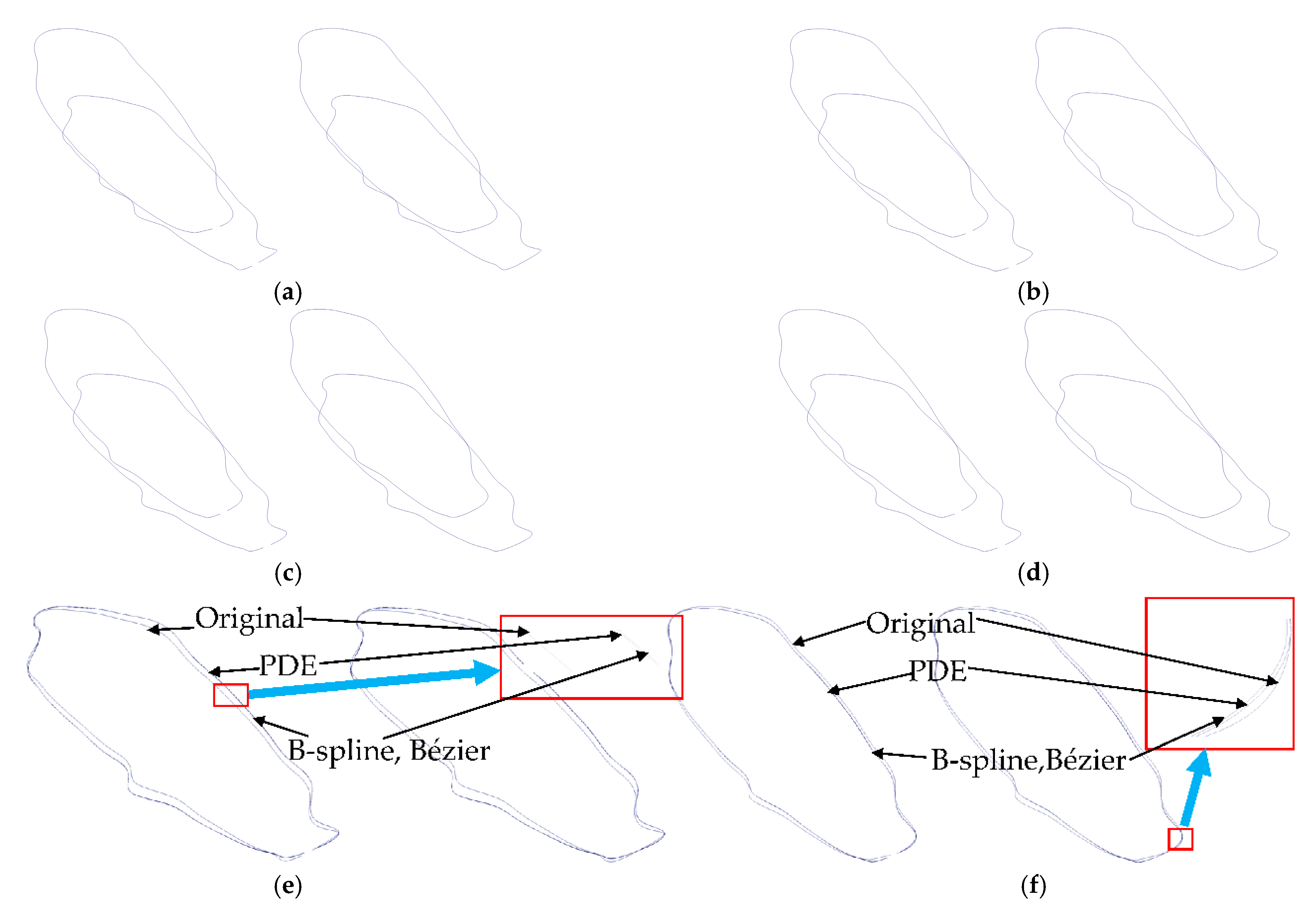
5.1. Comparison with Bézier and B-Spline Static Representations

In this section, we compare our proposed dynamic reconstruction method with Bézier and B-spline static reconstruction and give some examples to demonstrate the capacity of the proposed method in reconstructing complicated curves and its advantage in greatly reducing design variables through comparing the reconstructed curves with the original points used in the reconstruction. After that, we give two examples of reconstructing a 3D horse model and an armadillo model with the proposed method.

The proposed method is applicable to situations where the curves from two or more keyframes are used in Equation (5) to determine the eight unknown constants for dynamic curve reconstruction. In this paper, we consider the situation where only two curves, one from the first one and another from the second one of two keyframes, are used in Equation (5) to determine the eight unknown constants for dynamic curve reconstruction. For the comparison, two mathematical equations of Bézier curves defined in Equation (17) and two mathematical equations of B-spline curves defined in Equation (19) are used to reconstruct the same two curves.

The first example reconstructs a closed curve and its open version at the 20th frame and the 100th frame with our proposed dynamic reconstruction and Bézier and B-spline static reconstruction. Our proposed dynamic reconstruction method reconstructs the two curves: one at the 20th frame and the other at the 100th frame, with eight vector-valued design variables involved in one of the Equations from (5)–(8). In order to make the comparison fair, we use the same parametric values $u_n$ in our proposed dynamic reconstruction and Bézier and B-spline static reconstruction with four vector-valued design variables (coefficients), i.e., $k=3$ in Equations (17) and (19), leading to cubic Bézier and uniform cubic B-spline equations, to reconstruct each of the two curves. In total, eight design variables are involved in Bézier and B-spline static reconstruction. For the curve from the 20th keyframe, $t_j=t_0=0$ in Equation (5). For the 100th keyframe, $t_j=t_J=1$ in the same equation. Two Bézier equations defined in Equation (17) and two B-spline equations defined in Equation (19) are used to reconstruct the curve at the 20th frame and the curve at the 100th frame, respectively. The average and maximum errors between the points on the original curves and the corresponding points on the reconstructed curves are calculated with the following equations:

$$\begin{array}{c}{E}_{aj}=\frac{1}{N+1}{\displaystyle \sum _{n=0}^N}\frac{d_{jn}}{{\overline{d}}_{jn}}\\ E_{mj}=max\left\{\begin{array}{ccc}\frac{d_{j0}}{{\overline{d}}_{j0}}& \begin{array}{ccc}\frac{d_{j1}}{{\overline{d}}_{j1}}& \cdots & \frac{d_{jN}}{{\overline{d}}_{jN}}\end{array}& \frac{d_{jN}}{{\overline{d}}_{jN}}\end{array}\right\}\\ \left(j=0, 1\right)\end{array}$$

(23)

where

$$\begin{array}{c}{d}_{jn}=\sqrt{{\left[f_x\left(t_j, u_n\right)\right]}^2+{\left[f_y\left(t_j, u_n\right)\right]}^2+{\left[f_z\left(t_j, u_n\right)\right]}^2}\\ {\overline{d}}_{jn}=\sqrt{x_{j,n}{}^2+y_{j,n}{}^2+z_{j,n}{}^2}\\ \left(j=0, 1\right)\end{array}$$

(24)

and $f_x\left(t_j, u_n\right)$, $f_y\left(t_j, u_n\right)$, and $f_z\left(t_j, u_n\right)$ are determined by Equation (14) for our proposed dynamic reconstruction and the differences between the known $w_{j,n}$ and the corresponding ones obtained from Equation (17) for Bézier reconstruction and from Equation (19) for B-spline reconstruction.

The original and reconstructed curves are shown in Figure 3 where the curves shown on the left of (a), (b), (c), (d), (e), and (f) are open curves, the curves shown on the right of (a), (b), (c), (d), (e), and (f) are closed curves, and “PDE” stands for our proposed dynamic reconstruction method. In the figure, (a) shows the original curves at the 20th frame and 100th frame, (b) is the reconstructed curves with our proposed dynamic reconstruction method, (c) gives the reconstructed curves with Bézier static reconstruction, (d) shows the reconstructed curves with B-spline static reconstruction, (e) depicts the original curves and reconstructed ones at the 20th frame with our proposed dynamic reconstruction method and Bézier and B-spline static reconstruction, and (f) indicates the original curves and reconstructed ones at the 100th frame with our proposed dynamic reconstruction method and Bézier and B-spline static reconstruction. The original curves depicted in Figure 3a have complicated shapes. In spite of this, Figure 3e,f show the reconstructed curves with our proposed method approximate the original ones well. Figure 3e,f also show the reconstructed curves with our proposed method look the same as those reconstructed with Bézier and B-spline methods. In some local regions, they are slightly closer to the original curves than those reconstructed with B-spline and Bézier methods. Our proposed reconstruction method only involves eight vector-valued unknown constants, which are 5.7% of the design variables of the original curves. It indicates that the proposed method has a strong ability in reconstructing complicated open and closed curves with few design variables.

Table 2. Design variables, errors ($\times {10}^{-3}$), and computational time (CPU) for reconstruction shown in Figure 3.

		PM	PBB	${\mathit{E}}_{\mathit{A}1}$	${\mathit{E}}_{\mathit{A}2}$	${\mathit{E}}_{\mathit{A}12}$	${\mathit{E}}_{\mathit{m}1}$	${\mathit{E}}_{\mathit{m}2}$	${\mathit{E}}_{\mathit{m}12}$	CPU (ms)
PDE	OC	140	8	4.641821	3.811424	4.226623	71.60692	7.954821	71.60692	5.7532
B-spline	OC	140	8	4.631861	3.813969	4.222915	79.84222	7.796782	79.84222	3.3210
Bézier	OC	140	8	4.631861	3.813969	4.222915	79.84222	7.796782	79.84222	2.8257
PDE	CC	142	8	4.624602	3.810121	4.217362	71.00726	7.620819	71.00726	5.8322
B-spline	CC	142	8	4.615302	3.811597	4.213450	71.01385	7.470214	71.01385	3.5928
Bézier	CC	142	8	4.615302	3.811597	4.213450	71.01385	7.470214	71.01385	2.9644

gives a comparison of the number of design variables and average and maximum errors among the original curves and the reconstructed curves with our proposed dynamic reconstruction and Bézier and B-spline static reconstruction. The table also compares the computational time (CPU) used in reconstructing the curves. In the table, OC and CC indicate open curves and closed curves, respectively. PM is the total number of points on the two curves obtained from the 20th and 100th keyframes. PBB is the total number of vector-valued coefficients involved in Equation (5) and the total number of vector-valued coefficients used to reconstruct the two curves at the 20th and 100th frames with Equations (17) and (19). $E_{A1}$ and $E_{m1}$ are the average error and maximum error between the original and reconstructed curves at the 20th keyframe, $E_{A2}$ and $E_{m2}$ are the average error and maximum error between the original and reconstructed curves at the 100th keyframe, $E_{A12}$ is the average value of the average errors at the 20th and 100th keyframes, $E_{m12}$ is the bigger one of the maximum errors at the 20th and 100th keyframes, and all the errors in the table are multiplied by ${10}^{-3}$. The average errors $E_{A1}$ and $E_{A2}$ and maximum errors $E_{m1}$ and $E_{m2}$ are determined by the first one and second one of Equation (23), respectively.

The data shown in Table 2 indicate that both average errors and maximum errors from our proposed dynamic reconstruction method are small and almost same as those from Bézier and B-spline static reconstruction except for the maximum error for the open curve. The results from Bézier and B-spline static reconstruction are exactly the same. For the open curve, the maximum error from our proposed method is 71.60692, which is smaller than the maximum error from Bézier and B-spline static reconstruction at 79.84222. The computational time of our proposed dynamic reconstruction method is approximately two times that of Bézier static reconstruction and from 1.6–1.7 times that of B-spline static reconstruction.

The curve at the 20th frame and the corresponding curve at the 100th frame used in the above reconstruction are far away. In spite of this, our proposed dynamic reconstruction method still gives good reconstruction accuracy. When the two frames are closer, the errors can be significantly reduced. Here, we use two adjacent frames shown in Figure 4 to demonstrate this. The two adjacent frames used in this example are the 37th and 38th. The obtained results are given in Figure 4, which are organised in the same way as Figure 3. Figure 4e,f also clearly show that the reconstructed curves from our proposed dynamic reconstruction and Bézier and B-spline static reconstruction are very close to the original curves.

The average and maximum errors caused by our proposed dynamic reconstruction and Bézier and B-spline static reconstruction are given in

Table 3. Design variables, errors ($\times {10}^{-4}$), and computational time (CPU) for reconstruction shown in Figure 4.

		PM	PBB	${\mathit{E}}_{\mathit{A}1}$	${\mathit{E}}_{\mathit{A}2}$	${\mathit{E}}_{\mathit{A}12}$	${\mathit{E}}_{\mathit{m}1}$	${\mathit{E}}_{\mathit{m}2}$	${\mathit{E}}_{\mathit{m}12}$	CPU (ms)
PDE	OC	132	8	2.638812	3.142145	2.890479	8.422275	19.07610	19.07610	5.4184
B-spline	OC	132	8	2.172167	2.181193	2.176680	80.48240	80.82564	80.48240	3.0592
Bézier	OC	132	8	2.172167	2.181193	2.176680	80.48240	8.082564	80.48240	2.6934
PDE	CC	134	8	2.632932	3.169087	2.901010	8.077028	18.39898	18.39898	5.4873
B-spline	CC	134	8	2.186633	2.195735	2.191184	80.73569	81.08065	81.08065	3.1072
Bézier	CC	134	8	2.186633	2.195735	2.191184	80.73569	81.08065	81.08065	2.8346

. In the table, all the errors are multiplied by ${10}^{-4}$. The average errors caused by our proposed dynamic reconstruction are very small and slightly larger than those caused by Bézier and B-spline static reconstruction. The maximum errors of our proposed dynamic reconstruction are much smaller than those of Bézier and B-spline static reconstruction, i.e., 8.077028$~$8.422275 against 80.48240$~$80.73569 and 18.39898$~$19.07610 against 80.82564$~$81.08065. Once again, the computational time of our proposed method is higher than Bézier and B-spline static reconstruction, i.e., 1.9–2.01 times that of Bézier static reconstruction and 1.77–1.94 times that of B-spline static reconstruction.

The above discussions indicate that the errors caused by our proposed dynamic reconstruction method are almost as small as those caused by Bézier and B-spline static reconstruction. Bézier and B-spline static reconstruction do not involve the time variable in the reconstruction functions and are not applicable to dynamic and time-dependent reconstruction. In contrast, our proposed method can effectively tackle this problem.

Finally, we give two examples of reconstructing dynamic 3D models with our proposed dynamic reconstruction and B-spline static reconstruction. Except that Bézier static reconstruction is slightly faster than B-spline static reconstruction, Bézier static reconstruction gives the exactly results as B-spline static reconstruction. Due to this reason, Bézier static reconstruction will not be considered in the following examples.

The first example is to reconstruct deformed shapes of a horse model at different keyframes obtained from the simulations of position-based dynamics. To this aim, the curves to be reconstructed are first extracted from undeformed polygon models. As shown in Figure 5, the curves to be reconstructed shown in (b) are extracted from the undeformed polygon horse model in (a). The original horse model has 15,389 vertices and 30,710 faces. Since each vertex has three components x, y, and z, the original horse model has 46,167 design variables in total. To represent the horse model, 593 curves have been extracted, and 4744 vector-value coefficients involved in Equation (5) are used to define the 593 curves at two different keyframes. Since each vector-valued coefficient has three components x, y, and z, the proposed method uses, in total, 14,232 unknown constants (design variables) to reconstruct the horse model at two different keyframes. Although the 593 curves are manually extracted, and the number of points on each of the extracted curves has not been optimised to reduce the number of the extracted curves and accordingly decrease the number of the unknown constants, the extracted curves still reduce more than two-thirds of the design variables of the polygon horse model.

Figure 6 shows the original deformed models and the reconstructed ones with our proposed method and B-spline method. In the figure, the “PDE model” is obtained from our proposed dynamic reconstruction, the “B-spline model” is obtained with B-spline static reconstruction, the images in the first and fourth rows are the original deformed models obtained with PBD simulations, while those in the second and fifth rows are reconstructed by our proposed dynamic reconstruction and the ones in the third row and sixth row are reconstructed with B-spline static reconstruction. Comparing the original models in the first and fourth rows to the reconstructed models with our proposed dynamic reconstruction in the second and fifth rows and B-spline static reconstruction in the third and sixth rows, we could not find any visible differences. We have also calculated the average and maximum errors between the reconstructed models obtained with the two methods and the original deformed models. The average error and maximum error of using our proposed method to reconstruct the first and tenth frames are $6.1746\times {10}^{-4}$ and $4.672209\times {10}^{-2}$, and the average error and maximum error of using B-spline method to reconstruct these two frames are $5.321225\times {10}^{-4}$ and $5.191078\times {10}^{-2}$. These data also indicate that our proposed method and B-spline have almost same reconstruction accuracy. The average errors from our proposed method and B-spline method are small as they are three to four orders of magnitude lower than the differences between the maximum and minimum x, y, and z coordinates. It indicates that the proposed method has good reconstruction accuracy.

We have calculated the CPU time of using PBD to obtain the deformed shapes at 100 keyframes. In total, 6420 milliseconds were required in the PBD simulation. In contrast, our proposed method takes 1827 milliseconds to reconstruct the deformed shapes at two keyframes and generate 98 new deformed shapes between the two keyframes by setting the time variable $t$ in Equation (5) to 98 different values. Clearly, using our proposed dynamic reconstruction to replace PBD simulations at some keyframes can reduce the time of PBD simulations.

The second example is to reconstruct deformed shapes of an armadillo polygon model at different keyframes obtained from the simulations of position-based dynamics. The original armadillo model has 5182 vertices and 5180 faces, leading to 5182 vector-valued design variables. In total, 196 curves were extracted to represent the armadillo model, and 1568 vector-value coefficients involved in Equation (5) are used to define the 196 curves at two different keyframes. Once again, our proposed method reduces the vector-valued design variables of the armadillo polygon model by more than two-thirds.

Figure 7 shows the original deformed shapes of the armadillo polygon model and the reconstructed ones with our proposed method and B-spline method. Comparing the original deformed shapes and those reconstructed with our method and B-spline method, we could not find any visible differences. This example also indicates that our proposed method has good reconstruction accuracy.

5.2. Limitations of This Work

There are some limitations to the method proposed in this paper. Here, we identify these limitations. In the following section, we discuss how to tackle these limitations.

The first limitation is that the extracted curves are not optimal. In this paper, the curves used to represent the horse model were manually extracted without any optimization. This has two problems. The first one is that some curves may have too few vertices, and others may have too many vertices. Too few vertices cannot maximize the potential of the proposed approach in reducing design variables. Too many vertices may lead to large errors. The second one is that manually extracted curves are not proper in demonstrating the advantage of the proposed approach in reducing design variables since it cannot automatically increase or decrease the number of points on a curve according to a given reconstruction error.

The second limitation is that the number and position of the keyframes have not been optimized. In this paper, only the models from two keyframes are reconstructed. How many keyframes and which keyframes are optimal for reconstruction have not been investigated.

The third limitation is that reconstructing dynamic 3D models subjected to a given error threshold has not been examined. As it can be observed from Figure 3 and Figure 4 and the data in Table 2 and Table 3, there are some reconstruction errors, which may not meet the requirements of some applications where high accuracy is essential.

6. Conclusions and Future Work

In this paper, we have developed a new method to reconstruct dynamic 3D models obtained from position-based dynamics simulation. We have integrated the governing equation describing the bending deformations of elastic beams and Newton’s second law describing object motion to develop the mathematical model for the reconstruction of dynamic 3D models, used the separation of variables to obtain the closed-form solution of the mathematical model, and applied the obtained closed-form solution to generate reconstructed 3D models at different frames. We have also compared the reconstructed curves to the original polygon vertices and those reconstructed with Bézier and B-spline static reconstruction, and the reconstructed models with our method and B-spline method to the original deformed models at different keyframes. These comparisons demonstrate that the proposed method has good reconstruction accuracy and a small data size.

The work presented in this paper only used the closed-form solution of the proposed mathematical model to reconstruct deformed models at different keyframes obtained from the simulation of position-based dynamics. However, the proposed method can also be used to create new deformed models at new frames by setting the time variable $t$ to different values between $0\le t\le 1$, which have not been generated with position-based dynamics. With such applications, many keyframes simulated with position-based dynamics can be replaced with the dynamic ODE-based simulation to reduce the computational time spent on the simulation with position-based dynamics. We will investigate this in our following work.

Secondly, we will investigate an automatic and optimal curve extraction method. With this method, a curve reconstruction maximum error $E_{max}$ is first specified. Subjected to the limitation of $E_{max}$, the vertices for one curve are automatically identified, and the reconstruction error $E_{rec}$ is calculated and compared with $E_{max}$. If $E_{rec}$ is less than $E_{max}$, more vertices are added to the curve. If $E_{rec}$ is larger than $E_{max}$, some vertices on the curve are removed. The process is repeated until $E_{rec}$ is not larger than $E_{max}$.

Thirdly, we will develop an optimization method to obtain the optimal number of keyframes used in the reconstruction and decide which keyframes should be selected for reconstruction. In doing so, PDE-based dynamic deformations are combined with the simulation of position-based dynamics to reduce the keyframes for reconstruction and raise the computational efficiency of position-based dynamics while keeping the same simulation accuracy.

Fourthly, we will propose two approaches to tackle the problem of reconstructing dynamic 3D models subjected to a given error threshold. One approach is to divide one curve into two or more curves to reduce reconstruction errors until a given error threshold is reached, and the other approach is to add more terms to Equations (5)–(8) through changing $m_{w0}$, $D_{w0}$, and $D_{w1}$ into $m_{wk}$, $D_{wk}$, and $D_{wk}$ ($k=1, 2, 3,\dots$) to satisfy the requirement of a given error threshold.

References

1. Magnenat-Thalmann, N.; Laperrire, R.; Thalmann, D. Joint-dependent local deformations for hand animation and object grasping. In Proceedings of Graphics Interface ’88; Canadian Information Processing Society: Mississauga, ON, Canada, 1988. [Google Scholar]
2. Kavan, L.; Collins, S.; Žára, J.; O’Sullivan, C. Geometric skinning with approximate dual quaternion blending. ACM Trans. Graph. 2008, 27, 1–23. [Google Scholar] [CrossRef]
3. Mancewicz, J.; Derksen, M.L.; Rijpkema, H.; Wilson, C.A. Delta Mush: Smoothing deformations while preserving detail. In Proceedings of the Fourth Symposium on Digital Production; Association for Computing Machinery: New York, NY, USA, 2014; pp. 7–11. [Google Scholar]
4. Le, B.H.; Lewis, J.P. Direct Delta Mush Skinning and Variants. ACM Trans. Graph. 2019, 38, 113. [Google Scholar] [CrossRef]
5. Le, B.H.; Villeneuve, K.; Gonzalez-Ochoa, C. Direct delta mush skinning compression with continuous examples. ACM Trans. Graph. 2021, 40, 72. [Google Scholar] [CrossRef]
6. Lewis, J.P.; Cordner, M.; Fong, N. Pose space deformation: A unified approach to shape interpolation and skeleton-driven deformation. In Proceedings of the 27th Annual Conference on Computer Graphics and Interactive Techniques; ACM Press/Addison-Wesley Publishing Co.: New York, NY, USA, 2000; pp. 165–172. [Google Scholar]
7. Mohr, A.; Gleicher, M. Building efficient, accurate character skins from examples. ACM Trans. Graph. 2003, 22, 562–568. [Google Scholar] [CrossRef]
8. Le, B.H.; Deng, Z. Smooth skinning decomposition with rigid bones. ACM Trans. Graph. 2012, 31, 199. [Google Scholar] [CrossRef]
9. Bailey, S.W.; Otte, D.; Dilorenzo, P.; O’Brien, J.F. Fast and deep deformation approximations. ACM Trans. Graph. 2018, 37, 119. [Google Scholar] [CrossRef]
10. Xu, Z.; Zhou, Y.; Kalogerakis, E.; Landreth, C.; Singh, K. RigNet: Neural rigging for articulated characters. ACM Trans. Graph. 2020, 39, 58. [Google Scholar] [CrossRef]
11. Nealen, A.; Müller, M.; Keiser, R.; Boxerman, E.; Carlson, M. Physically based deformable models in computer graphics. Comput. Graph. Forum 2006, 25, 809–836. [Google Scholar] [CrossRef]
12. Waters, K. A muscle model for animation three-dimensional facial expression. ACM SIGGRAPH Comput. Graph. 1987, 21, 17–24. [Google Scholar] [CrossRef]
13. Terzopoulos, D.; Platt, J.; Barr, A.; Fleischer, K. Elastically deformable models. In Proceedings of the 14th Annual Conference on Computer Graphics and Interactive Techniques; Association for Computing Machinery: New York, NY, USA, 1987; pp. 205–214. [Google Scholar]
14. Eymard, R.; Gallouët, T.; Herbin, R. Finite volume methods. In Handbook of Numerical Analysis; Elsevier: Amsterdam, The Netherlands, 2000; Volume 7, pp. 713–1018. [Google Scholar]
15. Müller, M.; Heidelberger, B.; Hennix, M.; Ratcliff, J. Position based dynamics. J. Vis. Commun. Image Represent. 2007, 18, 109–118. [Google Scholar] [CrossRef] [Green Version]
16. Macklin, M.; Müller, M. Position based fluids. ACM Trans. Graph. 2013, 32, 1–2. [Google Scholar] [CrossRef]
17. Müller, M.; Dorsey, J.; McMillan, L.; Jagnow, R.; Cutler, B. Stable real-time deformations. In Proceedings of the 2002 ACM SIGGRAPH/Eurographics Symposium on Computer Animation, San Antonio, TX, USA, 21–22 July 2002; pp. 49–54. [Google Scholar]
18. Position Based Dynamics. Available online: https://github.com/InteractiveComputerGraphics/PositionBasedDynamics (accessed on 20 November 2021).
19. Li, J.; Yao, F.; Liu, Y.; Wu, Y. Reconstruction of Broken Blade Geometry Model Based on Reverse Engineering. In 2010 Third International Conference on Intelligent Networks and Intelligent Systems; IEEE Computer Society Press: Washington, DC, USA, 2010; pp. 680–682. [Google Scholar]
20. Prautzsch, H.; Wolfgang, B.; Marco, P. Bézier and B-spline Techniques; Springer: Berlin/Heidelberg, Germany, 2002; p. 6. [Google Scholar]
21. Patrikalakis, N.M.; Maekawa, T. Shape Interrogation for Computer Aided Design and Manufacturing; Springer: Berlin/Heidelberg, Germany, 2002; p. 15. [Google Scholar]
22. Hoschek, J.; Lasser, D. Fundamentals of Computer Aided Geometric Design; AK Peters Ltd.: Natick, MA, USA, 1993. [Google Scholar]
23. Gálvez, A.; Iglesias, A. Particle swarm optimisation for non-uniform rational B-spline surface reconstruction from clouds of 3D data points. Inf. Sci. 2012, 192, 174–192. [Google Scholar] [CrossRef]
24. You, L.H.; Yang, X.S.; Pachulski, M.; Zhang, J.J. Boundary constrained swept surfaces for modelling and animation. Comput. Graph. Forum 2007, 26, 313–322. [Google Scholar] [CrossRef]
25. You, L.H.; Ugail, H.; Tang, B.P.; Jin, X.; You, X.Y.; Zhang, J.J. Blending using ODE swept surfaces with shape control and C1 continuity. Vis. Comput. 2014, 30, 625–636. [Google Scholar] [CrossRef] [Green Version]
26. Chaudhry, E.; You, L.H.; Jin, X.; Yang, X.S.; Zhang, J.J. Shape modeling for animated characters using ordinary differential equations. Comput. Graph. 2013, 37, 638–644. [Google Scholar] [CrossRef]
27. Bloor, M.I.; Wilson, M.J. Using partial differential equations to generate free-form surfaces. Comput. Aided Des. 1990, 22, 202–212. [Google Scholar] [CrossRef]
28. Ugail, H.; Bloor, M.I.G.; Wilson, M.J. Techniques for interactive design using the PDE method. ACM Trans. Graph. 1999, 18, 195–212. [Google Scholar] [CrossRef]
29. Ugail, H.; Kirmani, S. Method of surface reconstruction using partial differential equations. In Proceedings of the 10th WSEAS International Conference on Computers, Athens, Greece, 13–15 July 2006; pp. 51–56. [Google Scholar]
30. Bian, S.H.; Deng, Z.; Chaudhry, E.; You, L.H.; Yang, X.S.; Guo, L.; Ugail, H.; Jin, X.; Xiao, Z.D.; Zhang, J.J. Efficient and realistic character animation through analytical physics-based skin deformation. Graph. Models 2019, 104, 201035. [Google Scholar] [CrossRef]
31. Wang, S.B.; Xiang, N.; Xia, Y.; You, L.H.; Zhang, J.J. Real-time surface manipulation with C1 continuity through simple and efficient physics-based deformations. Vis. Comput. 2021, 37, 2741–2753. [Google Scholar] [CrossRef]
32. Yun, S.; Sourin, A.; Castro, G.G.; Ugail, H. A PDE method for patchwise approximation of large polygon meshes. Vis. Comput. 2010, 26, 975–984. [Google Scholar]
33. Bender, J.; Müller, M.; Macklin, M. A survey on position based dynamics. In Proceedings of the European Association for Computer Graphics: Tutorials, Lyon, France, 24–28 April 2017; pp. 1–31. [Google Scholar]
34. Müller, M.; Keiser, R.; Nealen, A.; Pauly, M.; Gross, M.; Alexa, M. Point based animation of elastic, plastic and melting objects. In Proceedings of the 2004 ACM SIGGRAPH/Eurographics Symposium on Computer Animation, Grenoble, France, 27–29 August 2004; pp. 141–151. [Google Scholar]
35. Bender, J.; Koschier, D.; Charrier, P.; Weber, D. Position-based simulation of continuous materials. Comput. Graph. 2014, 44, 1–10. [Google Scholar] [CrossRef]
36. Macklin, M.; Müller, M.; Chentanez, N. XPBD: Position-based simulation of compliant constrained dynamics. In Proceedings of the 9th International Conference on Motion in Games, Burlingame, CA, USA, 10–12 October 2016; pp. 49–54. [Google Scholar]
37. Hong, M.; Jung, S.; Choi, M.H.; Welch, S.W. Fast volume preservation for a mass-spring system. IEEE Comput. Graph. Appl. 2006, 26, 83–91. [Google Scholar] [CrossRef]
38. Irving, G.; Schroeder, C.; Fedkiw, R. Volume conserving finite element simulations of deformable models. ACM Trans. Graph. 2007, 26, 13-es. [Google Scholar] [CrossRef]
39. Kakadiaris, I.A. Physics-Based Modeling, Analysis and Animation; Technical Reports No. MS-CIS-93-45; University of Pennsylvania: Philadelphia, PA, USA, 1993. [Google Scholar]
40. Kadleček, P.; Ichim, A.-E.; Liu, T.; Křivánek, J.; Kavan, L. Reconstructing personalised anatomical models for physics-based body animation. ACM Trans. Graph. 2016, 35, 213. [Google Scholar] [CrossRef] [Green Version]
41. Bender, J.; Müller, M.; Macklin, M. Position-based simulation methods in computer graphics. In Proceedings of the 36th Annual Conference of the European Association for Computer Graphics, Eurographics 2015—Tutorials, Zurich, Switzerland, 4–8 May 2015. [Google Scholar]
42. Barrielle, V.; Stoiber, N.; Cagniart, C. BlendForces: A dynamic framework for facial animation. Comput. Graph. Forum 2016, 35, 341–352. [Google Scholar] [CrossRef]
43. Barrielle, V.; Stoiber, N. Realtime performance-driven physical simulation for facial animation. Comput. Graph. Forum 2019, 38, 151–166. [Google Scholar] [CrossRef] [Green Version]
44. Xu, L.; Lu, Y.; Liu, Q. Integrating viscoelastic mass spring dampers into position-based dynamics to simulate soft tissue deformation in real time. R. Soc. Open Sci. 2018, 5, 1–16. [Google Scholar] [CrossRef] [Green Version]
45. Kozlov, Y.; Bradley, D.; Bächer, M.; Thomaszewski, B.; Beeler, T.; Gross, M. Enriching facial blendshape rigs with physical simulation. Comput. Graph. Forum 2017, 36, 75–84. [Google Scholar] [CrossRef]
46. Guo, J.; Li, J.; Narain, R.; Park, H.S. Inverse simulation: Reconstructing Dynamic Geometry of Clothed Humans via Optimal Control. In Proceedings of the 2021 IEEE/CVF Conference on Computer Vision and Pattern Recognition (CVPR), Nashville, TN, USA, 20–25 June 2021; pp. 14693–14702. [Google Scholar]
47. Gladilin, E.; Zachow, S.; Deuflhard, P.; Hege, H.-C. Anatomy- and physics-based facial animation for craniofacial surgery simulations. Med. Biol. Eng. Comput. 2004, 42, 167–170. [Google Scholar] [CrossRef]
48. Bauchau, O.A.; Craig, J.I. Euler-Bernoulli beam theory. In Structural Analysis; Springer: Dordrecht, The Netherlands, 2009; pp. 173–221. [Google Scholar]
49. Polyanin, A.D.; Zhurov, A.I. Separation of Variables and Exact Solutions to Non-Linear PDEs; CRC Press; Taylor & Francis Group, LLC: Boca Raton, FL, USA, 2022; pp. 1–2. [Google Scholar]
50. Abdel-Aziz, H.S.; Zanaty, E.A.; Ali, H.A.; Saad, M.K. Generating Bézier curves for medical image reconstruction. Results Phys. 2021, 23, 103996. [Google Scholar] [CrossRef]
51. Ravari, A.N.; Taghirad, H.D. Reconstruction of B-spline curves and surfaces by adaptive group testing. Comput. Aided Des. 2016, 74, 32–44. [Google Scholar] [CrossRef]
Figure 1. Dog model with different vertices and faces. (a) 502 vertices and 1000 faces, (b) 2002 vertices and 4000 faces, (c) 10,002 vertices and 20,000 faces, (d) 49,714 vertices and 99,424 faces.
Mathematics 10 00821 g001
Figure 2. PBD deformation results of our horse model. From the first to the last pose, they are frame 1, 20, 30, 40, 50, 60, 70, 80, 90, 100. The simulation results demonstrate that PBD has a high-quality visual deformation performance.
Mathematics 10 00821 g002
Figure 3. Original and reconstructed curves with 71 points at 20th and 100th frames. (a) Original curves at 20th, 100th frames. (b) PDE reconstructed curves at 20th, 100th frames. (c) B-spline reconstructed curves at 20th, 100th frames. (d) Bézier reconstructed curves at 20th, 100th frames. (e) Original, PDE, B-spline, and Bézier curves at 20th frame. (f) Original, PDE, B-spline, and Bézier curves at 100th frame.
Mathematics 10 00821 g003
Figure 4. Original and reconstructed curves with 67 points at 37th and 38th frames. (a) Original curves at 37th, 38th frames. (b) PDE reconstructed curves at 37th, 38th frames. (c) B-spline reconstructed curves at 37th, 38th frames. (d) Bézier reconstructed curves at 37th, 38th frames. (e) Original, PDE, B-Spline, and Bézier curves at 37th frame. (f) Original, PDE, B-Spline, and Bézier curves at 38th frame.
Mathematics 10 00821 g004
Figure 5. Undeformed horse model and extracted curves. (a) Polygon horse model, (b) extracted curves.
Mathematics 10 00821 g005
Figure 6. Original deformed shapes and reconstructed shapes of a horse model at keyframes 1, 20, 30, 40, 50, 60, 70, 80, 90, and 100.
Mathematics 10 00821 g006
Figure 7. Original deformed shapes and reconstructed shapes of an armadillo model at keyframes 1, 20, 30, 40, 50, 60, 70, 80, 90, and 100.
Mathematics 10 00821 g007