Abstract
The present work investigates the influence of triple diffusion on Carreau nanoliquid in peristaltic flow through an asymmetric channel. By using appropriate non-dimensional parameters, governing equations are transformed to conventional non-linear partial differential equations. The Ms-DTM is used to find solutions to developing equations. Because of the buoyancy force that prevails inside the boundary layer, velocity is impacted by the buoyancy ratio. The current investigation found that as the varied values of the modified Dufour parameter were increased, the temperature profile increased. The thermal conductivity increases as thermal diffusivity increases. It has also been discovered that the existence of triple-diffusing components with low diffusivity might alter the type of convection in the system. Graphs depict the influence of several parameters on velocity, salt1 and salt2 concentrations, solute concentration, and temperature.
MSC:
76XX; 76AXX; 76DXX; 76RXX; 76VXX; 35S16
1. Introduction
Natural convection with multi-diffusive features has several practical applications. The triple diffusion motion may be found in many scientific and technical fields, including astrophysics, nuclear waste disposal, geology, chemical engineering, and the study of deoxyribonucleic acid (DNA). Ghalambaz et al. [1] analyzed triple diffusion in a porous cavity that is a mixing process, in which three stratifying factors with different diffusivities, such as heat and salt concentration, control the density. When the thermal expansion coefficient and element concentration in the mixture alter sufficiently, the buoyancy force induced by mass transfer can have a major influence on transport circulation and component distribution in the cavity. The number of buoyancy forces increases as the number of components increases, and the mixture’s behavior becomes more complicated. Furthermore, Archana et al. [2] investigated the impact of buoyancy force and nonlinear thermal radiation on triple diffusion flow down a horizontal plate using the Casson nanofluid model. Khan et al. [3,4] investigated the effect of triple diffusion in porous media. Umavathi et al. [5] expanded the study by investigating the convective flow of triple diffusion under robin boundary conditions in a vertical flat plate. Nawaz et al. [6] numerically investigated the nanoparticle’s twofold diffusion and the influence of thermal diffusion.
Latham [7] described peristalsis in 1966. The Greek term for “peristalsis” is peristaltikos, which means “clasping and compression”. The mechanism of peristalsis occurs in the intestines and ureters, and the motion of blood in small vessels like capillaries, venules, and arterioles. In the nuclear industry, a toxic liquid can be pumped peristaltically to avoid pollution of the environment. Differential equations are increasingly being employed in physical sciences like liquid transport, microelements, radiation analysis, heat convection and conduction, and dynamics. Partial differential equations aid in the mathematical formulation of engineering and physical problems. Further, Shapiro et al. [8] analyzed peristaltic motion with low Reynolds number and long wavelengths. Jaffrin et al. [9] expanded peristaltic transport. Vajravelu et al. [10] demonstrated the peristaltic flow of the Carreau model under the influence of multislip parameters. Reddy et al. [11] demonstrated the peristaltic motion of a Carreau liquid under the influence of porous material and an induced magnetic field. Nadeem et al. [12] demonstrated the peristaltic pumping of Carreau liquid. Hayat et al. [13] analyzed the influence of induced magnetic field on Carreau liquid in peristaltic pumping.
In 1995, Choi [14] of Argonne National Laboratory coined the term “nanofluid” after discovering nanoliquids. Nanoparticles have applications in a wide range of sectors, such as industry, biology, chemistry, and photochemistry. The present advancement of nanofluids has received a lot of interest because of its applications. Furthermore, Asha et al. [15] analyzed the impact of joule heating in the mechanism of peristalsis of Carreau nanoliquid in an inclined asymmetric channel. Eldabe et al. [16] explained the mechanism of peristalsis of Carreau nanoliquid under the impact of mass and heat transfer. Machireddy et al. [17] demonstrated MHD Carreau liquid with the impact of cross-diffusion and heat and mass transfer. Akram et al. [18] studied the influence of inclined magnetic field and nanofluid on peristaltic motion of carreau fluid model.
In recent years, there has been a surge of attentiveness in developing and applying analytical and numerical approaches. Such strategies can aid in overcoming the complexity and non-linearity seen in non-Newtonian liquids. Mechanisms of peristalsis with non-Newtonian liquids necessitate substantially non-linear partial differential equations. It is hard to find precise answers to such challenges. In this research, we employed a semi-analytical technique known as the differential transform method (DTM). In 1986, Zhou was the first to introduce DTM [19]. The multi-step differential transformation approach (Ms-DTM) is a dependable semi-analytical method that is an excellent enhancement over the traditional DTM. Furthermore, Odibat et al. [20] demonstrated the multi-step differential transform method and its appliances to chaotic or non-chaotic systems. Hasona et al. [21] studied the influence of Joule heating on Jeffery liquid in the mechanism of peristalsis using Ms-DTM. Hasona et al. [22] analyzed Williamson nanoliquids in an asymmetric channel using Ms-DTM. Hasona et al. [23] studied the combined impact of temperature-dependent viscosity and MHD on peristaltic pumping of Jeffrey nanoliquid. Tripathi et al. [24] described DTM in peristaltic viscoelastic bioliquid motion in an asymmetric porous channel. Hatami et al. [25] analyzed third-grade non-Newtonian blood transport in arteries using Ms-DTM. Beg et al. [26] investigated multi-step DTM in the mechanism of magneto-peristaltic motion of a conducting Williamson viscoelastic liquid.
This study aims to provide different predictions about the effect of natural convection with triple-diffusive features on the mechanism of peristalsis of Carreau nanoliquid through an asymmetric channel. Because of the buoyancy force that prevails inside the boundary layer, velocity is impacted by the buoyancy ratio. The current investigation found that as the varied values of the modified Dufour parameter were increased, the temperature profile increased. The thermal conductivity increases as thermal diffusivity increases. It has also been discovered that the existence of triple-diffusing components with low diffusivity might alter the type of convection in the system. Ms-DTM is used to find solutions, and graphs depict the influence of several parameters on velocity, salt1 and salt2 concentrations, and temperature.
2. Mathematical Analysis
As illustrated in Figure 1, Carreau nanoliquid peristaltic movements propagate in a two-dimensional asymmetric channel with a sinusoidal wave near the flexible and non-conducting walls. Now, () are taken as Cartesian coordinate systems. The mathematical model of the channel surface of the wall is [20].
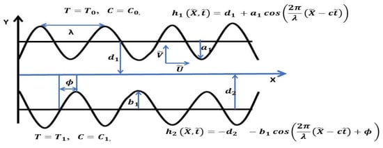
Figure 1.
Physical configuration.
Here, and denote waves amplitudes, denote channel widths, denotes the length of the wave, denotes the propagation of velocity, represents time, represents the direction of wave propagation, and represents phase difference, which varies in the range . A symmetric channel with waves out of the phase is given, and the waves that are in phase are given as .
Here, and satisfy the following condition:
Let be the velocity field defined as follows:
Here, and are components of velocity, respectively.
The constitutive equations [13] of Carreau liquid are given as follows:
stands for infinite shear rate viscosity, for zero shear rate viscosity, and for the time constant; n represents power-law index with no dimension; and is given as follows:
where is the strain tensor of the second invariant. Note that the power-law index characterizes the fluid behavior, and fluid is characterized as shear thinning for , shear thickening for , and Newtonian fluid for and/or . For large values of , the power-law model can be obtained.
Carreau liquid’s governing equations [2,18] are given below.
The wave frame and the laboratory frame have a relationship that is defined by the following:
In a wave frame, represents velocity components, and denotes coordinates.
Introducing, non-dimensional quantities as following:
where θ, Ω1, Ω2, and Ω are the dimensionless temperature, solutal concentration 1, solutal concentration 2, and solutal concentration, respectively.
Using the non-dimensional variables mentioned above, the basic Equations (6)–(10) were reduced to
Removing pressure from Equations (19) and (20) provides
where represents a parameter of Brownian motion, represents a parameter of thermophoresis, represents thermal Grashof number, represents solutal Grashof number, and represent the buoyancy ratios of concentration 1 and concentration 2, and and indicate the modified Dufour parameters of concentration 1 and concentration 2. and represent the Dufour solutal Lewis numbers of concentration 1 and concentration 2.
The boundary constraints with no dimension in the problem’s wave frame are given as follows:
where and satisfy the condition
In the wave frame, the average flux with no dimension is given as
In the wave frame, the mean time is given by .
Using the boundary conditions (26), Equations (19)–(25) are solved by using Ms-DTM with symbolic Mathematica tools.
2.1. Multi-Step Differential Transformation Method
Take domain T, in which is an analytical function, and any point can be represented in T. A power series is then used to express the function, with the center at . The function can be transformed into a differential transformation as given below.
Here, and are the original function and transformed function, respectively. The conversion of the inverse is written as
The Equations (28) and (29) give
A finite series gives the function and Equation (28) presented below.
Here, is ignored because it is too small. The value of m depends on the convergence of the series coefficients.
The value of m is considered up to m = 15 for finding the approximation solution. It was selected since beyond m = 15, there was no variation in the result.
2.2. Solution of the Problem by Ms-DTM
Here, we obtain the solution of Equations (19)–(25) with the appropriate boundary constraints (26) by using the Ms-DTM as follows:
where Ψ[k], Θ[k], Φ1 [k], Φ2 [k], and Φ[k] are the differential transformation functions of ψ(y), θ(y), Ω1(y), Ω2(y), and Ω(y), respectively, defined as follows:
The transformed forms of the boundary constraints are given as follows:
where , and unknown coefficients are to be found.
Putting Equation (42) into Equations (32)–(36), and further values of , , , , and , it is solved by recursive method. Hence, substituting all , , , , and into Equations (37)–(41), the obtained series solutions are as follows:
Differentiating Equation (42) partially for y, we get the velocity equation as follows:
Using boundary conditions of Equation (26), we can obtain the values of , and
Using boundary conditions of Equation (26), we can obtain the values of , and
A comparison between the solutions obtained by the Ms- DTM with exact solution is shown in Table 1.

Table 1.
Comparison of the solution obtained by Ms-DTM with the exact solution for .
3. Results and Discussion
The above description leads to a system of non-linear coupled partial differential equations. When solving explicitly, exact solutions are difficult to obtain. The problem at hand is approached semi-analytically by using Mathematica software’s Ms-DTM. The results obtained by Ms-DTM have been compared with the Exact solution. The results show that they matched nicely as can be seen from Table 1. In this paper, we discuss the influence of the Weisenberg number , the power-law index, Buoyancy ratio parameters and , modified Dufour parameters and , Dufour solutal Lewis numbers and , solutal Grashof number , Brinkman number , thermal Grashof number , parameter of thermophoresis , and parameter of Brownian motion on solutal concentration 1, solutal concentration 2, velocity, temperature, and solutal concentration profiles.
3.1. Velocity Distribution
The impact of , , , , , and on velocity profile are presented in Figure 2a–g. Figure 2a shows that velocity in peristaltic pumping decreases with an increase in . Physically, the Weissenberg number is the ratio of the relaxation time of the fluid and the specific process time. It grows with the thickness of fluid, and that is why the velocity of the fluid depreciates. Figure 2b explains the influence of the power-law index on the velocity profile, increasing the values and reducing the non-Newtonian behavior of the flow, and this leads to an enhancement of the momentum boundary layer. Figure 2c illustrates that the velocity in peristaltic pumping enhances with a rise in Brinkman number . In addition, Figure 2d shows that enhancing the thermal Grashof number decreases the velocity of the liquid. satisfies the proportionate influence of viscous hydrodynamic force and thermal buoyant force. In Figure 2e, an increase in the solutal Grashof number decreases the velocity distribution of the wall, as it influences the shrinkage of the thermal boundary layer. From Figure 2f,g, it can be observed that the velocity in peristaltic pumping rises with an increase in , due to the buoyancy force, which dominates within the boundary layer, as depends upon density, which decreases with increasing temperature. The buoyancy ratio is the ratio of fluid density contributions by the two solutes.
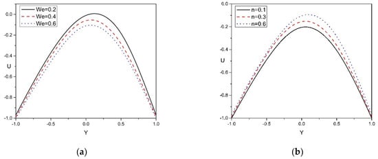
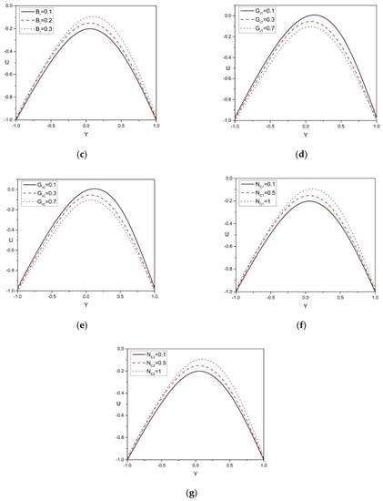
Figure 2.
(a–g): Velocity distribution versus Y for various physical parameters .
3.2. Temperature Distribution
Figure 3a–g are prepared to represent the temperature profile via , , , , , , and . Figure 3a–f demonstrates that the temperature distribution rises when there is a rise in , , , , and , respectively. Figure 3a demonstrates that the temperature distribution rises when there is a rise in because the arbitrary movement of the nanoparticle is increased as is increased, causing more heat in the liquid and thus enhancing the liquid’s temperature. From Figure 3b, it can be observed that the temperature distribution rises when there is a rise in . Furthermore, the presence of nanoparticles in the fluid is represented by these two parameters. Because these particles increase the fluid’s thermal conductivity, the temperature rises, and the thermal boundary layer thickens. From Figure 3c,d, it can be noticed that temperature distribution increases for the larger varying values of the modified Dufour parameters and . Thermal conductivity rises as thermal diffusivity rises, leading to an increase in molecular vibrations, and as a result, the temperature increases. From Figure 3e,f, it can be noticed that the temperature distribution increases for the larger varying values of Dufour solutal Lewis numbers and . Within the boundary layer, both the dimensionless temperature and Dofour solutal Lewis number are inversely proportional to the concentration difference at the wall. Therefore, the greater the Dofour solutal Lewis number, the larger will be the temperature distribution. Figure 3g represents the effect of the power-law index on the temperature distribution. The rise in the power-law index decreases the temperature distribution due to the reduced non-Newtonian behavior of the flow, and this leads to an enhancement of the momentum boundary layer.
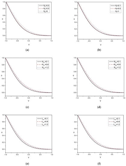
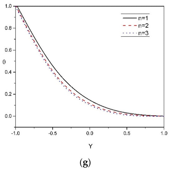
Figure 3.
(a–g): Temperature distribution versus Y for various physical parameters .
3.3. Concentration Distribution
Figure 4a–e shows that the solutal concentration profile 1 of the nanoparticle is influenced by , , , , and . Figure 4a,b shows that solutal concentration profile 1 in peristaltic motion increases by rising the values of and . Within the concentration boundary layer, both the solutal concentration 1 and Dofour solutal Lewis number are inversely proportional to the concentration difference at the wall. Therefore, the greater the Dofour solutal Lewis number, the larger will be solutal concentration 1. As a result of increased mass diffusivity, these parameters show a significant increase in solutal concentration profile 1 of the nanoparticle. Higher mass diffusivity indicates a higher possibility of molecular collision due to a large difference in solutal concentration. The difference in the solutal concentrations of molecules grows as the concentration gradient gets higher. Figure 4c shows that solutal concentration profile 1 in peristaltic motion increases by rising the values of . Figure 4d shows a substantial decrease in solutal concentration profile 1 of the nanoparticle by enhancing the Brownian motion parameter . Brownian motion is based on a random motion of liquid elements moving across a flow surface as nanoparticle movement is pushed from the hot region to the cold region, which results in a decrease in concentration distribution. Figure 4e presents the effect of the power-law index on the solutal concentration profile 1: a rise in the power-law index decreases the solutal concentration profile 1 due to the reduced non-Newtonian behavior of the flow, and this leads to an enhancement of the momentum boundary layer.
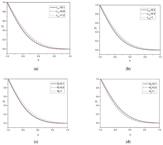
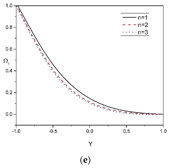
Figure 4.
(a–e): Solutal concentration 1 distribution versus Y for various physical parameters .
Figure 5a–e show the solutal concentration profile 2 of the nanoparticle is influenced by , , , , and . Figure 5a,b show that solutal concentration profile 2 in peristaltic motion increases by raising the values of and . Within the concentration boundary layer, both the solutal concentration 2 and Dofour solutal Lewis number are inversely proportional to the concentration difference at the wall. Therefore, the greater the Dofour solutal lewis number, the larger will be the solutal concentration 2. As a result of increased mass diffusivity, these parameters show a significant increase in solutal concentration profile 2 of the nanoparticle. Higher mass diffusivity indicates a higher possibility of molecular collision due to a large difference in solutal concentration. The difference in the solutal concentrations of molecules grows as the concentration gradient gets higher. Figure 5c demonstrates that solutal concentration profile 2 in peristaltic motion increases by rising the values of . Figure 5d shows a substantial decrease in solutal concentration profile 2 of the nanoparticle by enhancing the Brownian motion parameter . Brownian motion is based on a random motion of liquid elements moving across a flow surface as nanoparticle movement is pushed from the hot region to the cold region, which results in a decrease in the concentration distribution. Figure 5e presents the effect of the power-law index on the solutal concentration profile 2. The rise in power-law index decreases the solutal concentration profile 2 due to the reduced non-Newtonian behavior of the flow, and this leads to an enhancement of the momentum boundary layer.
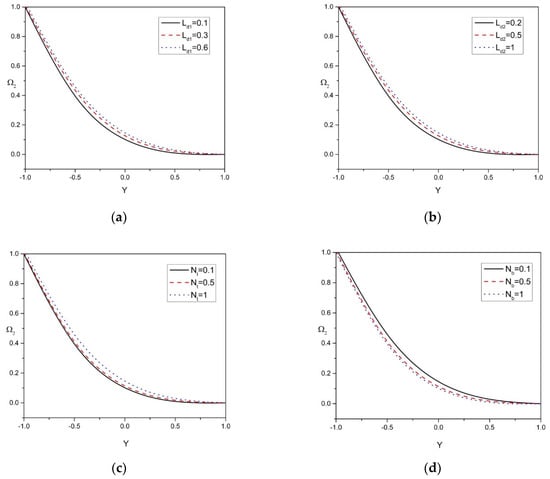
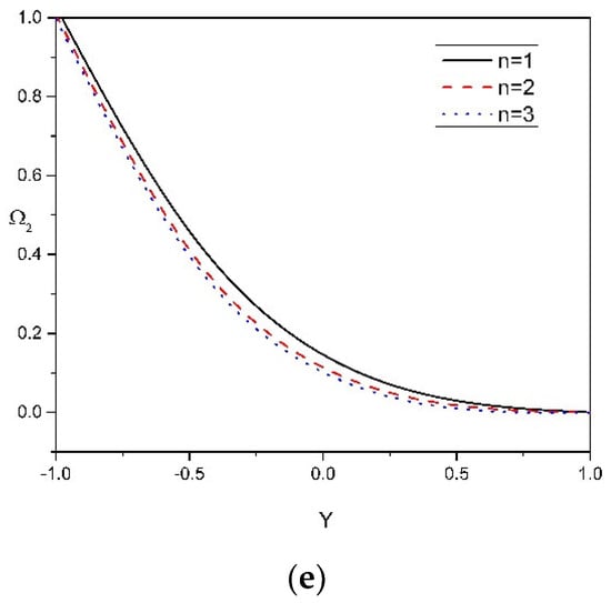
Figure 5.
(a–e): Solutal concentration 2 distribution versus Y for various physical parameters .
Figure 6a–e show that the solutal concentration profile of the nanoparticle are influenced by , , , , and . Figure 6a,b shows that the solutal concentration profile in peristaltic motion increases by raising the values of and . Within the concentration boundary layer, both the solutal concentration and Dofour solutal Lewis number are inversely proportional to the concentration difference at the wall. Therefore, the greater the Dofour solutal Lewis number, the larger will be the solutal concentration. As a result of increased mass diffusivity, these parameters show a significant increase in the solutal concentration profile of the nanoparticle. Higher mass diffusivity indicates a higher possibility of molecular collision due to a large difference in solutal concentration. The difference in the solutal concentrations of molecules grows as the concentration gradient gets higher. Figure 6c demonstrates that the solutal concentration profile in peristaltic motion increases by rising the values of . Figure 6d shows a substantial decrease in the solutal concentration profile of the nanoparticle by enhancing the Brownian motion parameter . Brownian motion is based on a random motion of liquid elements moving across a flow surface as nanoparticle movement is pushed from the hot region to the cold region, which results in a decrease in concentration distribution. Figure 6e presents the effect of the power-law index on the solutal concentration profile: a rise in the power-law index decreases the solutal concentration profile due to the reduced non-Newtonian behavior of the flow, and this leads to an enhancement of the momentum boundary layer.
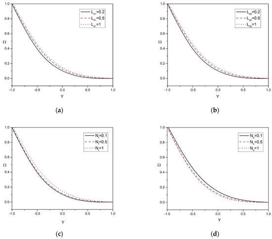
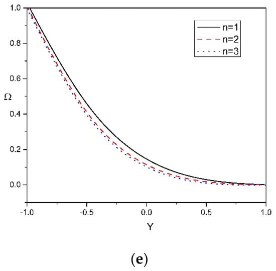
Figure 6.
(a–e): Solutal concentration distribution versus Y for various physical parameters .
4. Conclusions
This study reports the influence of natural convection with triple diffusion on peristaltic pumping under the assumptions of low Reynolds number and long wavelength of a Carreau nanoliquid in an asymmetric channel. Using graphs flow, the behavior of characteristics are examined.
The key findings of this article are as follows:
- ➢
- Velocity in peristaltic pumping decreases with an increase in . It grows with the thickness of the fluid, and that is why the velocity of the fluid depreciates. The influence of the power-law index on the velocity profile is also observed; it reduces the non-Newtonian behavior of the flow, and this leads to an enhancement of the momentum boundary layer.
- ➢
- It is observed that the velocity in peristaltic pumping rises with an increase in and due to the buoyancy force, which dominates within the boundary layer.
- ➢
- It is observed that the distribution of temperature increases for the larger varying values of modified Dufour parameters and .
- ➢
- It is noticed that temperature distribution increases for the larger varying values of Dufour solutal Lewis numbers and . In addition, the rise in power-law index decreases the temperature distribution due to the reduced non-Newtonian behavior of the flow, and this leads to an enhancement of the momentum boundary layer.
- ➢
- Solutal concentration 1, solutal concentration 2, and concentration of the nanoparticle in peristaltic pumping increase by raising the values of Dufour solutal Lewis parameters and . As a result of increased mass diffusivity, these parameters show a significant increase in solutal concentration 1, solutal concentration 2, and concentration of the nanoparticles.
- ➢
- The rise in power-law index also decreases the solutal concentration 1, solutal concentration 2, and concentration of the nanoparticles in peristaltic pumping due to the reduced non-Newtonian behavior of the flow, and this leads to an enhancement of the momentum boundary layer.
- ➢
- The differential transformation method (DTM) can be applied directly to nonlinear differential equations without requiring linearization and discretization, and therefore, it is not affected by errors associated with discretization. Unlike other methods, DTM is independent of any small or large quantities. Therefore, DTM can be applied whether or not governing equations and boundary/initial conditions of a given nonlinear problem contain small or large quantities.
- ➢
- Unlike the homotopy analysis method (HAM), DTM does not need to calculate auxiliary parameter Z1 through h-curves. DTM does not need initial guesses or an auxiliary linear operator, and it solves equations directly.
Author Contributions
Conceptualization, A.S.K. and J.B.; methodology, A.S.K. and J.B.; formal analyses, I.A.B., S.K., and N.A.A.; data curation, J.B., I.A.B., S.K., and N.A.A.; investigation, A.S.K. and J.B.; writing—original draft, A.S.K. and J.B.; resources, I.A.B., S.K., and N.A.A.; supervision A.S.K., project administration, A.S.K., I.A.B., S.K., and N.A.A.; review and editing, I.A.B., S.K., and N.A.A.; funding, A.S.K., I.A.B., and S.K. All authors have read and agreed to the published version of the manuscript.
Funding
King Khalid University (grant number R.G.P.2/63/43), Karnatak University Dharwad (Seed grant for research program KU/PMEB/2021/77).
Institutional Review Board Statement
Not applicable.
Informed Consent Statement
Not applicable.
Data Availability Statement
All data is available in the paper itself.
Acknowledgments
The authors extend their appreciation to the Deanship of Scientific Research at King Khalid University for funding this work through the research groups program under grant number R.G.P.2/63/43. Author A.S.K. is thankful to the Karnatak University, Dharwad, for their financial support under Seed grant for research program KU/PMEB/2021/77 (dated 25 June 2021). Author Joonabi Beleri would like to thank Directorate of Minorities for their financial support (DOMWDD/Ph.D//FELLOWSHIP/CR-01/2019-20). Date: 15 October 2019.
Conflicts of Interest
The authors declare no conflict of interest.
Nomenclature
| Cartesian coordinates | |
| Fluid mean temperature | |
| Temperature of the fluid | |
| Concentration of fluid | |
| Reynolds number | |
| Prandtl number | |
| Pressure of fluid | |
| Brinkman number | |
| Eckert number | |
| wave number | |
| Amplitude ratio | |
| Weissenberg number | |
| Base fluid’s density | |
| Density of particle | |
| Thermal conductivity | |
| Coefficient of Brownian diffusion | |
| Solutal diffusivity | |
| Coefficient of thermophoresis diffusion | |
| , , | Extra stress tensor components |
| and | Dufour and Soret type diffusivity |
| Volumetric thermal expansion coefficient | |
| , | Volumetric solutal expansion coefficients |
References
- Ghalambaz, M.; Moattar, F.; Sheremet, M.A.; Pop, I. Triple-diffusive natural convection in a square porous cavity. Transp. Porous Media 2016, 111, 59–79. [Google Scholar] [CrossRef]
- Archana, M.; Gireesha, B.J.; Prasanna Kumara, B.C. Triple diffusive flow of Casson nanofluid with buoyancy forces and nonlinear thermal radiation over a horizontal plate. Arch. Thermodyn. 2019, 40, 49–69. [Google Scholar] [CrossRef]
- Khan, W.A. Triple diffusion along a horizontal plate in a porous medium with convective boundary condition. Int. J. Therm. Sci. 2014, 86, 60–67. [Google Scholar] [CrossRef]
- Khan, Z.H. Triple convective-diffusion boundary layer along a vertical flat plate in a porous medium saturated by a water-based nanofluid. Int. J. Therm. Sci. 2015, 90, 53–61. [Google Scholar] [CrossRef]
- Umavathi, J.C.; Anwar Bég, O. Mathematical Modelling of Triple Diffusion in Natural Convection Flow in a Vertical Duct with Robin Boundary Conditions, Viscous Heating, and Chemical Reaction Effects. J. Eng. Thermophys. 2020, 29, 348–373. [Google Scholar] [CrossRef]
- Nawaz, M.; Awais, M. Triple diffusion of species in fluid regime using tangent hyperbolic rheology. J. Therm. Anal. Calorim. 2021, 146, 775–785. [Google Scholar] [CrossRef]
- Latham, T.W. Fluid Motion in a Peristaltic Pump. Master’s Thesis, Massachusetts Institute of Technology—MIT, Cambridge, MA, USA, 1966. [Google Scholar]
- Shapiro, A.H.; Jaffrin, M.Y.; Weinberg, S.L. Peristaltic pumping with long wavelengths at low Reynolds number. J. Fluid Mech. 1969, 37, 799–825. [Google Scholar] [CrossRef]
- Jaffrin, M.Y.; Shapiro, A.H. Peristaltic pumping. Annu. Rev. Fluid Mech. 1971, 3, 13–37. [Google Scholar] [CrossRef]
- Vajravelu, K.; Sreenadh, S.; Saravana, R. Combined influence of velocity slip, temperature and concentration jump conditions on MHD peristaltic transport of a Carreau fluid in a non-uniform channel. Appl. Math. Comput. 2013, 225, 656–676. [Google Scholar] [CrossRef]
- Reddy, R.H.; Kavitha, A.; Sreenadh, S.; Saravana, R. Effect of induced magnetic field on peristaltic transport of a Carreau fluid in an inclined channel filled with porous material. Int. J. Mech. Mater. Eng. 2011, 6, 240–249. [Google Scholar]
- Hayat, T.; Saleem, N.; Ali, N. Effect of induced magnetic field on peristaltic transport of a Carreau fluid. Commun. Nonlinear Sci. Numer. Simul. 2010, 15, 2407–2423. [Google Scholar] [CrossRef]
- Nadeem, S.; Akram, S.; Hayat, T.; Hendi, A.A. Peristaltic flow of a Carreau fluid in a rectangular duct. J. Fluids Eng. 2012, 134, 041201. [Google Scholar] [CrossRef]
- Choi, S.U.S. Enhancing Thermal Conductivity of Fluid with Nanoparticles. ASME Fluids Eng. Div. 1995, 231, 99–105. [Google Scholar]
- Asha, S.K.; Beleri, J. Peristaltic flow of Carreau nanofluid in presence of Joule heat effect in an inclined asymmetric channel by multi-step differential transformation method. World Sci. News 2022, 164, 44–63. [Google Scholar]
- Eldabe, N.T.; Abo-Seida, O.M.; Abo-Seliem, A.A.; ElShekhipy, A.A.; Hegazy, N. Peristaltic transport of magnetohydrodynamic Carreau nanofluid with heat and mass transfer inside asymmetric channel. Am. J. Comput. Math. 2017, 23, 74866. [Google Scholar] [CrossRef][Green Version]
- Machireddy, G.R.; Naramgari, S. Heat and mass transfer in radiative MHD Carreau fluid with cross diffusion. Ain Shams Eng. J. 2018, 9, 1189–1204. [Google Scholar] [CrossRef]
- Akram, S. Effects of nanofluid on peristaltic flow of a Carreau fluid model in an inclined magnetic field. Heat Transf.—Asian Res. 2014, 43, 368–383. [Google Scholar] [CrossRef]
- Zhou, J.K. Differential Transformation and Its Applications for Electrical Circuits; Huazhong University Press: Wuhan, China, 1986; pp. 1279–1289. [Google Scholar]
- Odibat, Z.M.; Bertelle, C.; Aziz-Alaoui, M.A.; Duchamp, G.H. A multi-step differential transform method and application to non-chaotic or chaotic systems. Comput. Math. Appl. 2010, 59, 1462–1472. [Google Scholar] [CrossRef]
- Hasona, W.M.; El-Shekhipy, A.; Ibrahim, M.G. Semi-analytical solution to MHD peristaltic flow of a Jeffrey fluid in presence of Joule heat effect by using multi-step differential transform method. New Trends Math. Sci. 2019, 7, 123–137. [Google Scholar] [CrossRef]
- Hasona, W.M. Temperature-dependent electrical conductivity and thermal radiation effects on MHD peristaltic motion of Williamson nanofluids in a tapered asymmetric channel. J. Mech. 2020, 36, 103–118. [Google Scholar] [CrossRef]
- Hasona, W.M.; El-Shekhipy, A.A.; Ibrahim, M.G. Combined effects of magnetohydrodynamic and temperature dependent viscosity on peristaltic flow of Jeffrey nanofluid through a porous medium: Applications to oil refinement. Int. J. Heat Mass Transf. 2018, 126, 700–714. [Google Scholar] [CrossRef]
- Tripathi, D.; Bég, O.A.; Gupta, P.K.; Radhakrishnamacharya, G.; Mazumdar, J. DTM simulation of peristaltic viscoelastic biofluid flow in asymmetric porous media: A digestive transport model. J. Bionic Eng. 2015, 12, 643–655. [Google Scholar] [CrossRef]
- Hatami, M.; Ghasemi, S.E.; Sahebi, S.A.R.; Mosayebidorcheh, S.; Ganji, D.D.; Hatami, J. Investigation of third-grade non-Newtonian blood flow in arteries under periodic body acceleration using multi-step differential transformation method. Appl. Math. Mech. 2015, 36, 1449–1458. [Google Scholar] [CrossRef]
- Bég, O.A.; Keimanesh, M.; Rashidi, M.M.; Davoodi, M.; Branch, S.T. Multi-step DTM simulation of magneto-peristaltic flow of a conducting Williamson viscoelastic fluid. Int. J. Appl. Math. Mech. 2013, 9, 1–19. [Google Scholar]
Publisher’s Note: MDPI stays neutral with regard to jurisdictional claims in published maps and institutional affiliations. |
© 2022 by the authors. Licensee MDPI, Basel, Switzerland. This article is an open access article distributed under the terms and conditions of the Creative Commons Attribution (CC BY) license (https://creativecommons.org/licenses/by/4.0/).