Usage of Selected Swarm Intelligence Algorithms for Piecewise Linearization

Abstract

The paper introduces a new approach to enhance optimization algorithms when solving the piecewise linearization problem of a given function. Eight swarm intelligence algorithms were selected to be experimentally compared. The problem is represented by the calculation of the distance between the original function and the estimation from the piecewise linear function. Here, the piecewise linearization of 2D functions is studied. Each of the employed swarm intelligence algorithms is enhanced by a newly proposed automatic detection of the number of piecewise linear parts that determine the discretization points to calculate the distance between the original and piecewise linear function. The original algorithms and their enhanced variants are compared on several examples of piecewise linearization problems. The results show that the enhanced approach performs sufficiently better when it creates a very promising approximation of functions. Moreover, the degree of precision is slightly decreased by the focus on the speed of the optimization process.

1. Introduction

Linearization is one of the most powerful methods that deal with nonlinear systems. One of the most important factors in piecewise linearization is the number of linear segments. Piecewise linear functions are often used to approximate nonlinear functions, and the approximation itself is an important tool for many applications. This method can be found in many applications, for example, dynamical systems, nonlinear non-smooth optimization, nonlinear differential equations, fuzzy ordinary differential equations and partial differential equations, petroleum engineering, and medicine [1,2,3,4,5].

Various existing approaches attempt to find a piecewise linear approximation of a given function. Classical mathematical methods based on differentiable nonlinear functions have been introduced, for example, the Newton–Kantorovich iterative method, analytical linearization, forward–difference approximation, or center-difference approximation [6,7]. Other types of classical transforms or approximations, e.g., Laplace, Fourier, or integral, are used for the construction of approximation models [8]. Methods based on fuzzy theory are called fuzzy approximation methods, and the most known method is called a fuzzy transform [9].

In [10], the authors introduced linearization methods that used the large deviation principle, utilizing the Donsker–Varadhan entropy of a Gaussian measure and the relative entropy of two probability measures. In [1], the author presented an easy and general method for constructing and solving linearization problems. A spline algorithm to construct the approximant and the interior point method to solve the linearization problem was created. In [11], the Wiener models were composed of a linear dynamical system together with a nonlinear static part. If the nonlinear part is invertible, the inverse function is approximated by a piecewise linear function estimated by the usage of the genetic algorithm and evolution strategy. The linear dynamic system part is estimated by the least square method.

In [12], the authors introduced a method to find the best piecewise linearization of nonlinear functions based on an optimization problem that is reduced to linear programming. Another algorithm that is used to find the optimal piecewise linearization for a predefined number of linear segments with particle swarm optimization (PSO), without the knowledge of the function and without ideal partitions, is introduced in [13]. Further, the authors of [14] introduced a genetic algorithm-based clustering approach to obtain the minimal piecewise linear approximation applied on nonlinear functions. The technique uses a trade-off between higher approximation accuracy and low complexity of the approximation by the least number of linearized sectors. Another piecewise linearization based on PSO is applied to piecewise area division; the control parameter optimization of the model was introduced in [15]. In [16], an effective algorithm to solve the stochastic resource allocation problem that designs piecewise linear and concave approximations of the recourse function of sample gradient information was introduced. In [17], the authors presented a range of piecewise linear models and algorithms that provided an approximation that fits well in their applications. The models involve piecewise linear functions using a constant maximum number of linear segments, border envelopes, strategies for continuity, and a generalization of the used models for stochastic functions.

We can already find some piecewise linearization problems solved by evolutionary algorithms, where specific kinds of functions or the number of piecewise linear parts are required. In this experiment, a kind of function is not restricted, and the number of linear segments does not need to be predefined. Nevertheless, only the 2D functions are used to be approximated in this experiment. Besides evolutionary algorithms, the traditional mathematical approaches were mentioned in this section to solve the piecewise linearization problems, however, these approaches will not be addressed in this paper, and a comparison with our methods will be mentioned in future work.

The aim of this paper is to contribute to the problem of piecewise linearization using popular swarm intelligence algorithms with automatic parameters tuning. The linearization of a given nonlinear function is an approximation problem leading to the determination of appropriate points. The goal is to find the best distribution of the points to minimize the distance between the original function and the approximated piecewise linear function. As there is no acceptable analytical solution of this optimization problem, using the stochastic-based (swarm intelligence) algorithms promises sufficient accuracy. Moreover, the selected swarm intelligence algorithms will be enhanced by the automatic parameter tuning approach and compared to provide an insight into the algorithm’s performance.

The rest of the paper is arranged as follows. In Section 2, the basic terms used in this paper are introduced. In Section 3, swarm intelligence algorithms selected for the comparison are briefly described. In Section 4, the application of the original swarm intelligence algorithms on piecewise linearization with their parameters is proposed. Finally, in Section 5, the application of the newly proposed automatic parameter tuning of the swarm intelligence algorithms is introduced. A compendious discussion of the algorithm’s efficiency and precision is assumed in Section 6.

2. Preliminaries

In this paper, we work with a real-value problem in a continuous search area. We consider the objective function $f\left(x\right)$, where $x=(x_1,x_2,\dots ,x_{\ell })$, $\ell \in \mathbb{N}$ is defined on the search domain $X=[a,b]$. The problems solved in a discrete search space could require some modifications of the presented methods. Through this paper, for the simplicity of the demonstrated method, the domain $[0,1]$ is used, but the problem can be easily reduced to the more general domain.

2.1. Piecewise Linear Function

Through this paper, piecewise linear functions are used, therefore the piecewise linear function should be defined.

A piecewise linear function $f:[0,1]\to [0,1]$ given by finite number of points $(x_i,y_i)\in [0,1]\times [0,1]$ for $i=1,\dots ,\ell$, is a function $f:[0,1]\to [0,1]$ such that $x_1=0,x_{\ell }=1$, and $f\left(x_i\right)=y_i$ for each $i=1,2,\dots ,\ell$, and ${f|}_{[x_i,x_i+1]}$ is linear for every $i=1,2,\dots ,\ell -1$. Points x are called turning points. More precisely,

$$f\left(x\right)=\left\{\begin{array}{cc}{y}_1+(y_2-y_1)\frac{(x-x_1)}{(x_2-x_1)},\hfill & x_1\le x\le x_2,\hfill \\ y_2+(y_3-y_2)\frac{(x-x_2)}{(x_3-x_2)},\hfill & x_2\le x\le x_3,\hfill \\ ⋮\hfill \\ y_{\ell -1}+(y_{\ell }-y_{\ell -1})\frac{(x-x_{\ell -1})}{(x_l-x_{\ell -1})},\hfill & x_{\ell -1}\le x\le x_{\ell }.\hfill \end{array}\right.$$

2.2. Metrics

The difference between the original function and the approximated piecewise linear function is calculated with chosen metrics. In this paper, two different metrics are applied to achieve more complex results of compared methods.

Let $(\mathbf{x},\mathbf{y})$ are vectors, where $\mathbf{x}=\{x_1,x_2,\dots ,x_n\}$, $\mathbf{y}=\{y_1,y_2,\dots ,y_n\}$. A Manhattan metric is a function $d_1:{\mathbb{R}}^n\times {\mathbb{R}}^n\to \mathbb{R}$ in n-dimensional space, which gives the distance between vectors $\mathbf{x},\mathbf{y}$ by the sum of the line segments projection lengths between the points onto the coordinate system. More precisely,

$$d_1(\mathbf{x},\mathbf{y})=\sum _{i=1}^n|{\mathbf{x}}_{\mathbf{i}}-{\mathbf{y}}_{\mathbf{i}}|.$$

A metric defined on a vector space, induced by the supremum or uniform norm, where the two vectors distance is the biggest of the differences, is called Maximum metric. More precisely,

$$d_2(\mathbf{x},\mathbf{y})=\underset{\mathbf{i}=\mathbf{1},\mathbf{2},\dots ,\mathbf{n}}{max}|{\mathbf{x}}_{\mathbf{i}}-{\mathbf{y}}_{\mathbf{i}}|.$$

3. Selected Swarm Intelligence Algorithms

Now, the use of swarm algorithms for searching a global optima of an interval map $f:[0,1]\to [0,1]$ will be demonstrated. A population is represented as a finite set of $n\in \mathbb{N}$ randomly chosen points $x\in [0,1]$. Further, the population moves in the domain with the help of the given algorithm strategy. The processes are mostly combined with the help of stochastic parameters, adapted towards the required solution. These algorithms stop after a certain number of iterations or under some predefined condition. The algorithms were selected based on the popularity of the methods measured by the frequency of their real applications and also based on our previous experiments [18,19].

3.1. Swarm Intelligence Algorithms

Swarm intelligence algorithms are stochastic algorithms from the group of evolutionary algorithms. These algorithms are used for solving global optimization problems that model the social behaviors of a group of individuals. The inspiration comes mostly from nature, especially from biological systems inspired by biological evolution, such as selection, crossover, and mutation. Most swarm intelligence in nature-based systems involve algorithms of ant colonies, bird flocking, hawk hunting, animal herding, fish schooling, and others. The difference between evolutionary algorithms and swarm intelligence is that there is an interaction of more candidate solutions, but they differ in the model between individuals. In swarm intelligence algorithms, there is also a group (population), but its move in the domain is followed by the group behavior rules of a given population. In this section, the swarm algorithms used in this manuscript will be introduced.

3.1.1. Particle Swarm Optimization

A population in the PSO algorithm is composed of particles that move in a predefined search area according to evolutionary processes. In each step, several characteristics are computed and employed to illustrate how the particles are toward the solution [20,21,22].

The population is represented by a finite set of $n\in \mathbb{N}$ points $x\in [0,1]$ called particles is given randomly. Then, the population is evaluated, and each particle controls its movement in the search area according to its personal best position $p_{best}$, the best neighbour position ${\mathbf{p}}_g$ and with the stochastic parameters (acceleration coefficients ${\Phi }_1,{\Phi }_2$, constriction factor $\chi$). There exist several variants of the PSO algorithm. In this paper, the original PSO algorithm from [21] with the modification by constriction factor $\chi$ is used. Parameter $\chi$ does not change during the algorithm’s run and it has a restrictive impact on the result. When the PSO algorithm runs without restraining velocities, it can rapidly increase to unacceptable levels within a few iterations. The elements $U_{{\Phi }_1}$, $U_{{\Phi }_2}$ are represented by random points from a uniformly distributed intervals $[0,{\Phi }_1]$, $[0,{\Phi }_2]$, where ${\Phi }_1,{\Phi }_2\in \mathbb{R}$. At first, $p_{bes{t}_i}$ and $f\left({\mathbf{x}}_i\right)$ are compared, and if $p_{bes{t}_i}\le f\left({\mathbf{x}}_i\right)$, then ${\mathbf{p}}_i={\mathbf{x}}_i$ and to the value of $p_{bes{t}_i}$ is saved a value of the function ($p_{bes{t}_i}=f\left({\mathbf{p}}_i\right)$). In the next step, it finds the best neighbour ${\mathbf{p}}_g$ of i-th position and assign it j-th position, if $f\left({\mathbf{p}}_g\right)\ge f\left({\mathbf{x}}_j\right)$, then ${\mathbf{p}}_g={\mathbf{x}}_j$ and $f\left({\mathbf{p}}_g\right)=f\left({\mathbf{x}}_j\right)$. The main part of the calculation consists of computing the velocity and updating the new particle positions which are given by the following formulas:

$${\mathbf{v}}_i=\chi ({\mathbf{v}}_i+{\mathbf{U}}_{{\Phi }_1}({\mathbf{p}}_i-{\mathbf{x}}_i)+{\mathbf{U}}_{{\Phi }_2}({\mathbf{p}}_g-{\mathbf{x}}_i)),$$

$${\mathbf{x}}_i={\mathbf{x}}_i+{\mathbf{v}}_i.$$

3.1.2. Self-Organizing Migrating Algorithm

A self-organizing migrating algorithm (SOMA) is a simple model of the hunting pack. The individuals move across the domain, such that each individual in each migration round goes straight to the leader of the pack, checks the place of each jump, and remembers the best-found place for the next migration round. SOMA has several strategies, we use the’ AllToOne’ strategy, where all individuals move towards the best one from the population. Each individual $x_i\in [0,1]$ is evaluated by the fitness, and the one with the highest fitness is chosen as a leader for the loop. Then the rest of the individuals jump towards the leader and each of them is evaluated by the cost function after each jump. SOMA has three numerical parameters defining a way of moving an individual behind the leader. These parameters are the relative size of the skipping leader, the size of each jump, and the parameter which determines the direction of movement of the individual behind the leader. The jumping approach continues until a new individual-position restricted by $\mathit{PathLength}$ is reached. The new individual position at the end of each jump is determined by

$$x_i^{\mathit{ML}+\mathit{1}}=x_{i,start}^{\mathit{ML}}+(x_L^{ML}-x_{i,start}^{\mathit{ML}})\mathit{StepSize}·\mathit{PRTVector}.$$

Then each individual moves toward the best position on its jumping trajectory. Before an individual continues to jump towards the leader, a set of random numbers from the interval $[0,1]$ is generated, and each member of this set is compared with $\mathit{PRT}$, where $\mathit{PRT}\in [0,1]$. If the generated random number is greater than $\mathit{PRT}$, the corresponding ith coordinate will be taken from the new position (${\mathit{PRTVector}}_j=1$) otherwise it will be taken from the original individuals position (${\mathit{PRTVector}}_j=0$). During the process, each individual attempts to find its best position and the best position from all individuals [23].

3.1.3. Cuckoo Search

The Cuckoo search (CS) algorithm is inspired by brood parasitism of cuckoos which give eggs in the nests of the host birds. The host bird throws the egg away from the nest or abandons the nest whereas build a new nest by the fraction $p_a$. The idea of the algorithm is to create new and better solutions (cuckoos) that replace worse solutions from the nests. Each egg represents one solution and a cuckoo egg gives a new possible solution. In our case, we use the easiest form of the algorithm when each nest has one egg.

Cuckoo search uses the Mantegna Lévy flight $\mathit{L}é\mathit{vy}\left(\beta \right)$, which is given by the following equation: $step=u/{\left|v\right|}^{1/\beta }.$ The parameter $\beta$ is taken from the interval $[0.3,2)$, parameters $u,v$ are normally distributed stochastic variables and u is calculated as $u·\sigma$, where $\sigma$ is the standard deviation. The main part of the algorithm is the application of Lévy flights and random walks in the equation that generates new solutions:

$${\mathbf{x}}_i^{t+1}={\mathbf{x}}_i^t+\alpha \mathit{L}é\mathit{vy}\left(\beta \right).$$

The parameter $\alpha >0$ is the step size, and mostly, the value $\alpha =1$ can be used. The total number of possible host nests is constant, where the probability that the host bird discovers a cuckoo’s egg is $p_a\in [0,1]$ [24].

3.1.4. Firefly Algorithm

Firefly algorithm (FFL) is inspired by the flashing behavior of fireflies that produce light at night. Fireflies are unisexual; therefore, they are attracted to each other no matter their sex. A new generation of fireflies is given by the random walk and their attraction. Fireflies can communicate with their light intensity that informs the swarm about its features as species, location, and attractiveness. Between any two fireflies i and j the Euclidean distance $r(i,j)$ at positions ${\mathbf{x}}_i$ and ${\mathbf{x}}_j$ is defined. The attractiveness function of a firefly j should be selected as any monotonically decreasing function with a distance to the selected firefly defined as $\beta ={\beta }_0·e^{-\gamma ·r_{ij}^2}$, where $r_{ij}$ is the distance, ${\beta }_0$ is the initial attractiveness at a distance $r_{ij}=0$, and $\gamma$ represents an absorption coefficient characterizing the variation of the attractiveness value. The movement of each ith firefly attracted by a more firefly j with higher attractiveness is given by the equation

$${\mathbf{x}}_i^{t+1}={\mathbf{x}}_i^t+\beta ({\mathbf{x}}_j^t-{\mathbf{x}}_i^t)+\alpha (\sigma -0.5).$$

The first component represents the ith firefly position, the second part enables the model of the attractiveness of the firefly, and the last part is randomization, with $\alpha \in [0,1]$ represented by the problem of interest. The parameter $\sigma$ represents a scaling factor that determines the distance of visibility, and mostly $\sigma \in [0,1]$ that is given by a random uniform distribution in the space can be used [25].

3.1.5. Grey Wolf Optimizer

Grey wolf optimizer (GWO) is inspired by wolves living in a pack. In the mathematical model of the wolves’ social hierarchy, the best solution is represented by $\alpha$, the second-best solution is $\beta$, and $\delta$ represents the third-best solution. The rest of the candidate solutions are in a group $\omega$. The optimization in this algorithm is guided by the best three wolves $\alpha ,\beta ,\delta$, and the wolves in $\omega$ follow these three wolves. The model is given by the following equations:

$$\mathbf{d}=|\mathbf{c}·{\mathbf{x}}_P^{\left(t\right)}-{\mathbf{x}}^{\left(t\right)}|$$

and

$${\mathbf{x}}^{(t+1)}={\mathbf{x}}_p^{\left(t\right)}-\mathbf{a}·\mathbf{d},$$

where t is the current iteration, variables $\mathbf{a}$ and $\mathbf{c}$ are coefficient vectors, ${\mathbf{x}}_p$ is the prey’s position vector, and $\mathbf{x}$ represents the position vector of a grey wolf. The vectors $\mathbf{a}$ and $\mathbf{c}$ are determined as follows: $\mathbf{a}=2a{r}_1-a$, $\mathbf{c}=2r_2$. Components of $\mathbf{a}$ are linearly decreased from 2 to 0 over the course of iterations by the formula $2-(2\frac{\mathit{FES}}{\mathit{maxFES}}$), where $\mathit{maxFES}$ is a total count of fitness value evaluations, and $r_1,r_2$ are random values from interval $[0,1]$ [26].

3.1.6. Artificial Bee Colony

The artificial bee colony (ABC) is inspired by the foraging behavior of honey bees, and it employs three types of bees: employed foraging bees, onlookers, and food sources. Employed foraging bees and onlookers search for food sources, and for one food source equals to one employed bee. It means the number of employed bees is the same as the number of food places around the hive. The algorithm randomly places a population of initial vectors, which is iteratively improved. The possible solution is represented by the position of the food, and the food source gives the quality (fitness) of a given problem [27]. The ABC algorithm is quite simple because it uses only three control parameters that should be determined (size of the population, limit of scout L, dimension of the problem).

The new solution is given by the following formula

$${\mathbf{v}}_i={\mathbf{x}}_i+{\varphi }_i({\mathbf{x}}_i-{\mathbf{x}}_k),$$

where k and j are randomly selected indexes and $\varphi$ is random number from the range $[-1,1]$. Then, it computes the probability value p for the solutions x with the help of the fitness value. The next step is to produce and evaluate new onlookers solutions ${\mathbf{v}}_i$, which are based on the solutions ${\mathbf{x}}_i$ that depends on ${\mathbf{p}}_i$.

3.1.7. Bat-Inspired Algorithm

The inspiration of the bat-inspired algorithm (BIA) comes from the echolocation behavior of microbats, which use varying pulse rates controlled by emission and loudness. Each bat flies randomly with a given velocity, and it has its position with a varying frequency or wavelength and loudness. All bats use echolocation; thus, they know the distance and the difference between food.

The population of bats is placed randomly, and after that, they fly randomly with a given velocity ${\mathbf{v}}_i$ to the position ${\mathbf{x}}_i$ with a given frequency $f_{min}$, changing wavelength $\lambda$, and loudness parameter $A_0$. The bats automatically adjust the proper wavelength of the emitted pulses, and also the pulse emission rate $r\in [0,1]$. The loudness can vary, for example, between $A_0$ and a minimum value $A_{min}$. The frequency f is in a range $[f_{min},f_{max}]$ and it corresponds to the range of wavelengths $[{\lambda }_{min},{\lambda }_{max}]$. Here, the wavelengths are not used, instead, the frequency varies whereas the wavelength $\lambda$ is fixed. This is caused by the relation between $\lambda$ and f, where $\lambda ·f$ is constant. For simplicity, the frequency is set from $f\in [0,f_{max}]$. It is clear that higher frequencies give short wavelengths and provide a shorter distance. The rate of the pulse can be in the interval $[0,1]$, where 0 denotes no pulses, and 1 marks the maximum rate of pulse emission. The new solutions ${\mathbf{x}}_i^t$ and velocities ${\mathbf{v}}_i^t$ at current time t are given by

$$f_i=f_{min}+(f_{max}-f_{min})\beta ,$$

$${\mathbf{v}}_i^t={\mathbf{v}}_i^{t-1}+({\mathbf{x}}_i^t-{\mathbf{x}}_{best})f_i,$$

$${\mathbf{x}}_i^t={\mathbf{x}}_i^{t-1}+{\mathbf{v}}_i^t,$$

where $\beta \in [0,1]$ represents a uniformly distributed random vector, and value ${\mathbf{x}}_{best}$ demonstrates the current global best position detected after comparing all bat-solutions. The local search strategy generates a new solutions for each bat using random walk ${\mathbf{x}}_{new}={\mathbf{x}}_{old}+ϵ{\mathbf{A}}^t$, where $ϵ\in [-1,1]$ is a random number, while ${\mathbf{A}}^t=\left\{A_i^t\right\}$ is the mean loudness of whole bats population in the current time step. The loudness parameter ${\mathbf{A}}_i$ and the pulse emission rate $r_i$ are updated during the iterations proceed. Now we have $A_i^{t+1}=\alpha A_i^t$, $r_i^{t+1}=r_i^0[1-e^{-\gamma t}]$, where $\alpha$ and $\gamma$ are constants. For any $0<\alpha <1$ and $\gamma >0$, we have $A_i^t\to 0,r_i^t\to r_i^0$, as $t\to \infty$ [28].

3.1.8. Tree-Seed Algorithm

The tree-seed algorithm (TSA) is based on the relationship observed between trees and seeds, where seeds gradually grow, and new trees are created from them. The trees’ surface is represented by a search area, and the tree and seed locations are mentioned as possible solutions of the optimization problem. It employs two peculiar parameters as the total number of trees and the seed production. The main and important problem is to obtain the seed location produced from a tree. The first equation finds the tree location used for the production of the seed, whereas the second employs the locations of two different trees to produce a new seed for the tree:

$$s_{i,j}=t_{i,j}+{\alpha }_{i,j}\times (b_j-t_{r,j}),$$

$$s_{i,j}=t_{i,j}+{\alpha }_{i,j}\times (t_{i,j}-t_{r,j}),$$

where $s_{i,j}$ is jth dimension of ith seed position to produce ith tree and $t_{i,j}$ is the jth dimension of the ith tree, $b_j$ represents the jth dimension of the best tree, where b is computed as $b=min\left\{f\left(t_i\right)\right\}$, the jth dimension of rth tree $t_{r,j}$ is selected from the population randomly. The scaling factor $\alpha$ is produced randomly from $[-1,1]$, i and r are different indices.

First, the initial tree locations that give us trial solutions of the optimization problem are designed by using:

$$t_{i,j}=l_{j,min}+r_{i,j}(h_{j,max}-l_{j,min})$$

where, $l_{j,min}$ represents the lower bound of the search area, $h_{j,max}$ denotes the upper bound of the search area, and $r_{i,j}\in [0,1]$ is a uniformly distributed random number. The best solution is selected from the population using b where n represents the size of the trees population. The number of seeds can be higher than the number of trees [29].

3.1.9. Random Search

Random search (RS) is the simplest stochastic algorithm for global optimization, which was proposed by Rastrigin in 1963. In every iteration, it generates a new point from the uniform distribution in the search area. Then, the function value of this point is compared with the best point found so far. If the new trial point is better, it replaces the old best point. There is not used any learning mechanism or exploitation of knowledge from the previous search [30]. This algorithm does not belong to the group of swarm algorithms, but because it can have fast and good convergence to the given solution, it can be used as a comparing algorithm.

4. Piecewise Linearization Using Swarm Intelligence Algorithms

Our implementation of the swarm algorithms consists of searching for a linearization $l_f$ (the piecewise linear function definition is above) of a fixed interval map $f:[0,1]\to [0,1]$. To allocate a suitable solution, the optimization function (objective function) is represented by a distance function given by the metric between f and its linearization $l_f$. Every possible linearization is represented by a finite number of points ($\ell \in \mathbb{N}$), every population contains n particles (ℓ-dimensional vectors), where the stochastic parameters are adapted.

In this section, we introduce the testing functions, provide the setting of the algorithm’s parameters that can be used for the problem of linearization, and we look at which algorithm can give us the best results.

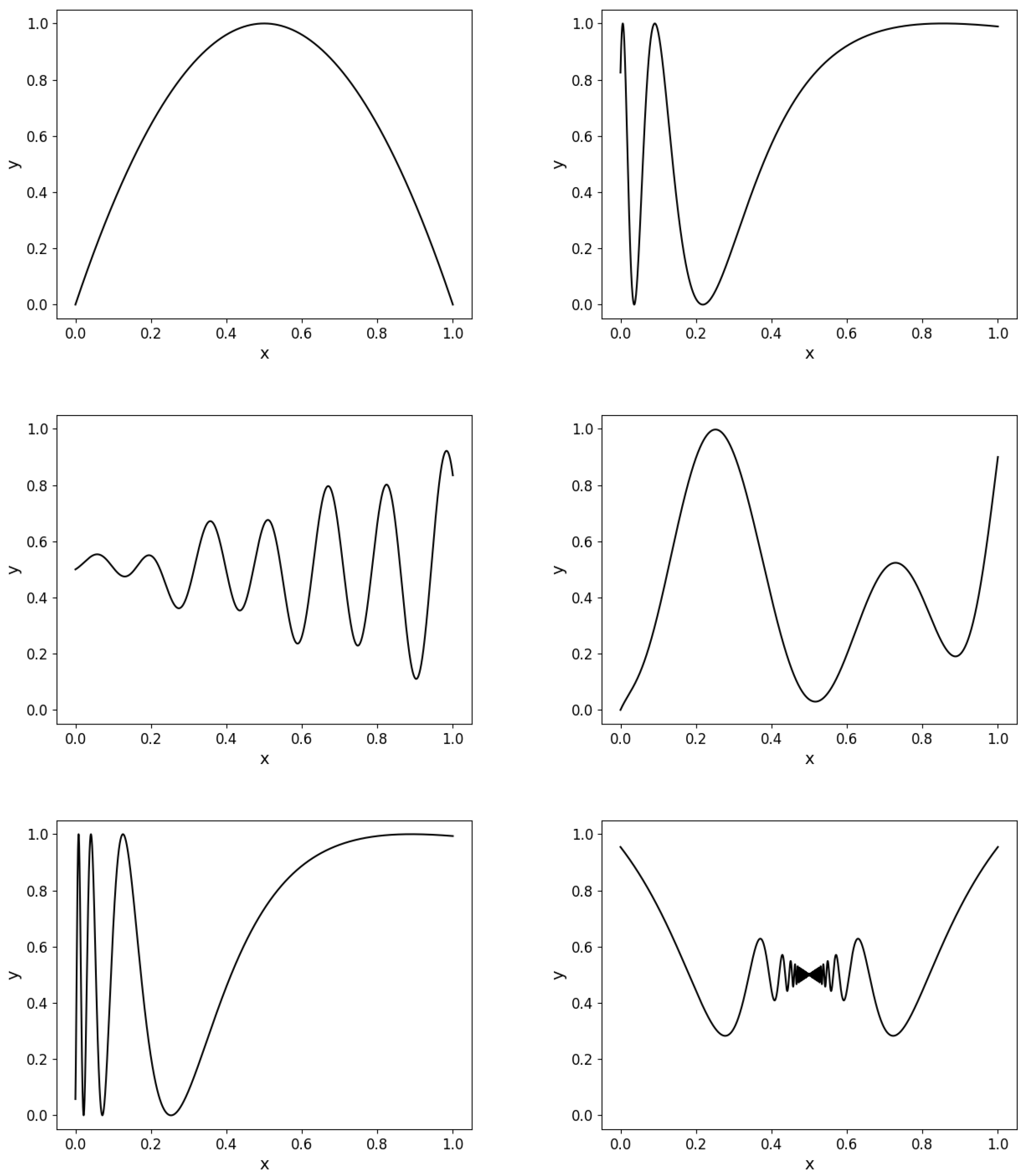
4.1. Test Functions

For testing, we chose continuous functions $f:[0,1]\to [0,1]$, where for simplicity, we work only in the space $[0,1]$. These functions were chosen from the most basic to the complicated ones (see Figure 1), to demonstrate the algorithm behavior on different levels of functions. The functions are given by the following formulas:

$$f_1\left(x\right)=4x-4x^2$$

(1)

$$f_2\left(x\right)=\frac{1}{2}(sin(\frac{\frac{3}{2}}{x+\frac{1}{10}})+1)$$

(2)

$$f_3\left(x\right)=\frac{1}{25}(sin20x+20x·sin20x·cos20x)+\frac{1}{2}$$

(3)

$$\begin{array}{c}\hfill f_4\left(x\right)=0.9+(-1+x)(0.9+(-0.16+(5.4+(-27+\\ \hfill (36+(510+(-120-2560(-0.9+x\left)\right)(-0.1+x))\\ \hfill (-0.6+x)\left)\right(-0.2+x\left)\right)(-0.8+x)\left)\right(-0.4+x\left)\right)x)\end{array}$$

(4)

$$f_5\left(x\right)=sin\left(\frac{\frac{3}{2}}{x+\frac{13}{200}}\right)+1$$

(5)

$$f_6\left(x\right)=(x-\frac{1}{2})sin\left(\frac{1}{x-\frac{1}{2}}\right)+\frac{1}{2}$$

(6)

4.2. Parameter Settings of the Chosen Algorithms

The proper choice of parameters can have a large influence on the optimization performance and, therefore, for each algorithm, in comparison, we tested which parameters were suitable for our problem, in regard to searching for the best possible linearization. In this subsection, we will discuss the setting of parameters for the algorithms introduced in Section 3.1. Each algorithm proceeded 50 times with a fixed dimension $\ell =16$ and also a fixed population size set to $n=25$. Each algorithm runs as long as it takes to find a solution with a good enough $fitness\_value$, but it has to find it before $\mathit{maxFES}=$ 10,000. This $\mathit{fitness}\_\mathit{value}$ threshold was set to value $0.2$.

In PSO, the setting of acceleration coefficients ${\Phi }_1,{\Phi }_2$ and constriction factor $\chi$ should be set. Parameter ${\Phi }_1$ controls the importance of the particle’s personal best value, whereas the importance of the neighbor best value is controlled by parameter ${\Phi }_2$. The algorithm can be unstable when these parameters are too high because the velocity can grow up faster. The equation $\Phi ={\Phi }_1+{\Phi }_2$, where $\Phi >4$, should be satisfied and the authors of the algorithm recommended ${\Phi }_1,{\Phi }_2$ set to $2.05$. Parameter $\chi$ has a restrictive effect on the result, and it does not change in time. In the original version, PSO has $\chi =\frac{2}{\left(\Phi -2+\sqrt{{\Phi }^2-4\Phi }\right)}$.

In SOMA, there are a few parameters in which the settings should be considered and tested. Parameter $PathLength\in (1,5]$ is a parameter that defines how far an individual stops behind the leader. The StepSize is from the interval $(0,PathLength]$ and step is from the interval $(0,1]$. One of the most sensitive parameters is $\mathit{PRT}\in [0,1]$, which represents the perturbation and decides if an individual will travel towards the leader directly or not [23].

In the original version of the cuckoo search algorithm, parameter $\beta$ is taken from the interval $[0.3,2)$. The step size $\alpha >0$ is dependent on the scales of the problem, and mostly, the value $\alpha =1$ is used. The total number of possible host nests is restricted, where the probability that the host bird discovers a cuckoo’s egg is $p_a\in [0,1]$.

In the firefly algorithm, the parameter ${\beta }_0=1$ is the initial attractiveness for a distance $r_{ij}=0$. Parameter of $\gamma$ represents an absorption coefficient that characterizes the variation of the attractiveness value of a firefly. If ${\beta }_0=0$, it becomes a simple random walk.

All parameters used in the grey wolf optimizer are given by random values, so there is no need for more detailed parameter testing.

The control parameters in the ABC algorithm, which should be set, are the size of the population $CS$ and the limit for scout ($L=\frac{(CS·D)}{2}$, where D is the dimension of the problem).

In the original version of the bat-inspired algorithm, the values $f_{min}=0$ and $f_{max}=100$ depends on the size of the search area dimension. Each bat has a randomly assigned frequency with the uniform distribution of $[f_{min},f_{max}]$. For simplicity, it can be used $\alpha =\gamma$, and in the original version author used $\alpha =\gamma =0.9$, but for our case, we had to do experimental testing. For each bat individual, different values of loudness and pulse emission rate are recommended, based on randomization. In the tree-seed algorithm, importance is given to the selection of an equation that will produce a new seed location. Control parameter $ST\in [0,1]$, called search tendency, is used for the selection. The seed number of each tree is determined randomly, and it should not be less than 1. The recommended number of randomly generated seeds is between 10 and 25% of the number of trees.

For a better overview of the algorithm configuration, the settings of the numerical parameters are assumed in

Table 1. Parameters setting.

Algorithm	Parameter	Optimal Interval	Chosen Value
	$\chi$	-	0.69
PSO	${\varphi }_1$	-	2.45
	${\varphi }_2$	-	1.65
	$step$	$[0.11,0.31]$	0.11
SOMA	PathLength	$[3.5,5.0]$	4.7
	PRT	$[0.6,0.9]$	0.6
CS	$p_a$	$[0.0,1.0]$	0.25
	${\beta }_0$	$[0.0,1.66]$	1.5
	$\alpha$	$[0.0,1.0]$	1.0
FFL	$\gamma$	$[7,10]$	10
	${\beta }_0$	$[0.6,1.0]$	0.8
ABC	L	-	50
BIA	$\alpha$	-	0.9
	$\gamma$	-	0.9
	$r_0$	$[0,0.2],[0.8,1.0]$	0.8
	$A_0$	$[1.0,1.6]$	1.6
	$l_{j,min}$	$[0.05,0.25]$	0.25
TSA	$h_{j,max}$	$[0.5,1.0]$	0.9
	$ST$	-	0.1

. The Optimal Interval column presents the intervals containing the achieved acceptable values of the parameters. In the Chosen Value column, the final values of the parameters are presented.

4.3. Examples of Piecewise Linearization

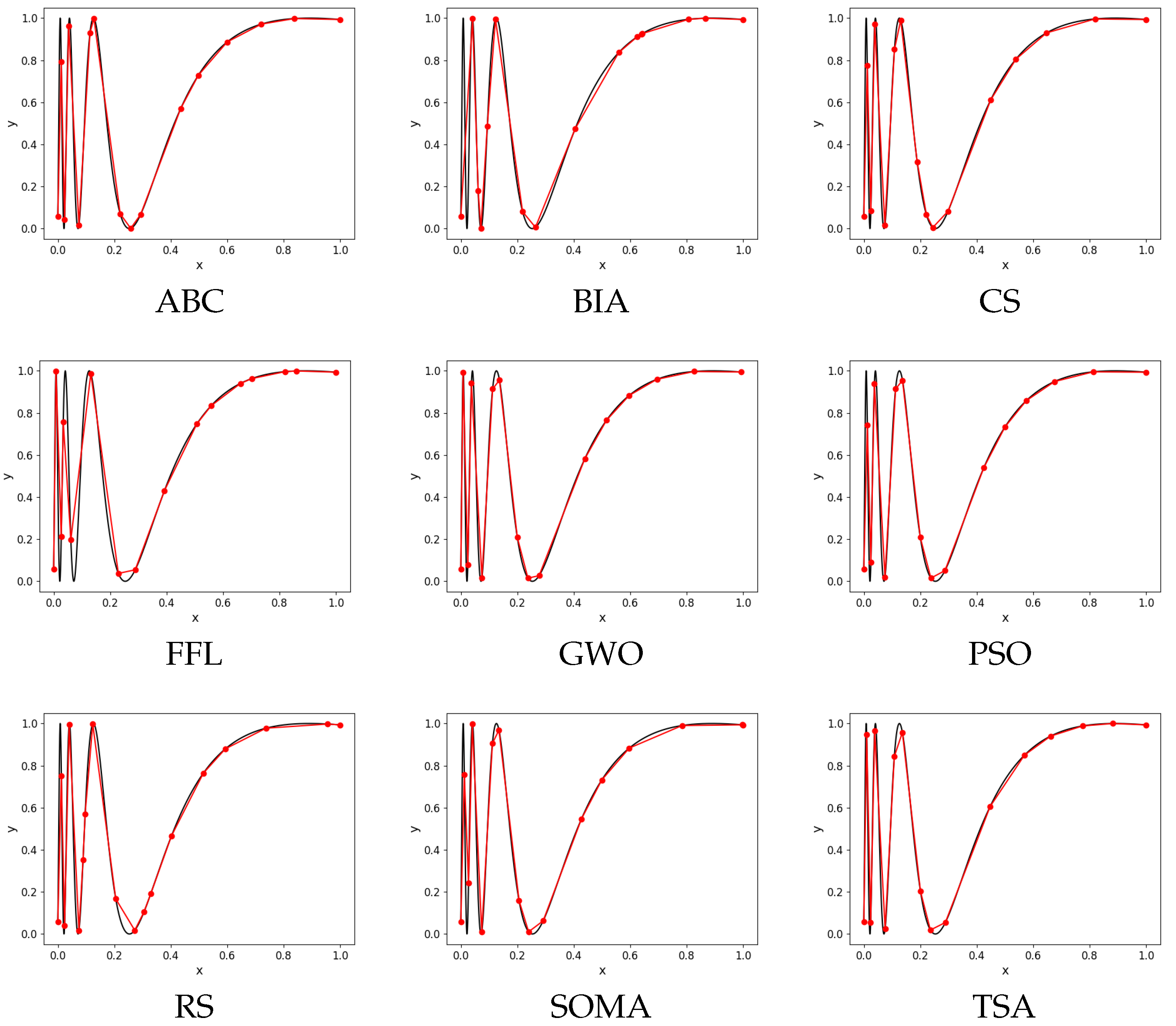
In this subsection, we will demonstrate an example of linearization for Function $f_5$ given by all chosen evolutionary algorithms. To demonstrate how the algorithm works, the graph of results for Function $f_5$ of each evolutionary algorithm is presented (Figure 2). Each evolutionary algorithm has set its input parameters in accordance with Section 4.2.

4.4. Summary of Results

In this subsection, we will introduce a set of tables showing the results of each evolutionary algorithm, and to make the results clearer, we chose to use only the four testing functions introduced in Section 4.1.

The following tables (

Table 2. Comparison of algorithms for Function $f_1$.

	Mean	Median	SD	Min	Max
PSO	0.206	0.204	0.007	0.202	0.235
SOMA	0.211	0.209	0.005	0.204	0.234
CS	0.202	0.202	0.001	0.202	0.203
FFL	0.284	0.283	0.013	0.252	0.313
GWO	0.223	0.220	0.018	0.199	0.264
ABC	0.203	0.203	0.004	0.191	0.212
BIA	0.430	0.431	0.059	0.329	0.567
TSA	0.214	0.212	0.004	0.204	0.227
RS	0.231	0.231	0.011	0.204	0.258

,

Table 3. Comparison of algorithms for Function $f_3$.

	Mean	Median	SD	Min	Max
PSO	2.388	2.283	0.353	1.931	3.656
SOMA	2.377	2.352	0.256	1.973	3.309
CS	2.524	2.533	0.180	2.152	3.116
FFL	5.245	5.269	0.267	4.594	5.742
GWO	3.575	3.304	0.718	2.908	5.649
ABC	2.088	2.079	0.079	1.908	2.256
BIA	6.014	6.093	0.621	4.509	6.935
TSA	2.453	2.440	0.203	2.137	2.951
RS	3.372	3.389	0.227	2.831	3.830

,

Table 4. Comparison of algorithms for Function $f_4$.

	Mean	Median	SD	Min	Max
PSO	0.847	0.828	0.062	0.783	1.112
SOMA	0.892	0.881	0.052	0.820	1.024
CS	0.863	0.854	0.039	0.803	0.983
FFL	2.180	2.206	0.184	1.707	2.523
GWO	1.824	1.808	0.143	1.524	2.347
ABC	0.822	0.820	0.017	0.789	0.895
BIA	2.320	2.230	0.354	1.831	3.447
TSA	0.912	0.914	0.044	0.832	1.032
RS	1.187	1.184	0.077	0.981	1.335

and

Table 5. Comparison of algorithms for Function $f_5$.

	Mean	Median	SD	Min	Max
PSO	1.719	1.705	0.321	0.890	3.066
SOMA	1.927	1.966	0.132	1.426	2.140
CS	1.662	1.704	0.187	1.143	2.067
FFL	3.347	3.400	0.251	2.625	3.772
GWO	2.174	2.023	0.291	1.886	2.705
ABC	1.632	1.688	0.220	1.112	1.977
BIA	3.726	3.771	0.419	2.501	4.351
TSA	1.718	1.729	0.146	1.149	1.959
RS	2.144	2.159	0.139	1.499	2.383

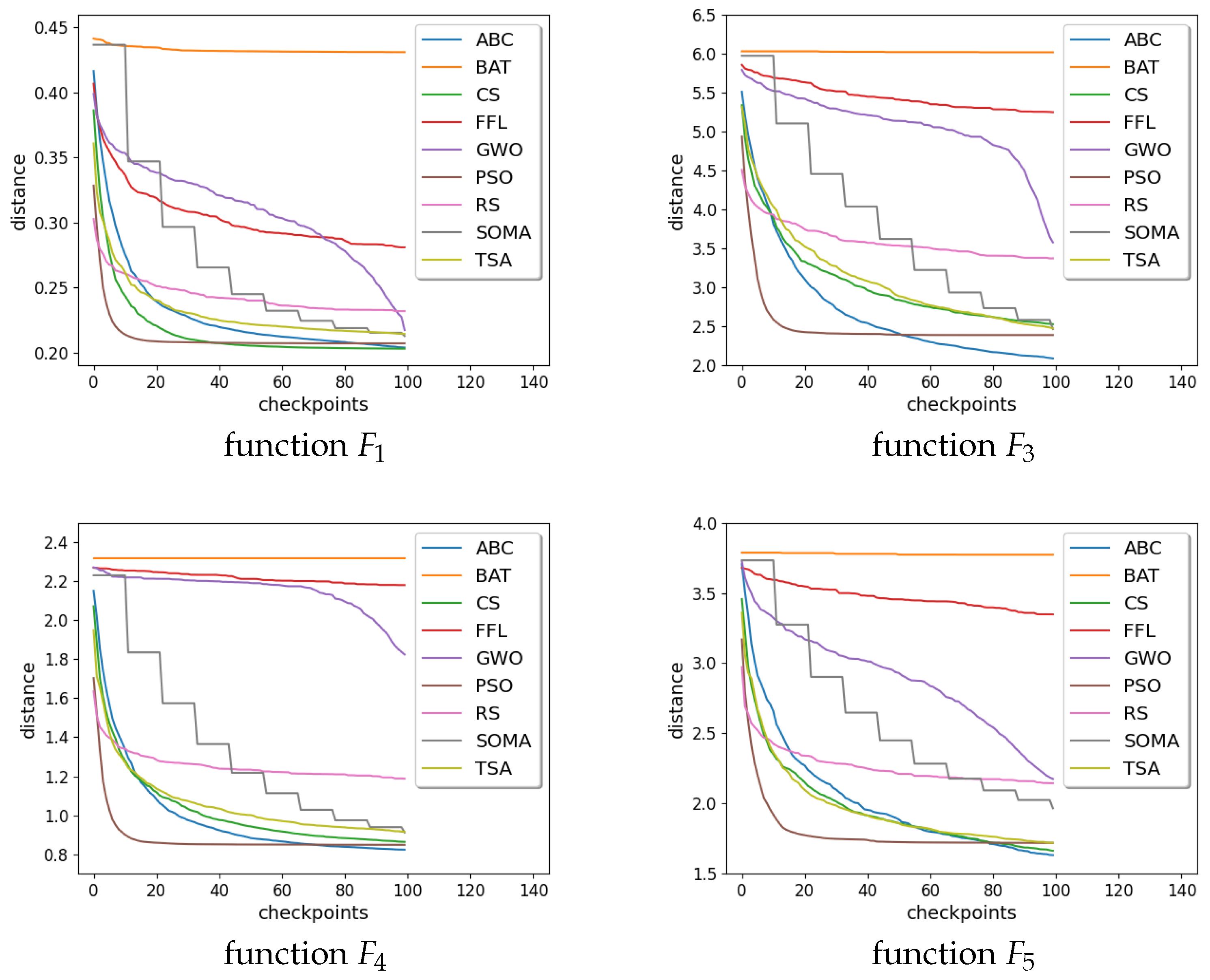
) show results of min, max, mean, median, and standard deviation values computed from 50 independent runs for each function. The following functions run with the same settings of parameters as was introduced in Section 4.2. Figure 3 and Figure 4 show graphs of distance convergence means for a selected $\mathit{maxFES}$ where checkpoints are taken each 100th iteration.

From the results (see Table 2, Table 3, Table 4 and Table 5) it is obvious that there is simply no evolutionary algorithm suitable to use for linearization of all functions. Results show that for the function $f_1$ the best algorithm is CS. On the other hand, $f_3$ and $f_4$ are best handled by the ABC algorithm. In the case of $f_5$, there is no clear which method performs the best.

If we disregard the best values for each tested function, other evolutionary algorithms can get the job done with sufficient results. We are talking mainly about PSO, SOMA, and TSA algorithms, which have results across all tested functions similar to the best results. It means that we have some degree of freedom to choose which evolutionary algorithm to use.

5. Piecewise Linearization Using Swarm Intelligence Algorithms with Automatic Parameters Tuning

In this section, we introduce an algorithm that is used for automatic detection of points ℓ used for linearization, and automatic detection of discretization points $discr\_step$ representing the length between equidistant points. This algorithm tries to find the number of input points ℓ and a set of equidistant points given by a discretization step $disc\_step$ to achieve the best possible solution evaluated based on an algorithm output fitness function value.

The main goal of this algorithm is to run a total number of six evaluations of an evolutionary algorithm in every loop iteration using parallel computing as long as it is needed to find an optimal solution. We chose to use this approach because we need to try several combinations of ℓ and $discr\_step$ in each iteration.

In the beginning, our algorithm sets the input parameters for an evolutionary algorithm and default values for $\ell =10$ and $discr\_step=1/100$. Then, the loop starts where every iteration consists of setting up six different $discr\_step$ values and six different ℓ values, and each of the six parallel runs takes one $discr\_step$ and one ℓ. The six ℓ and $discr\_step$, where ${\ell }_{i-1}$ and $discr\_ste{p}_{i-1}$ is a ℓ and $discr\_step$ of the best result from the previous iteration, can be seen in the

Table 6. Six variants of ℓ and $discr\_step$.

ℓ	$\mathit{discr}\_\mathit{step}$
${\ell }_{i-1}+3$	$discr\_ste{p}_{i-1}/1.5$
${\ell }_{i-1}+6$	$discr\_ste{p}_{i-1}/1.5$
${\ell }_{i-1}+3$	$discr\_ste{p}_{i-1}/2$
${\ell }_{i-1}+6$	$discr\_ste{p}_{i-1}/2$
${\ell }_{i-1}+3$	$discr\_ste{p}_{i-1}$
${\ell }_{i-1}$	$discr\_ste{p}_{i-1}/1.5$

.

Each of these six parallel runs is processed, and then their results are evaluated. This evaluation is done by computing the linearization provided $final\_points$ of all six results given as an output of an evolutionary algorithm run and a fixed $discr\_step=1/200$. We need to ensure that all six results are evaluated using the same evaluation criterion, which is done by setting up $discr\_step$ the same for all results. Based on this evaluation, it gives the results $final\_distance$ computed with Manhattan metric, and it keeps the result with the smallest $final\_distance$ value. The $distance$ value serves as a $fitness\_value$ for all selected evolutionary algorithms. The best results $discr\_step$, $final\_distance$, $final\_points$, and ℓ are saved to be used in the next iteration.

Next, we examine all linear segments created from $final\_points$. This examination consists of creating three equidistant points on a linear segment and calculating the distance of these points from the initial function. We always take the output of the maximum metric from all points of all linear segments. Linear segments whose slope value is too high and a maximum metric value of their equidistant points are under the set threshold are ignored. It is because they tend to get a high maximum metric output value even when these linear segments sufficiently overlap with the initial function part. The maximum of all linear segments illustrates whether the linearization is close enough to the real function or not.

At the end of every iteration, it checks whether the $fitness\_value$ value, and a maximum metric value are good enough. Thus, we check whether we should continue with the next iteration.

There is a special case when we set ${\ell }_{1,\dots ,6}={\ell }_i$ and $discr\_ste{p}_{1,\dots ,6}=discr\_ste{p}_{i-1}$ before we process parallel runs. This special case occurs when the best result from the previous iteration has a good enough $fitness\_value$ (but not a good enough maximum metric value). The idea is that the previous iteration’s best result was almost the optimal result, but the algorithm placed the final points a little off. Thus, for the next three iterations, we take all six parallel runs and use them to determine if the current $discr\_step$ and ℓ are sufficient to get an optimal solution.

It also keeps $final\_points$ of the best result and provides them to all six evolutionary algorithms run in parallel in the next iteration. This approach enables speeding-up the process of finding the optimal result by enabling an evolutionary algorithm in the next iteration to start from a position where the best result of the previous iteration ended up. The only scenario where we do not provide $final\_points$ is when the special case is triggered because we do not want to influence the parallel runs with the previous result because it was close but not close enough. Pseudocode of parameter tuning approach is in Algorithm 1.

Algorithm 1 Pseudocode of the parameter tuning algorithm.

def evaluate_evolutionary_algorithm Set evolutionary algorithm input parameters whilethe previous best results $final\_distance$ is not small enoughORthe previous results maximum metric value is not small enoughdo     set ${\ell }_{1,\dots ,6}$ and $discr\_ste{p}_{1,\dots ,6}$     if special case AND special case count <3 then         modify ${\ell }_{1,\dots ,6}$ and $discr\_ste{p}_{1,\dots ,6}$     end if     run all six parallel runs     collect all six results     compute a $final\_distance$ for all six results     select the best result of this iteration     save the best results $discr\_step$, $final\_points$, $final\_distance$, and ℓ     get a maximum metric value of the best results linear segments end while

5.1. Examples of Tuning Algorithm

In this subsection, the evolutionary algorithms selected in Section 3 will be applied to the algorithm introduced in Section 5 on Function $f_5$. Therefore, two sets of results were achieved, where the first one was achieved for $\mathit{maxFES}=2500$ and the second for $\mathit{maxFES}=$ 10,000. In both sets of results, each evolutionary algorithm optimal result should have a $final\_distance$ calculated with Manhattan distance to be equal or better than 2.0. All evolutionary algorithms use input parameter values from Section 4.2. Each experiment is executed 50 times in Python 3.8 on a computer with the CPU: AMD 2920X, RAM: 32 GB DDR4, GPU: AMD RX VEGA64. The time complexity of the compared algorithms of each run is estimated in seconds.

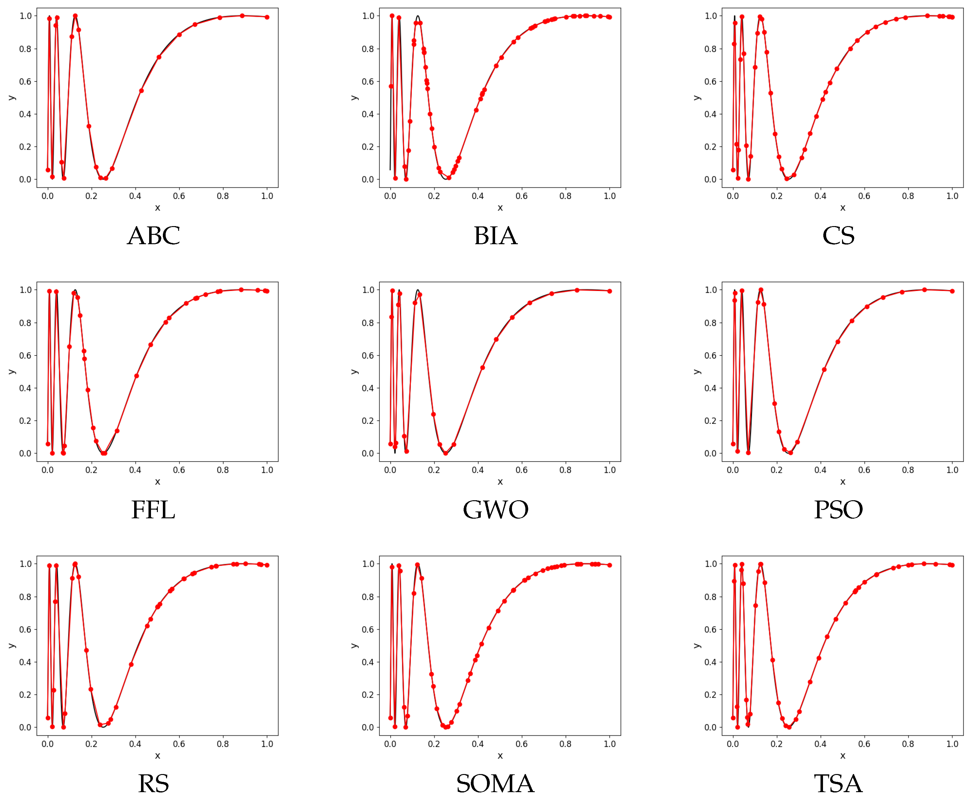
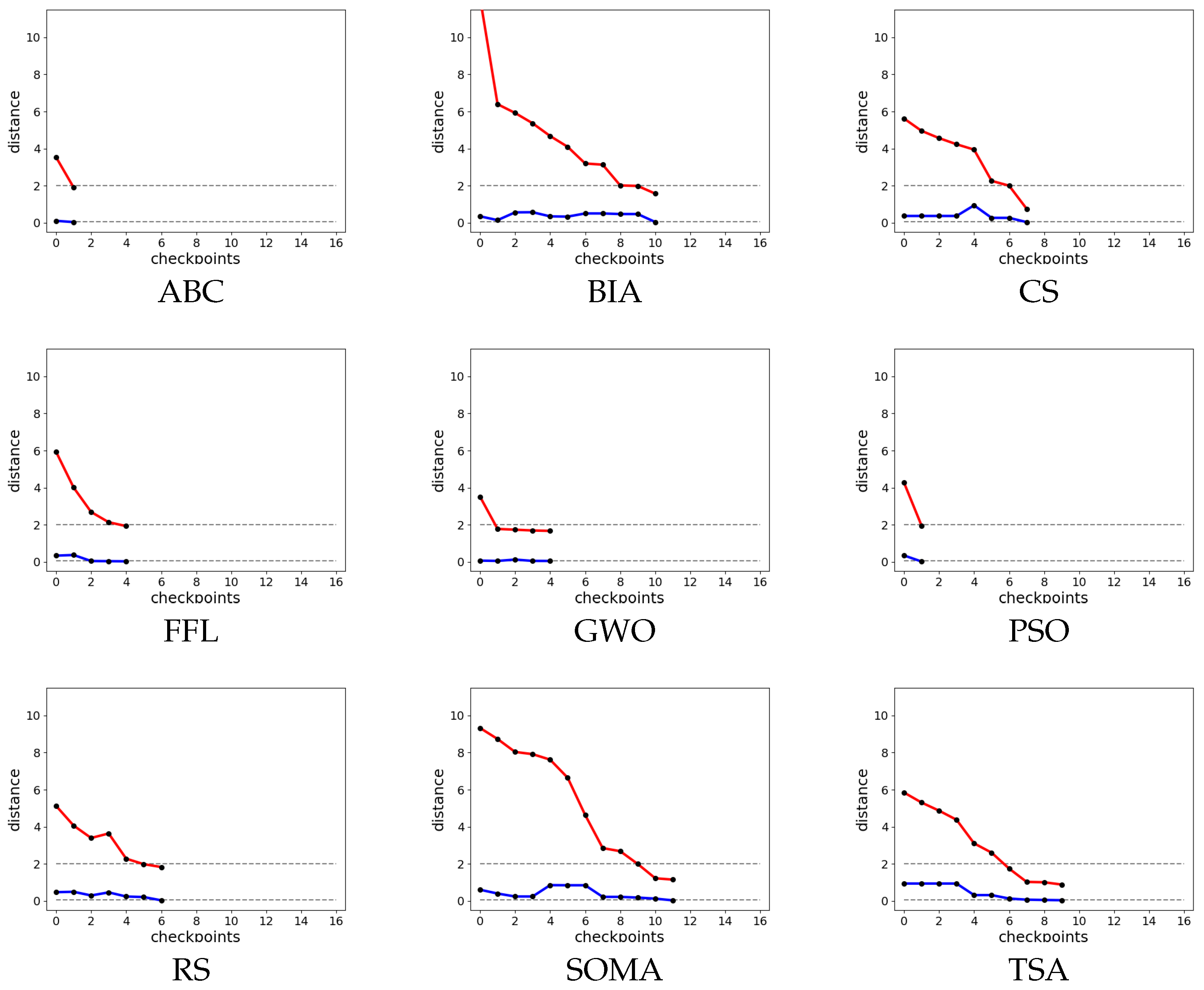
Example 1.

This example consists of the results of selected evolutionary algorithms with a value of $\mathit{maxFES}=2500$. The graph of results for Function $f_5$ approximation of each algorithm is presented (Figure 5). The best result of each parallel run is saved as a checkpoint result. Then, we take the best run out of all 50 runs and illustrate its checkpoint results in graphs in Figure 6 and

Table 7. The best results of evolutionary algorithms with a value of $\mathit{maxFES}=$ 2500.

	ℓ	Discr_Step	Final_Distance	Time (s)
PSO	22	0.003	1.945	13.16
SOMA	43	0.001	1.886	31.03
CS	52	0.001	0.845	77.26
FFL	43	0.001	1.786	22.29
GWO	22	0.004	1.961	9.74
ABC	34	0.001	1.505	30.06
BIA	61	0.001	1.670	49.82
TSA	43	0.001	1.193	31.73
RS	37	0.002	1.965	15.44

Example 2.

The second example consists of results with $\mathit{maxFES}=$ 10,000. The graph of results for Function $f_5$ approximation of each algorithm is presented (Figure 7). The best result of each parallel run is saved as a checkpoint result. Then, we take the best run out of all 50 runs and illustrate its checkpoint results in graphs in Figure 8 and

Table 8. The best results of evolutionary algorithms with a value of $\mathit{maxFES}=$ 10,000.

	ℓ	Discr_Step	Final_Distance	Time (s)
PSO	22	0.003	1.957	14.20
SOMA	49	0.001	1.149	151.99
CS	46	0.001	0.753	88.07
FFL	34	0.001	1.927	41.47
GWO	22	0.003	1.669	85.72
ABC	22	0.003	1.904	12.26
BIA	58	0.001	1.571	123.00
TSA	43	0.001	0.882	146.58
RS	37	0.001	1.827	69.51

.

5.2. Comparison Results Summary

The comparison of the algorithms mentioned in this section was done on all testing functions from Section 4.1. For demonstration, we chose only four functions, to not overwhelm readers with tables (see Functions $f_1$, $f_3$, $f_4$, and $f_5$).

We calculated the values of arithmetic mean of ℓ, $discr\_step$, $final\_distance$, and $time$ what has estimated time complexity measured in seconds from 50 runs for each testing function and each evolutionary algorithm. All 50 runs were calculated for $\mathit{maxFES}=2500$ and $\mathit{maxFES}=$ 10,000. Results show that the $\mathit{maxFES}=$ 10,000 variant offers almost the same results as $\mathit{maxFES}=2500$ variant or there is a slight decrease in a total number of points but at the expense of increasing time.

The most important value is always $final\_distance$, but we cannot decide which algorithm is the best one based only on this value. In general, we need to find the balance between $final\_distance$ and the time it takes to achieve this value where time is affected by ℓ (the higher, the worse) and $discr\_step$ (the lower, the worse). We even have to consider a situation when $final\_distance$ is good enough, but that is due to bad linearization, which results in taking longer to accomplish an optimal result. It also means that an evolutionary algorithm will need more iterations to get to this optimal result and, thus, it will have more points ℓ, which improves $final\_distance$, which takes more time. Finally, $final\_distance$ is so good thanks to the evolutionary algorithm’s inability to create a good linearization. In some cases, it is recommended to favor an evolutionary algorithm with a worse $final\_distance$ but with significantly better ℓ, $discr\_step$, and $time$.

In

Table 9. The three best evolutionary algorithms for each testing function.

Function	FES	1st	2nd	3rd
$f_1$	2500	PSO	RS	ABC
$f_3$	2500	PSO	ABC	CS
$f_4$	2500	PSO	ABC	FFL
$f_5$	2500	GWO	PSO	CS
$f_5$	10,000	PSO	ABC	GWO

, the best three algorithms for the testing functions $f_1$, $f_3$, $f_4$, and $f_5$ are presented.

Based on the finding, we decided to show only one set of results of $\mathit{maxFES}=$ 10,000 variant (see

Table 10. The mean results for Function $f_1$ for 50 runs of evolutionary algorithms with a value of $maxFES=2500$.

	ℓ	Discr_Step	Final_Distance	Time (s)
PSO	15	0.006	1.139	2.66
SOMA	15	0.005	1.413	3.21
CS	16	0.005	1.426	3.79
FFL	15	0.006	1.455	2.00
GWO	15	0.005	1.477	5.31
ABC	16	0.005	1.330	2.96
BIA	17	0.004	1.423	3.88
TSA	16	0.005	1.378	4.28
RS	15	0.006	1.283	3.01

,

Table 11. The mean results for Function $f_3$ for 50 runs of evolutionary algorithms with a value of $maxFES=2500$.

	ℓ	Discr_Step	Final_Distance	Time (s)
PSO	68	0.001	1.536	74.17
SOMA	81	0.001	1.658	119.26
CS	74	0.001	1.540	74.49
FFL	88	0.001	1.727	81.51
GWO	95	0.001	1.615	345.76
ABC	61	0.001	1.711	54.77
BIA	85	0.001	1.704	79.29
TSA	73	0.001	1.562	114.93
RS	86	0.001	1.539	114.40

,

Table 12. The mean results for Function $f_4$ for 50 runs of evolutionary algorithms with a value of $maxFES=2500$.

	ℓ	Discr_Step	Final_Distance	Time (s)
PSO	29	0.002	1.519	12.25
SOMA	34	0.001	1.682	18.02
CS	35	0.001	1.638	17.11
FFL	35	0.001	1.588	16.10
GWO	33	0.001	1.631	37.28
ABC	29	0.002	1.645	11.40
BIA	36	0.001	1.688	16.46
TSA	35	0.001	1.626	22.15
RS	35	0.001	1.666	20.64

,

Table 13. The mean results for Function $f_5$ for 50 runs of evolutionary algorithms with a value of $maxFES=2500$.

	ℓ	Discr_Step	Final_Distance	Time (s)
PSO	28	0.002	1.489	15.52
SOMA	86	0.001	1.016	142.64
CS	74	0.001	0.615	76.08
FFL	69	0.001	1.346	149.29
GWO	28	0.002	1.374	32.87
ABC	53	0.001	1.156	98.07
BIA	91	0.001	1.055	168.31
TSA	75	0.001	0.619	91.78
RS	61	0.001	1.234	108.15

and

Table 14. The mean results for Function $f_5$ for 50 runs of evolutionary algorithms with a value of $maxFES=$ 10,000.

	ℓ	Discr_Step	Final_Distance	Time (s)
PSO	27	0.002	1.463	41.41
SOMA	78	0.001	0.783	273.57
CS	73	0.001	0.422	207.79
FFL	63	0.001	1.305	331.04
GWO	25	0.002	1.495	101.53
ABC	29	0.002	1.499	53.39
BIA	94	0.001	1.021	538.83
TSA	72	0.001	0.500	280.39
RS	54	0.001	1.302	252.29

). It is obvious that the best overall evolutionary algorithm to use for linearization is PSO. Except for $f_5$ (variant $\mathit{maxFES}=2500$) where PSO ended up the second best, it was always the best evolutionary algorithm to use. Based on the results, we can also see that the ABC algorithm can also be considered as a suitable evolutionary algorithm to overall use for linearization.

5.3. Statistical Results Summary

In this section, the results of the compared algorithms will be statistically assessed. We assess whether or not our proposed method of automatic parameters tuning algorithm proves itself successful or not.

The mean ranks from the Friedman tests [31] can be seen in

Table 15. The mean ranks of all algorithms from the Friedman test.

Algorithm	PSO${}_{\mathit{s}}^{\ast }$	RS${}_{\mathit{s}}^{\ast }$	TSA${}_{\mathit{s}}^{\ast }$	ABC	RS${}^{\ast }$	SOMA${}^{\ast }$
m.rank	9.5	9.75	9.75	10	10.5	11
PSO${}^{\ast }$	PSO	ABC${}_s^{\ast }$	CS${}_s^{\ast }$	CS	ABC${}^{\ast }$	TSA${}^{\ast }$
11.5	11.5	11.75	11.75	11.75	12.375	12.75
SOMA	TSA	SOMA${}_s^{\ast }$	CS${}^{\ast }$	FFL${}_s^{\ast }$	BAT${}_s^{\ast }$	RS
13	13.5	14.25	15	15.375	15.5	15.75
GWO${}_s^{\ast }$	BAT${}^{\ast }$	GWO${}^{\ast }$	FFL${}^{\ast }$	GWO	FFL	BAT
16	16.5	16.5	19	19.75	21.5	22.5

. The results of the algorithms without tuning to the value $\mathit{maxFES}=$ 10,000 are labeled without any upper/lower index. The tuning algorithm results using $\mathit{maxFES}=$ 10,000 are labeled with an upper asterisk index. The tuning algorithm results where $\mathit{maxFES}=2500$ was set are labeled with an upper asterisk index and lower s letter index. The best three performing algorithms are variants with $\mathit{maxFES}=2500$ using a tuning algorithm. They also achieved similar results in the Friedman test, so it is a good indicator that they are all good to use for the piecewise linearization of functions.

In

Table 16. The median values for each algorithm and each set.

SET	f	ABC	BAT	CS	FFL	GWO	PSO	RS	SOMA	TSA
O10	1	0.204	0.432	0.203	0.281	0.224	0.205	0.232	0.209	0.213
O10	3	2.080	6.093	2.534	5.269	3.305	2.284	3.390	2.352	2.441
O10	4	0.820	2.230	0.855	2.207	1.808	0.828	1.184	0.882	0.914
O10	5	1.688	3.828	1.704	3.401	2.024	1.705	2.160	1.966	1.729
T10	1	1.167	1.494	1.574	1.498	1.627	1.056	1.311	1.281	1.616
T10	3	1.654	1.742	1.666	1.862	1.703	1.613	1.517	1.643	1.561
T10	4	1.630	1.721	1.736	1.764	1.518	1.647	1.636	1.685	1.702
T10	5	1.529	1.014	0.410	1.238	1.699	1.412	1.266	0.774	0.457
T25	1	1.277	1.441	1.493	1.477	1.525	1.098	1.257	1.386	1.351
T25	3	1.741	1.725	1.603	1.840	1.654	1.553	1.516	1.702	1.604
T25	4	1.601	1.718	1.686	1.627	1.689	1.545	1.664	1.710	1.644
T25	5	1.110	1.029	0.596	1.355	1.352	1.521	1.201	1.027	0.555
O25	1	0.233	0.427	0.214	0.309	0.231	0.205	0.253	0.268	0.234
O25	3	2.996	5.969	3.233	5.447	3.818	2.339	3.725	4.138	3.322
O25	4	1.024	2.387	1.056	2.246	1.962	0.819	1.297	1.381	1.083
O25	5	2.129	3.726	2.025	3.457	2.652	1.785	2.399	2.480	1.987

are the median values for each algorithm and each setting. There are four different settings: O10 and O25 are the original algorithms with $\mathit{maxFES}=2500$ (O25) and 10,000 (O10). The T10 and T25 settings represent the automatic-parameter-tuning versions with $maxFES=2500$ (T25) and 10000 (T10). For O10, the best algorithm is ABC. On the other hand, O25 is the best to use with PSO. Results of setting variants T10 and T25 are not that straightforward, but it is obvious that the PSO algorithm is the overall best choice to use.

The next level of statistical comparison provides the Kruskal–Wallis test [32] (see

Table 17. The first, second, third, and the last position of all algorithms and each setting from the Kruskal–Wallis tests.

SET	f	Sig.	1st	2nd	3rd	Last
O10	1	<0.001	CS	ABC	PSO	BAT
O10	3	<0.001	ABC	PSO	SOMA	BAT
O10	4	<0.001	ABC	PSO	CS	BAT
O10	5	<0.001	ABC	CS	TSA	BAT
T10	1	<0.001	PSO	ABC	SOMA	TSA
T10	3	<0.001	RS	TSA	PSO	FFL
T10	4	<0.01	GWO	ABC	PSO	CS
T10	5	<0.001	CS	TSA	SOMA	ABC
T25	1	<0.001	PSO	RS	ABC	GWO
T25	3	<0.001	RS	PSO	CS	FFL
T25	4	<0.05	PSO	FFL	GWO	BAT
T25	5	<0.001	CS	TSA	SOMA	PSO
O25	1	<0.001	PSO	CS	ABC	BAT
O25	3	<0.001	PSO	ABC	CS	BAT
O25	4	<0.001	PSO	ABC	CS	BAT
O25	5	<0.001	PSO	TSA	CS	BAT

). This method provides us with the same results as Table 16. The variant O10 is the best to use together with the ABC algorithm. The variant O25, on the other hand, is the best to use together with the PSO algorithm. We cannot say which algorithm to use together with T10 and T25 variants because there is no straightforward choice suitable for all tested functions. Overall, the best choice would be the PSO algorithm which can be found in the first place most times compared to the rest of the algorithms.

Finally, the results of the Wilcoxon rank-sum statistical test [33] are presented (see

Table 18. The median values and significance of all algorithms from the Wilcoxon rank-sum tests.

f	alg	T25	T10	O10
1	ABC	1.2768	1.1673($++$)	0.20377($+++$)
1	BAT	1.4415	1.4942(≈)	0.43178($+++$)
1	CS	1.4928	1.574(−)	0.20281($+++$)
1	FFL	1.4774	1.4976(≈)	0.28131($+++$)
1	GWO	1.5246	1.627(≈)	0.22386($+++$)
1	PSO	1.098	1.0557(≈)	0.20484($+++$)
1	RS	1.2572	1.3113(≈)	0.23168($+++$)
1	SOMA	1.3856	1.2814(≈)	0.20902($+++$)
1	TSA	1.3507	1.6165($---$)	0.21299($+++$)
3	ABC	1.7409	1.654(≈)	2.0797($---$)
3	BAT	1.7248	1.7422(≈)	6.0932($---$)
3	CS	1.603	1.6659(≈)	2.5338($---$)
3	FFL	1.8396	1.8621(≈)	5.2694($---$)
3	GWO	1.6536	1.7029(≈)	3.3049($---$)
3	PSO	1.5535	1.6128(≈)	2.2837($---$)
3	RS	1.5156	1.5173(≈)	3.3899($---$)
3	SOMA	1.7017	1.6433(≈)	2.3522($---$)
3	TSA	1.6039	1.5613(≈)	2.4407($---$)
4	ABC	1.6015	1.6296(≈)	0.82008($+++$)
4	BAT	1.7178	1.7211(≈)	2.2302($---$)
4	CS	1.6855	1.7358(≈)	0.85474($+++$)
4	FFL	1.6296	1.7641(−)	2.2069($---$)
4	GWO	1.6887	1.5177(+)	1.808($---$)
4	PSO	1.5454	1.6473(−)	0.82815($+++$)
4	RS	1.6641	1.6358(≈)	1.1841($+++$)
4	SOMA	1.7101	1.6848(≈)	0.88182($+++$)
4	TSA	1.6438	1.7023(≈)	0.91401($+++$)
5	ABC	1.1098	1.5286($---$)	1.6882($---$)
5	BAT	1.0294	1.0142(≈)	3.8278($---$)
5	CS	0.5961	0.4104($+++$)	1.7042($---$)
5	FFL	1.3547	1.2379(≈)	3.4007($---$)
5	GWO	1.3519	1.6986(≈)	2.0238($---$)
5	PSO	1.5213	1.4122(≈)	1.7051($---$)
5	RS	1.2013	1.2659(≈)	2.1597($---$)
5	SOMA	1.0273	0.77375($+++$)	1.9665($---$)
5	TSA	0.5553	0.45704($++$)	1.7291($---$)

). The variant T25 was selected as a reference method, and it is compared against variants T10 and O10. The symbol of ‘+’ is used for significantly better results of counterpart, a symbol of ‘−’ is used for significantly better results of reference method, and finally, the symbol of ‘≈’ illustrates no significant difference between algorithms. The comparison of T25 and T10 shows only several significant differences between settings, so it is obvious that these two variants score very similarly. Both variants seem to find good results very quickly, and thanks to this, the importance of $\mathit{maxFES}$ is not that high. Comparing T25 and O10, there are 15 cases where the O10 variant performs significantly better than the T25 variant (especially for problem $f_1$), but there are 21 cases in total when the O10 variant is significantly worse than the variant T25. We can interpret the results slightly different, though. The variant T25 delivers more consistent results across all cases, whereas the O10 variant delivers either very good or very bad results.

Results also show that the non-tuning algorithm suffers from lowering $\mathit{maxFES}$ from 10,000 to 2500, and that is the reason we did not include the O10 variant at all. On the other hand, the automatic parameters tuning algorithm is resistant to the length of the optimization process, therefore, it does not matter if we choose the value of $\mathit{maxFES}=$ 2500 or 10,000.

6. Conclusions

In this paper, we introduced two ways to solve the optimization of the piecewise linearization of a given function. In the first approach, the usage of optimization algorithms for searching piecewise linearization with a predefined number of piecewise linear parts and discretization points with the calculation of the distance between the original and piecewise linear function is proposed. The second method extends the previous approach by the automatic selection of the number of piecewise linear parts and discretization points.

Based on the experimental part of the paper, the following conclusions were achieved. Enhancing the swarm-based optimization algorithms by the proposed tuning approach enables a significant increase in the performance of the optimization process. When the algorithms were applied to the piecewise linearization problem with 2500 function evaluations, the variants of PSO and GWO provided sufficient results, where GWO performs substantially better (Table 7). For $\mathit{maxFES}=$ 10,000, GWO, PSO, and ABC provide results with a similar quality, where ABC was the fastest method (Table 8).

From the results of the optimization problems, it is obvious that the variant of PSO was always located on the best positions (Table 10, Table 11, Table 12, Table 13 and Table 14, ). Moreover, a variant of ABC provided an acceptable quality solution (Table 9). Studying the complexity of the compared algorithms, the variants of PSO and ABC achieved mostly low time demands.

Results of the application of the proposed tuning approach illustrate the substantially increasing performance of the compared swarm algorithms (Table 15). In eight algorithms out of nine, the better overall performance was achieved by the tuning approach, where the biggest difference was achieved in variant of RS, which provided second-best results. It is also obvious that several swarm methods provide worse results compared to the simple RS method, which generates random solutions (BAT, FFL, GWO).

Comparing the achieved median values in three out of four optimization problems, the best performance is provided with the proposed tuning approach (Table 16). Surprisingly, the best results of the piecewise linearization problem $f_4$ provided the RS algorithm with the tuning mechanism.

The main benefit of our tuning approach is the lower time complexity of the optimization process (measured by a number of function evaluations) with sufficient solutions. Using the PSO algorithm as the main swarm intelligence algorithm for solving piecewise linearization problems is, without a doubt, the best choice. This conclusion was clearly demonstrated in Section 5.3.

The proposed tuning approach performs worse than the original swarm intelligence algorithms, especially in problem $f_1$. This provides motivation to further study the approach settings. The first step in the research is to generalize the proposed algorithms for functions with higher dimensions and use them for solving other real problems.

The next natural step is to extend this algorithm into higher dimensions and to compare the swarm-based optimization algorithms with the classical mathematical approaches.

References

- Kontogiorgis, S. Practical piecewise-linear approximation for monotropic optimization. INFORMS J. Comput. 2000, 12, 324–340. [Google Scholar] [CrossRef]
- Kupka, J.; Škorupová, N. On PSO-Based Simulations of Fuzzy Dynamical Systems Induced by One-Dimensional Ones. Mathematics 2021, 9, 2737. [Google Scholar] [CrossRef]
- Kupka, J.; Škorupová, N. On PSO-Based Approximation of Zadeh’s Extension Principle. In Proceedings of the International Conference on Information Processing and Management of Uncertainty in Knowledge-Based Systems, Lisbon, Portugal, 15–19 June 2020; pp. 267–280. [Google Scholar]
- Bagwell, S.; Ledger, P.D.; Gil, A.J.; Mallett, M.; Kruip, M. A linearised hp–finite element framework for acousto-magneto-mechanical coupling in axisymmetric MRI scanners. Int. J. Numer. Methods Eng. 2017, 112, 1323–1352. [Google Scholar] [CrossRef]
- Lifton, J.; Liu, T. Ring artefact reduction via multi-point piecewise linear flat field correction for X-ray computed tomography. Opt. Express 2019, 27, 3217–3228. [Google Scholar] [CrossRef] [PubMed]
- Griewank, A. On stable piecewise linearization and generalized algorithmic differentiation. Optim. Methods Softw. 2013, 28, 1139–1178. [Google Scholar] [CrossRef]
- Persson, J.; Söder, L. Comparison of threes linearization methods. In Proceedings of the PSCC2008, 16th Power System Computation Conference, Glasgow, Scotland, 14–18 July 2008. [Google Scholar]
- Dyke, P. An Introduction to Laplace Transforms and Fourier Series; Springer: London, UK, 2014. [Google Scholar]
- Perfilieva, I. Fuzzy transforms: Theory and applications. Fuzzy Sets Syst. 2006, 157, 993–1023. [Google Scholar] [CrossRef]
- Bernard, P.; Wu, L. Stochastic linearization: The theory. J. Appl. Probab. 1998, 35, 718–730. [Google Scholar] [CrossRef]
- Hatanaka, T.; Uosaki, K.; Koga, M. Evolutionary computation approach to Wiener model identification. In Proceedings of the 2002 Congress on Evolutionary Computation. CEC’02 (Cat. No. 02TH8600), Honolulu, HI, USA, 12–17 May 2002; Volume 1, pp. 914–919. [Google Scholar]
- Mazarei, M.M.; Behroozpoor, A.A.; Kamyad, A.V. The Best Piecewise Linearization of Nonlinear Functions. Appl. Math. 2014, 5, 3270. [Google Scholar] [CrossRef]
- Cleghorn, C.W.; Engelbrecht, A.P. Piecewise linear approximation of n-dimensional parametric curves using particle swarms. In Proceedings of the International Conference on Swarm Intelligence, Brussels, Belgium, 12–14 September 2012; Springer: Berlin/Heidelberg, Germany, 2012; pp. 292–299. [Google Scholar]
- Ghosh, S.; Ray, A.; Yadav, D.; Karan, B. A genetic algorithm based clustering approach for piecewise linearization of nonlinear functions. In Proceedings of the 2011 International Conference on Devices and Communications (ICDeCom), Mesra, India, 24–25 February 2011; pp. 1–4. [Google Scholar]
- Liu, L.; Fan, Z.; Wang, X. A Piecewise Linearization Method of Significant Wave Height Based on Particle Swarm Optimization. In Proceedings of the International Conference in Swarm Intelligence, Harbin, China, 12–15 June 2013; Springer: Berlin/Heidelberg, Germany, 2013; pp. 144–151. [Google Scholar]
- Topaloglu, H.; Powell, W.B. An algorithm for approximating piecewise linear concave functions from sample gradients. Oper. Res. Lett. 2003, 31, 66–76. [Google Scholar] [CrossRef]
- Camponogara, E.; Nazari, L.F. Models and algorithms for optimal piecewise-linear function approximation. Math. Probl. Eng. 2015, 2015, 876862. [Google Scholar] [CrossRef]
- Bujok, P.; Tvrdik, J.; Polakova, R. Nature-Inspired Algorithms in Real-World Optimization Problems. MENDEL 2017, 23, 7–14. [Google Scholar] [CrossRef][Green Version]
- Bujok, P.; Tvrdik, J.; Polakova, R. Comparison of nature-inspired population-based algorithms on continuous optimisation problems. Swarm Evol. Comput. 2019, 50, 100490. [Google Scholar] [CrossRef]
- Poli, R.; Kennedy, J.; Blackwell, T. Particle swarm optimization. Swarm Intell. 2007, 1, 33–57. [Google Scholar] [CrossRef]
- Eberhart, R.; Kennedy, J. Particle swarm optimization. In Proceedings of the IEEE International Conference on Neural Networks, Perth, WA, Australia, 27 November–1 December 1995; Citeseer: Perth, WA, Australia, 1995; Volume 4, pp. 1942–1948. [Google Scholar]
- Kennedy, J. Particle swarm optimization. Encycl. Mach. Learn. 2010, 760–766. [Google Scholar] [CrossRef]
- Zelinka, I. SOMA-Self-Organizing Migrating Algorithm. In New Optimization Techniques in Engineering; Springer: Berlin/Heidelberg, Germany, 2004; pp. 167–217. [Google Scholar]
- Yang, X.S.; Deb, S. Cuckoo search via Lévy flights. In Proceedings of the 2009 World Congress on Nature & Biologically Inspired Computing (NaBIC), Coimbatore, India, 9–11 December 2009; pp. 210–214. [Google Scholar]
- Yang, X.S. Firefly algorithm, Levy flights and global optimization. In Research and Development in Intelligent Systems XXVI; Springer: Berlin/Heidelberg, Germany, 2010; pp. 209–218. [Google Scholar]
- Mirjalili, S.; Mirjalili, S.M.; Lewis, A. Grey wolf optimizer. Adv. Eng. Softw. 2014, 69, 46–61. [Google Scholar] [CrossRef]
- Karaboga, D.; Basturk, B. Artificial bee colony (ABC) optimization algorithm for solving constrained optimization problems. In Proceedings of the International Fuzzy Systems Association World Congress, Cancun, Mexico, 18–21 June 2007; Springer: Berlin/Heidelberg, Germany, 2007; pp. 789–798. [Google Scholar]
- Yang, X.S. A new metaheuristic bat-inspired algorithm. In Nature Inspired Cooperative Strategies for Optimization (NICSO 2010); Springer: Berlin/Heidelberg, Germany, 2010; pp. 65–74. [Google Scholar]
- Kiran, M.S. TSA: Tree-seed algorithm for continuous optimization. Expert Syst. Appl. 2015, 42, 6686–6698. [Google Scholar] [CrossRef]
- Rastrigin, L. The convergence of the random search method in the extremal control of a many parameter system. Autom. Remote Control 1963, 24, 1337–1342. [Google Scholar]
- Friedman, M. A Comparison of Alternative Tests of Significance for the Problem of m Rankings. Ann. Math. Stat. 1940, 11, 86–92. [Google Scholar] [CrossRef]
- Kruskal, W.H.; Wallis, W.A. Use of Ranks in One-Criterion Variance Analysis. J. Am. Stat. Assoc. 1952, 47, 583–621. [Google Scholar] [CrossRef]
- Wilcoxon, F. Individual Comparisons by Ranking Methods. Biom. Bull. 1945, 1, 80–83. [Google Scholar] [CrossRef]
Figure 1.
Graphs of the functions , , , , , and .
Figure 2.
Each graph represents the best result of a specific algorithm. The total number of points was set to 16 and 10,000.
Figure 3.
Graphs of distance convergence means for .
Figure 4.
Graphs of distance convergence means for 10,000.
Figure 5.
Graphs of algorithms with a value of .
Figure 6.
Checkpoints of each algorithm automatic parameter tuning with 2500. Red lines
are values of final_distance and blue ones show the maximum value of Manhattan distance. Grey
dashed lines show values thresholds.
Figure 7.
Graphs of algorithms with a value of 10,000.
Figure 8.
Checkpoints of each algorithm automatic parameter tuning with 10,000. Red lines are values of and blue ones show the maximum value of Manhattan distance. Grey dashed lines show values thresholds.