All articles published by MDPI are made immediately available worldwide under an open access license. No special
permission is required to reuse all or part of the article published by MDPI, including figures and tables. For
articles published under an open access Creative Common CC BY license, any part of the article may be reused without
permission provided that the original article is clearly cited. For more information, please refer to
https://www.mdpi.com/openaccess.
Feature papers represent the most advanced research with significant potential for high impact in the field. A Feature
Paper should be a substantial original Article that involves several techniques or approaches, provides an outlook for
future research directions and describes possible research applications.
Feature papers are submitted upon individual invitation or recommendation by the scientific editors and must receive
positive feedback from the reviewers.
Editor’s Choice articles are based on recommendations by the scientific editors of MDPI journals from around the world.
Editors select a small number of articles recently published in the journal that they believe will be particularly
interesting to readers, or important in the respective research area. The aim is to provide a snapshot of some of the
most exciting work published in the various research areas of the journal.
Partial differential equation (PDE) based surfaces own a lot of advantages, compared to other types of 3D representation. For instance, fewer variables are required to represent the same 3D shape; the position, tangent, and even curvature continuity between PDE surface patches can be naturally maintained when certain conditions are satisfied, and the physics-based nature is also kept. Although some works applied implicit PDEs to 3D surface reconstruction from images, there is little work on exploiting the explicit solutions of PDE to this topic, which is more efficient and accurate. In this paper, we propose a new method to apply the explicit solutions of a fourth-order partial differential equation to surface reconstruction from multi-view images. The method includes two stages: point clouds data are extracted from multi-view images in the first stage, which is followed by PDE-based surface reconstruction from the obtained point clouds data. Our computational experiments show that the reconstructed PDE surfaces exhibit good quality and can recover the ground truth with high accuracy. A comparison between various solutions with different complexity to the fourth-order PDE is also made to demonstrate the power and flexibility of our proposed explicit PDE for surface reconstruction from images.
Surface reconstruction from images is the process of recovering the 3D geometry and structure of objects and scenes based on the information of one or multiple images. It is a widely and deeply researched topic that has been commonly adopted in many areas, such as medical diagnosis, quality inspection, cultural heritage and scene understanding [1,2,3]. Generally, there are two types of methods to achieve this task. Methods of the first type decompose the reconstruction process into two steps; in the first step, 3D point clouds or volumetric data are extracted from multiple images or a single image, followed by 3D surface reconstruction from the 3D point cloud or volumetric data obtained from the previous step [4,5,6]. Methods of the second type just reconstruct a 3D surface from multiple images or a single image without generating intermediate datasets [7,8,9].
Regarding the types of representation of reconstructed surfaces, they mainly can be divided into two classes: explicit surfaces (such as B-spline and NURBS surfaces) and implicit surfaces (such as level set). Both have been widely adopted in surface reconstruction from 2D images, as discussed in Section 2. However, all these methods have some drawbacks in common; specifically, they require big data storage and heavy geometry processing.
To overcome the limitations of the existing representation of the 3D surface, we propose to reconstruct a PDE-based 3D surface from multiple-view 2D images by applying the explicit solutions of a fourth-order PDE. Compared to other types of 3D representation, PDE-based surfaces have many advantages. First of all, less data storage is required to represent the same 3D shape. Furthermore, the position, tangent and even curvature continuity between adjacent PDE patches can be naturally maintained when certain boundary conditions are met. Thirdly, parameters and sculpting forces in PDE can be adjusted and applied respectively to make the PDE model more powerful and flexible, which can also be achieved by combining the explicit solutions of PDE.
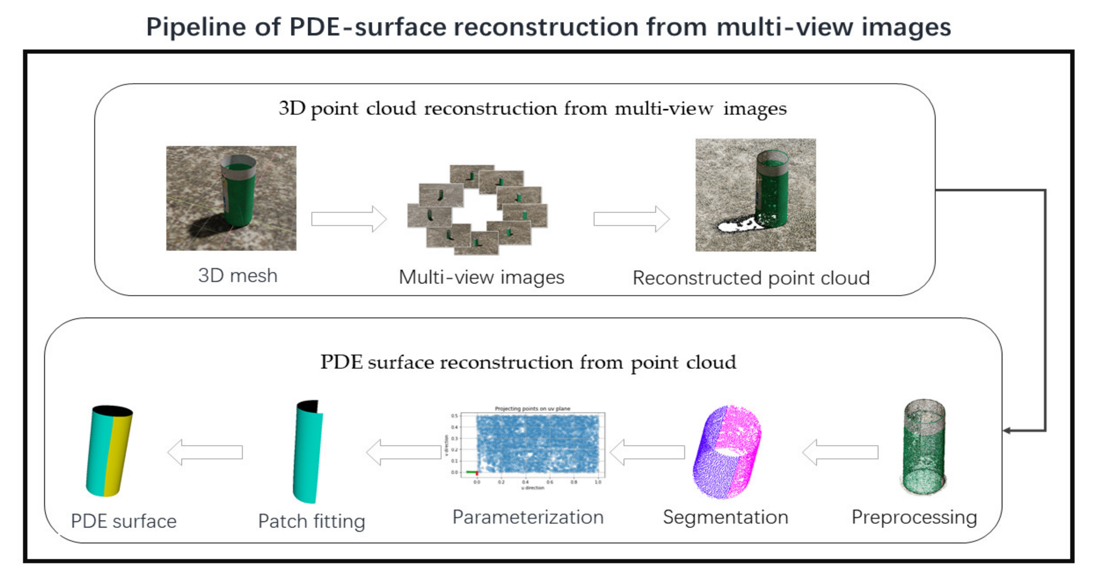
In this paper, we follow the scheme of the first type of method to reconstruct a 3D PDE-based surface from multi-view images, as it is more suitable for our proposed model. Figure 1 shows the general pipeline of our proposed method for PDE surface reconstruction PDE from multiple images. It proceeds as follows: firstly, 3D point clouds data will be reconstructed from multiple-view images; then, the PDE-based surface is obtained by fitting it to the reconstructed point clouds data. To be more concrete, in the first step, many algorithms reported in the literature can be applied to reconstruct 3D point clouds from multiple 2D images of certain objects or scenes, and they have various characteristics, so choosing a suitable algorithm for a certain object is necessary. Since multiple images of certain objects or scenes are required to reconstruct 3D point clouds data, we also have to consider how to obtain such multiple images. In this paper, we consider synthetic multi-view 2D images data of a chosen 3D object as rendered from multiple views by using the popular open-source 3D computer graphics software, Blender. When it comes to the next step, reconstructing the PDE surface from point clouds data also consists of several sub-steps, including filtering obtained point clouds data from the last step, segmenting the point clouds into multiple subsets when necessary, parameterizing the point clouds in each subset, and fitting the PDE patch to each parameterized point clouds subset; finally, the PDE surface is reconstructed. Details about all these procedures are given in Section 3.
Following the pipeline of surface reconstruction from multi-view images, the remaining sections of this paper are structured as follows: In Section 2, related work about 3D reconstruction, including 3D point clouds and 3D surfaces, from multiple images or a single image is introduced. The proposed PDE model and its analytical solutions are given in Section 3. We then focus on the proposed method of 3D point clouds reconstruction from multi-view images and PDE-based 3D surface reconstruction from obtained point clouds data in Section 4. In Section 5, the empirical results and some analysis are shown, including effects comparison between various combinations of explicit solutions to a fourth-order PDE on the reconstructed result. Finally, we conclude this paper and give some ideas about future work in Section 6.
2. Related Work
Several methods have been proposed for 3D surface reconstruction from images. They can mainly be divided chronologically into two periods [10]. In the first period, researchers tried to solve this problem from the perspective of geometry; specifically, they tried to find the projecting relationship between 3D objects and their corresponding 2D images taken from different angles, targeting at devising mathematical solutions to the ill-posed inverse problem. Generally, such methods require multiple images covering the whole object to be reconstructed. For example, a technique named structure from motion (SfM) [11,12,13,14] takes images collections as input, and 3D sparse point clouds of targeted 3D objects or scene is reconstructed. Dense point clouds from multiple images can be reconstructed using a technique named multi-view stereo (MVS); related research about MVS can be found in [15,16,17,18]. Then, the obtained 3D point clouds from this step are used to reconstruct the 3D surface. For example, Wang [19] proposed a method to reconstruct curve networks from unorganized spatial points, which can be used to reconstruct 3D surfaces. A survey of 3D surface reconstruction from images can be found in [20]. A major drawback of these early methods is that they require multiple images of the same 3D object or scene from various viewpoints, which can be impractical in some scenarios.
To overcome these drawbacks, neural networks have been applied to 3D surface reconstruction from a fewer number of 2D images or even just one image. Especially with the availability of large data set, neural networks have been adopted to 3D surface reconstruction in recent years and achieved promising results. From the perspective of the chosen representation type of the output, there are mainly three types of representation that have been adopted by neural networks: volumetric representation, surface-based representation and intermediation. For example, Lei et al. [21] designed a novel neural network capable of reconstructing 3D surfaces with high quality from one or more views and preserving accurate 2D–3D correspondences. Kato et al. [22] proposed a method to reconstruct a 3D shape from a single image by innovatively integrating mesh rendering into neural networks; the reconstructed mesh can be obtained by applying learned deformation to a generic template. Refs. [23,24] decomposed the task of 3D reconstruction from images into sequential steps, and the modules in each step are trained together; the intermediate representation is normally 2.5 depth maps. Concretely, Sun et al. [23] designed a novel model that can reconstruct a 3D shape and estimate pose simultaneously; its 2.5D sketches were first predicted, followed by regressing the 3D shape. The performance of the model can be improved by integrating multi-task learning. Another study also applied neural networks to 3D point clouds reconstruction from image collections or a single image, followed by 3D surface reconstruction from point clouds. Fu et al. [25] conducted a literature review about applying deep learning in 3D reconstruction from a single image. Mandikal et al. [26] proposed a latent embedding matching approach for point clouds reconstruction from a single image. The ill-posed problem of 3D reconstruction from a single image is addressed by their proposed two-pronged method. Other methods about 3D point clouds reconstruction from a single image can also be found in [27,28,29,30].
Apart from the aforementioned methods, some other methods directly applied various 3D surface representation-based methods to 3D reconstruction from images without applying neural networks. For example, Saini [7] proposed a geometric inverse algorithm to reconstruct NURBS curves and surfaces from their arbitrary perspective images, which was achieved by fitting NURBS to the digital data in the input images. Zhao and Mohr [8,9] proposed methods to reconstruct B-spline surface patches from image sequences. Some works also applied PDE to 3D surface reconstruction from 2D images. Zaheer et al. [31] used lines and planes to reconstruct multi-planar buildings and man-made structures from a single image. Zou [32] proposed a PDE model that took 2D parallel slices as input and reconstruct 3D smooth surfaces, but this method assumed that the surfaces to be reconstructed are defined by the zero isosurfaces of the volumes. Duan et al. [33] used PDE-based deformable surfaces to evolve to fit the boundary and the topological structure of the data, which can be volumetric data, 3D point clouds and 2D images; when multiple views are available, their model can select the best view for reconstruction automatically. Please refer to [34] for an overview of surface reconstruction using PDE.
As discussed above, the application of explicit solutions of PDEs to surface reconstruction from images has been scarcely addressed in the literature. Aimed at filling this gap, in this paper, we propose a new method that uses explicit solutions of a fourth-order PDE to solve the surface reconstruction problem from multi-view images.
3. PDE Model
In our previous work [35], we proposed a fourth-order partial differential equation, obtained its closed form solutions, and used one of the obtained closed form solutions to test the applicability of the proposed method in surface reconstruction by reconstructing several simple surface patches from several sets of a few ordered points uniformly sampled from a known surface. In this paper, we extend the closed form solutions obtained in [35] from 16 vector-valued variables to 64 vector-valued variables to greatly raise the capacity in surface reconstruction and improve reconstruction quality, propose a pipeline of surface reconstruction from multi-view 2D images, and make a comparison between the method proposed in this paper and a polygon-based surface reconstruction method to demonstrate the effectiveness and advantages of the proposed method.
According to [35], the partial differential equation used for surface reconstruction can be a fourth-order partial differential equation given in Equation (1) below. The solution to the partial differential equation represents a parametric surface. In the equation, the parametric variables and are typically defined on the unit interval [0, 1], forming the four boundaries of the PDE-based surface patch.
where , , , and are vectors of the , and coordinates. can be treated as a sculpting force to make our proposed PDE model more powerful regarding reconstructing 3D surfaces; setting it to be zero, Equation (1) can be treated as a homogenous partial differential equation. To solve it analytically, we suppose that the parametric variables of the solution of Equation (1) can be linearly separated. Then, applying the separation of variables method, the solution can be written as
Inserting Equation (2) into Equation (1) and solving it analytically under different conditions, we obtain four closed-form solutions. More detailed solving procedures can be referenced in our previous work [35]. We choose one of the solutions as the PDE model to reconstruct the PDE-based surface from multi-view 2D images, shown in Equation (3).
where
where are the vector-valued unknowns.
There are 16 vector-valued unknowns in Equation (3), which can be used to reconstruct a single surface patch. However, complex shapes can rarely be represented accurately through a single patch. Generally, multiple patches are required for complicated shapes, each defined by Equation (3). Unfortunately, this solution may not be adequate in some instances. For example, it is not easy to segment complicated 3D point clouds into an appropriate number of subsets automatically. This problem can be addressed by enlarging the number of unknown variables in Equation (3), thus providing extra degrees of freedom to the problem. To achieve this, we can obtain more complex and powerful solutions by combining the solutions to the fourth-order partial differential equation under different conditions. Then, can be updated to as follows:
Conducting the multiplication operations in Equation (5) and letting
then Equation (5) can be expressed as follows:
We demonstrate how to fit our PDE models and to the reconstructed 3D point clouds data from multiple images in Section 4, which also means to find 16 unknown vector-valued variables in and 64 unknown vector-valued variables in .
4. PDE-Based Surface Reconstruction from Multi-View Images
As discussed in Section 1, the proposed method consists of the following steps: 1, generation of the multi-view images from the 3D object or scene; 2, point clouds reconstruction from the multi-view images; and 3, PDE-based 3D surface reconstruction from the obtained point clouds data.
4.1. Multi-View Images Generation
The first step consists of obtaining a collection of suitable multi-view images from a given 3D object or scene. This task is more challenging than it seems at first sight, as it requires the images to cover the entire surface of the object for a proper reconstruction. The multi-view images can be obtained either manually or automatically; the former method means we take multi-view images of a certain object with a professional camera or just our smartphone, which is not easy and is inconvenient; we can also obtain multi-view images of a certain object automatically by taking advantage of the rendering function of the software. For example, Bianco et al. “created a plug-in module for the Blender software to support the creation of synthetic datasets” [36], aiming to evaluate the performance of the structure from motion pipelines. In this paper, the multi-view images are obtained automatically using Blender software. However, there are also many factors that should be taken into consideration before starting rendering multi-view images of an object. First of all, the object to be reconstructed should own a varied texture; the number of rendering images must cover the entire surface of the object, and the rendering images should be of high quality to ensure better 3D point clouds data. We should set up the scene and render details carefully to meet these requirements. Figure 2 shows the set-up scene and the rendered multi-view 2D images by rotating the camera around the object every five degrees, so 36 rendered images cover the whole object; only 9 of the 36 images are shown in Figure 2b for clarity. These rendered images are used as the input of specialized algorithms for point clouds reconstruction from multi-view images, as explained in the next section.
4.2. Point Cloud Reconstruction from Multi-View Images
As discussed in Section 2, there are many algorithms suitable for point clouds reconstruction from multi-view images. In this paper, we consider three of them: Colmap, VisualSFM [37] and Meshroom. Multi-view 2D images are fed into each algorithm, leading to different 3D point clouds. Then, we compare the outputs to select the one that is most complete among the three methods.
Figure 3b shows the reconstructed result obtained from the Meshroom algorithm. As shown in Figure 3b, the point cloud reconstructed with the Meshroom algorithm is incomplete. When using the VisualSFM algorithm, the reconstructed point cloud is similar to the one obtained from the Meshroom algorithm. Therefore, both Meshroom and VisualSFM algorithms are not suitable. In contrast, the point cloud reconstructed with the Colmap algorithm is complete as shown in Figure 3c.
As discussed above, the Colmap algorithm provides the best results among the three algorithms. Therefore, this paper selects it to reconstruct point clouds from images. Figure 4 shows the process of 3D point cloud reconstruction from multi-view 2D images using the Colmap algorithm.
4.3. PDE-Based Surface Reconstruction from Point Clouds
4.3.1. Segmentation and Parameterization of Point Cloud
When the 3D shape defined by the point cloud is complicated, it is necessary to segment the point cloud into several smaller subsets; each subset is fitted through a PDE-based surface patch, and the final PDE surface is obtained by combining those patches.
Some point cloud segmentation methods have been proposed. According to [38], they can be divided into edge-based methods, region-growing methods, model-fitting methods, hybrid methods, and machine-learning-based methods. Edge-based methods consist of edge detection to divide a point cloud into different regions and grouping points inside each of the regions to obtain segmented subsets. Region-growing methods grow one or more seed points into a region with similar characteristics, such as surface orientation and curvature. Model-fitting methods fit a primitive, such as planes, cylinders and spheres, onto point cloud data and label the points conforming to the mathematical representation of the primitive as one segment. Hybrid methods combine more than one segmentation method to achieve the segmentation of point clouds. In recent years, machine-learning-based segmentation has attracted growing interest. A comprehensive survey on segmentation of point clouds with deep learning was made in [39].
Although various segmentation methods have been proposed, it is still a good approach to use different segmentation methods to target the segmentation of different point clouds. For the point clouds used in this paper, the point clouds for the cylinder, hat and car models will be segmented into subsets for reconstructing their PDE surface-represented models. For the point clouds of the bowl, bench and slide surfaces, a single PDE patch is enough for reconstruction. Here, we take the cylinder and hat point clouds as examples to briefly introduce different segmentation methods of point clouds.
For the cylinder point clouds, an automatic segmentation method is used. We first find a symmetric plane oriented in the vertical direction for the cylinder point cloud. Then, we use the plane to divide the point cloud into two groups. Each of the groups is a subset of the cylinder point cloud. The obtained subsets are shown in Section 5.
For the hat point cloud, the points in the front part of the hat point cloud are detected by using the RANSAC algorithm, which is a plane detection algorithm. In order to further segment the top part of the hat point cloud into two subsets, we find a symmetric plane of the top part and then use the plane to divide the top part into two subsets. The obtained subsets are also shown in Section 5.
After segmenting the point clouds into a suitable number of subsets, parameterization of point clouds in each subset is applied. Point cloud parameterization is related to surface parameterization. Surface parameterization maps a complex surface onto a simple domain. According to [40], various surface parameterization methods can be divided into area-preserving parameterizations, which preserve the size of the area elements but not their shape, and angle preserving parameterizations, which preserve the angles and hence the local geometry of surfaces. Point cloud parameterization is more difficult than surface parameterization since point clouds have no information about connectivity between points. Due to this reason, only a few publications, such as Ref. [41], investigated the parameterization of point clouds. Depending on the different shapes of point clouds, they can be parameterized onto a cylinder, a sphere, and a base surface, including a plane.
For the shape of a cylinder model, the analytical parameterization of its point cloud is carried out in a cylindrical coordinate system. The output of the parameterization is the values of the angle and height as shown in Figure 5.
For the shape of the bowl model, analytical parameterization of its point cloud is carried out in a spherical coordinate system. The output of the parameterization is the values of a polar angle and an azimuthal angle.
For 3D shapes that cannot be parameterized analytically, we use the base surface method [42]. To be more specific, we fit a plane shown in Figure 6 to the points in each of the segmented subsets and project the points onto the plane. For the points projected onto the plane, we calculate its two main axes by applying a method called principal component analysis to determine the directions used for parameterizing the points. With the base surface method, we obtain the parameterization of the point cloud of the bench and slide models. For the hat and car models, we project the points in each of the segmented subsets onto their fitted plane to obtain the parameterization of the points in each of segmented subsets.
4.3.2. Fitting PDE Model to Point Cloud
For point clouds in each segmented subset, we parameterize them to obtain parametric values and for each point . Then, the PDE surface can be fitted to each subset of the point cloud. As we mentioned earlier, there are two PDE models with various complexity that we can apply to PDE surface reconstruction from the point cloud. One is with 16 vector-valued unknowns, the other is with 64 vector-valued unknowns. Because has more degrees of freedom, it is more powerful when reconstructing more complex 3D shapes. In this paper, we compare these two PDE models and choose a more suitable one when reconstructing the PDE surface from the point cloud of a certain type of object, which is given in Section 5.
1
PDE model with 16 variables
Suppose that there are points in one segmented patch, which is used to reconstruct a PDE surface patch . To find the 16 unknown variables that best approximate the underlying structure of the segmented point set, we have to minimize the distance between the point set defined by the PDE model and the reconstructed point set from multi-view images, which can be defined as follows:
To minimize the error , we apply the method of least squares, which can be expressed as the following equation:
Inserting Equation (8) into Equation (9), we can obtain the following equations that determine the 16 vector-valued unknowns :
There are 16 equations in Equation (10), which can be used to solve the 16 vector-valued unknowns . We also have to notice that and in Equation (10) involve constants and , which can be adjusted to obtain the optimal PDE surface patch that best approximates the underlying structure of the point ; this leads to a difficult non-linear problem. To simplify it, we set and , which provides good results in our computational experiments.
2
PDE model with 64 variables
Similar to the PDE model with 16 variables, we can fit the PDE model with 64 unknown vector-valued to each segmented subset of a point cloud.
If there are points, , in a subset to be reconstructed by one PDE patch , the squared sum of the errors between the known points and the unknown points can be determined with the following equation:
To minimize the error and find the 64 vector-valued unknowns, we apply the method of least squares, as shown in the following equation:
Substituting Equation (11) into Equation (12), the following equations can be obtained, which determine the 64 vector-valued unknowns :
There are 64 equations in Equation (13), and they can be solved find the 64 vector-valued unknowns . In this case, and in Equation (13) also involves constants , , and . Here, we set , , and , which shows good results.
5. Empirical Results
In this section, we use our proposed method to reconstruct the PDE surfaces from the obtained point clouds, which are extracted from multi-view images. Because the capability of reconstructing 3D surfaces for PDE with 16 variables and 64 variables is different, it is necessary to choose a suitable approach for a certain type of object. To illustrate this choice process, we also conduct a comparison between two PDE approaches regarding reconstructing chosen 3D objects.
As a first example, we reconstruct the PDE surface from the point set of the cylinder shape. To demonstrate their capability of reconstructing the 3D surface for these two PDE models, we just use one PDE surface patch to reconstruct the cylinder shape in both cases. Figure 7 shows the reconstructed result with the two proposed PDE models. We can see from the reconstructed result in both cases that our proposed PDE model with 64 variables, shown in Figure 7c, is more powerful in reconstructing 3D surfaces than the PDE model with 16 variables, shown in Figure 7b. To reconstruct the cylinder using the PDE model with 16 variables, we can firstly segment the cylinder into equal two parts, each of which will be reconstructed using one PDE surface patch defined by the 16-variable PDE model. The reconstructed result in this way is shown in Figure 7d.
Secondly, we choose to reconstruct a bowl and make a comparison with the polygon-based method. We follow the pipeline of our method to obtain the 3D point cloud of the chosen bowl shape from its multi-view 2D images. The PDE-based surface is reconstructed from the obtained point cloud with both the 16-variable PDE model and the 64-variable PDE model to demonstrate their capability to reconstruct more complex 3D shapes. In this example, we use just one PDE patch under both conditions. To compare our proposed PDE-based surface to the polygon-based surface, we also reconstruct a polygon surface from the obtained point cloud using a classical surface reconstruction method called Poisson surface reconstruction. Figure 8 shows the reconstructed results using these methods. As we can see, the PDE model with 64 variables outperforms the PDE model with 16 variables. Note also that some areas are missing when reconstructing the 3D surface using the 16-variable PDE, which are marked by red-colored circles in Figure 8c.
To better demonstrate which model is better, we calculate the error between the reconstructed surface and the ground truth surface. However, as the PDE-based surface is defined by 64 or 16 vector-valued unknowns, it is not easy to just compare the distance between the PDE-based surface and the ground truth, so we calculate the mean distance between the obtained points cloud from the previous step named MVS and the point set defined by 64 or 16 variables in PDE with the following Equation (14) [43] and the standard deviation with Equation (15) below.
where is the mean error between the two point sets, is the point set obtained from MVS, and is the point set defined by the 64 or 16 variables. || indicates the distance between two corresponding points of the two surfaces. We also calculate the standard deviation of the distance between each corresponding points pair as Equation (15), in which is the distance between each corresponding points pair. We use the same method to calculate the distance between the ground truth surface and the reconstructed polygon surface using the Poisson method by sampling the same number of points on both surfaces and calculating their mean error and standard deviation. To make the comparison fair, we also decrease the number of vertices for the polygon surface reconstructed using the Poisson method to 66, which is roughly the same as the number of variables in the more complex PDE model (64). Table 1 shows the comparison results, which indicates that the PDE model with 64 variables is more powerful and accurate in reconstructing more complicated surfaces, as both its mean distance and standard deviation are the smallest among the three models.
Next, we will reconstruct some 3D surfaces from multi-view 2D images using the PDE model with 64 variables, the PDE model with 16 variables and the Poisson reconstruction method, respectively. Figure 9 and Figure 10 show the reconstructed results.
To better demonstrate the effects of different segments on reconstructed shapes and the applicability of our proposed method in reconstructing complicated 3D shapes, we choose to reconstruct a hat and a car model. Between them, the hat model is used to demonstrate the effects of different segments on reconstructed shapes, and the car model is used to demonstrate the applicability of our proposed method in reconstructing complicated 3D shapes.
In order to show how different numbers of segments affect the reconstruction quality, we segment the top of the hat in to two different segments: one subset only as shown in Figure 11b, and two subsets as shown in Figure 11d. The reconstructed models are shown in Figure 11c,e, respectively. Comparing the shapes in Figure 11b,c, we can find that when the top of the hat has one segment, the top part of the reconstructed hat model is flat, which is different from the round shape of the corresponding point set. In contrast, when the top of the hat is segmented into two subsets, the top part of the reconstructed hat model becomes round, which is the same as the shape of the corresponding point sets.
For the car model, we segment its point cloud shown in Figure 12a into 10 subsets shown in Figure 12b. For each of the segmented subsets, a PDE patch is reconstructed. The reconstructed car model consisting of 10 PDE patches is shown in Figure 12c. This reconstruction example indicates that for any complicated models, their point cloud can be segmented into subsets with each of the segmented subsets having a less complicated shape, and our proposed method can be used to reconstruct the shape from the points in the subset and obtain the reconstructed shape of complicated models from their point clouds.
6. Conclusions and Future Work
In this paper, we introduce a new method that applies explicit solutions of a fourth-order partial differential equation to PDE-based 3D surface reconstruction from multi-view 2D images. The reconstructed PDE-based surfaces look smoother compared to the polygon-based surfaces with roughly the same data size. Additionally, the reconstructed PDE surfaces are more accurate compared to the polygon-based method named Poisson reconstruction. We also compared two explicit solutions to a fourth-order PDE in reconstructing more complex 3D shapes, and found that the PDE model with 64 vector-valued unknowns is more powerful and accurate than the PDE model with 16 variables. So, in some cases, using multiple 16-variables PDE surface patches can be replaced by applying a single 64-variables PDE surface patch, like in the cylinder example. Lastly, we obtained high-quality multiple 2D images of chosen 3D objects by setting the scene and rendering details properly, which is the basis of 3D point cloud reconstruction from multi-view 2D images.
Some future works are worth exploring. First of all, we set , , , and to be constant values and the sculpting force to be zero in this paper, but they can be tuned to make our PDE models more powerful in reconstructing more complicated 3D surfaces. Secondly, we obtained the point cloud data of certain objects by applying a method named MVS, which takes multiple 2D images, but it is not efficient to take multiple pictures of 3D objects. The 3D point cloud can be alternatively obtained from just one single image by applying neural networks. These are some research directions that we will investigate in our future work.
Author Contributions
Conceptualization, Z.Z.; methodology, Z.Z. and L.Y.; software, Z.Z. and L.Y.; validation, L.Z.; formal analysis, A.I. and L.Y.; investigation, Z.Z. and L.Y.; resources, A.I. and L.Y.; data curation, L.Z.; writing—original draft, Z.Z.; writing—review & editing, A.I and L.Y.; visualization, Z.Z.; supervision, L.Y. and J.Z.; project administration, J.Z.; funding acquisition, A.I. and L.Y. All authors have read and agreed to the published version of the manuscript.
Funding
This research is supported by the PDE-GIR project, which has received funding from the European Union Horizon 2020 research and innovation programme under the Marie Skodowska-Curie grant agreement No 778035. Andres Iglesias also the project TIN2017-89275-R funded by MCIN/AEI/10.13039/501100011033/FEDER “Una manera de hacer Europa”. Zaiping Zhu is also sponsored by China Scholarship Council.
Institutional Review Board Statement
Not applicable.
Informed Consent Statement
Not applicable.
Data Availability Statement
Not applicable.
Conflicts of Interest
The authors declare no conflict of interest.
References
Nocerino, E.; Stathopoulou, E.K.; Rigon, S.; Remondino, F. Surface Reconstruction Assessment in Photogrammetric Applications. Sensors2020, 20, 5863. [Google Scholar] [CrossRef]
Zeng, G.; Paris, S.; Quan, L.; Sillion, F.X. Progressive Surface Reconstruction from Images Using a Local Prior. In Proceedings of the Tenth IEEE International Conference on Computer Vision (ICCV’05), Beijing, China, 17–21 October 2005; Volume 1, p. 9. [Google Scholar]
Lhuillier, M.; Quan, L. A Quasi-Dense Approach to Surface Reconstruction from Uncalibrated Iages. IEEE Trans. Pattern Anal. Mach. Intell.2005, 27, 418–433. [Google Scholar] [CrossRef]
Maiti, A.; Chakravarty, D. Performance Analysis of Different Surface Reconstruction Algorithms for 3D Reconstruction of Outdoor Objects from Their Digital Images. SpringerPlus2016, 5, 932. [Google Scholar] [CrossRef]
Zhao, C.; Mohr, R. Relative 3D Regularized B-Spline Surface Reconstruction through Image Sequences. In European Conference on Computer Vision; Springer: Berlin/Heidelberg, Germany, 1994; pp. 417–426. [Google Scholar]
Zhao, C.; Mohr, R. Global Three-Dimensional Surface Reconstruction from Occluding Contours. Comput. Vis. Image Underst.1996, 64, 62–96. [Google Scholar] [CrossRef][Green Version]
Han, X.-F.; Laga, H.; Bennamoun, M. Image-Based 3D Object Reconstruction: State-of-the-Art and Trends in the Deep Learning Era. IEEE Trans. Pattern Anal. Mach. Intell.2021, 43, 1578–1604. [Google Scholar] [CrossRef]
Ozyesil, O.; Voroninski, V.; Basri, R.; Singer, A. A survey of structure from motion. Acta Numer.2007, 26, 305–364. [Google Scholar] [CrossRef]
Heinly, J.; Schonberger, J.L.; Dunn, E.; Frahm, J.-M. Reconstructing the World* in Six Days* (as Captured by the Yahoo 100 Million Image Dataset). In Proceedings of the IEEE Conference on Computer Vision and Pattern Recognition, Boston, MA, USA, 7–12 June 2015; pp. 3287–3295. [Google Scholar]
Schonberger, J.L.; Frahm, J.-M. Structure-from-Motion Revisited. In Proceedings of the IEEE Conference on Computer Vision and Pattern Recognition, Las Vegas, NV, USA, 27–30 June 2016; pp. 4104–4113. [Google Scholar]
Snavely, N.; Seitz, S.M.; Szeliski, R. Photo Tourism: Exploring Photo Collections in 3D. In ACM Siggraph 2006 Papers; ACM: New York, NY, USA, 2006; pp. 835–846. Available online: http://phototour.cs.washington.edu/Photo_Tourism.pdf (accessed on 1 July 2006).
Furukawa, Y.; Ponce, J. Accurate, Dense, and Robust Multi-View Stereopsis (PMVS). In Proceedings of the IEEE Computer Society Conference on Computer Vision and Pattern Recognition, Minneapolis, MN, USA, 17–22 June 2007; Volume 2. [Google Scholar]
Bailer, C.; Finckh, M.; Lensch, H.P. Scale Robust Multi View Stereo. In Proceedings of the European Conference on Computer Vision, Florence, Italy, 7–13 October 2012; pp. 398–411. [Google Scholar]
Shan, Q.; Curless, B.; Furukawa, Y.; Hernandez, C.; Seitz, S.M. Occluding Contours for Multi-View Stereo. In Proceedings of the IEEE Conference on Computer Vision and Pattern Recognition, Columbus, OH, USA, 23–28 June 2014; pp. 4002–4009. [Google Scholar]
Schönberger, J.L.; Zheng, E.; Frahm, J.-M.; Pollefeys, M. Pixelwise View Selection for Unstructured Multi-View Stereo. In Proceedings of the European Conference on Computer Vision, Glasgow, UK, 23–28 August 2016; Springer: Berlin/Heidelberg, Germany, 2016; pp. 501–518. [Google Scholar]
Wang, S.; Xia, Y.; You, L.; Zhang, J. Reconstruction of Curve Networks from Unorganized Spatial Points. J. Univers. Comput. Sci.2020, 26, 1265–1280. [Google Scholar] [CrossRef]
Berger, M.; Tagliasacchi, A.; Seversky, L.M.; Alliez, P.; Guennebaud, G.; Levine, J.A.; Sharf, A.; Silva, C.T. A Survey of Surface Reconstruction from Point Clouds. Comput. Graph. Forum2017, 36, 301–329. [Google Scholar] [CrossRef]
Lei, J.; Sridhar, S.; Guerrero, P.; Sung, M.; Mitra, N.; Guibas, L.J. Pix2surf: Learning Parametric 3d Surface Models of Objects from Images. In Proceedings of the European Conference on Computer Vision, Glasgow, UK, 23–28 August 2020; Springer: Berlin/Heidelberg, Germany, 2020; pp. 121–138. [Google Scholar]
Kato, H.; Ushiku, Y.; Harada, T. Neural 3d Mesh Renderer. In Proceedings of the IEEE Conference on Computer Vision and Pattern Recognition, Salt Lake City, UT, USA, 18–23 June 2018; pp. 3907–3916. [Google Scholar]
Sun, X.; Wu, J.; Zhang, X.; Zhang, Z.; Zhang, C.; Xue, T.; Tenenbaum, J.B.; Freeman, W.T. Pix3d: Dataset and Methods for Single-Image 3d Shape Modeling. In Proceedings of the IEEE Conference on Computer Vision and Pattern Recognition, Salt Lake City, UT, USA, 18–23 June 2018; pp. 2974–2983. [Google Scholar]
Wu, J.; Wang, Y.; Xue, T.; Sun, X.; Freeman, B.; Tenenbaum, J. Marrnet: 3d Shape Reconstruction via 2.5 d Sketches. arXiv2017, arXiv:1711.03129. [Google Scholar]
Fu, K.; Peng, J.; He, Q.; Zhang, H. Single image 3D object reconstruction based on deep learning: A review. Multimed. Tools Appl.2021, 80, 463–498. [Google Scholar] [CrossRef]
Mandikal, P.; Navaneet, K.L.; Agarwal, M.; Babu, R.V. 3D-LMNet: Latent Embedding Matching for Accurate and Diverse 3D Point Cloud Reconstruction from a Single Image. arXiv2018, arXiv:1807.07796. [Google Scholar]
Navaneet, K.L.; Mathew, A.; Kashyap, S.; Hung, W.-C.; Jampani, V.; Babu, R.V. From Image Collections to Point Clouds with Self-Supervised Shape and Pose Networks. In Proceedings of the IEEE/CVF Conference on Computer Vision and Pattern Recognition, Salt Lake City, UT, USA, 18–23 June 2018; pp. 1132–1140. [Google Scholar]
Mandikal, P.; KL, N.; Venkatesh Babu, R. 3D-PSRNet: Part Segmented 3D Point Cloud Reconstruction from a Single Image. In Proceedings of the European Conference on Computer Vision (ECCV) Workshops, Munich, Germany, 8–14 September 2018. [Google Scholar]
Lu, Q.; Xiao, M.; Lu, Y.; Yuan, X.; Yu, Y. Attention-Based Dense Point Cloud Reconstruction from a Single Image. IEEE Access2019, 7, 137420–137431. [Google Scholar] [CrossRef]
Yi, H.; Wei, Z.; Ding, M.; Zhang, R.; Chen, Y.; Wang, G.; Tai, Y.-W. Pyramid Multi-View Stereo Net with Self-Adaptive View Aggregation. In Proceedings of the European Conference on Computer Vision, Salt Lake City, UT, USA, 18–23 June 2018; Springer: Berlin/Heidelberg, Germany, 2020; pp. 766–782. [Google Scholar]
Zaheer, A.; Rashid, M.; Riaz, M.A.; Khan, S. Single-View Reconstruction using orthogonal line-pairs. Comput. Vis. Image Underst.2018, 172, 107–123. [Google Scholar] [CrossRef]
Zou, Q. A PDE Model for Smooth Surface Reconstruction from 2D Parallel Slices. IEEE Signal Processing Lett.2020, 27, 1015–1019. [Google Scholar] [CrossRef]
Duan, Y.; Yang, L.; Qin, H.; Samaras, D. Shape Reconstruction from 3D and 2D Data Using PDE-Based Deformable Surfaces. In Proceedings of the European Conference on Computer Vision, Prague, Czech Republic, 11–14 May 2004; Springer: Berlin/Heidelberg, Germany, 2004; pp. 238–251. [Google Scholar]
Othman, M.N.M.; Yusoff, Y.; Haron, H.; You, L. An Overview of Surface Reconstruction Using Partial Differential Equation (PDE). In Proceedings of the IOP Conference Series: Materials Science and Engineering; IOP Publishing: Bristol, UK, 2019; Volume 551, p. 012054. [Google Scholar] [CrossRef]
Zhu, Z.; Chaudhry, E.; Wang, S.; Xia, Y.; Iglesias, A.; You, L.; Zhang, J.J. Shape Reconstruction from Point Clouds Using Closed Form Solution of a Fourth-Order Partial Differential Equation. In Proceedings of the International Conference on Computational Science, Krakow, Poland, 16–18 June 2021; Springer: Berlin/Heidelberg, Germany, 2021; pp. 207–220. [Google Scholar]
Bianco, S.; Ciocca, G.; Marelli, D. Evaluating the Performance of Structure from Motion Pipelines. J. Imaging2018, 4, 98. [Google Scholar] [CrossRef]
Wu, C. Towards Linear-Time Incremental Structure from Motion. In Proceedings of the 2013 International Conference on 3D Vision-3DV 2013, Seattle, WA, USA, 29 June–1 July 2013; pp. 127–134. [Google Scholar]
Grilli, E.; Menna, F.; Remondino, F. A Review of Point Clouds Segmentation and Classification Algorithms. Int. Arch. Photogramm. Remote Sens. Spat. Inf. Sci.2017, 42, 330–344. [Google Scholar] [CrossRef]
He, Y.; Yu, H.; Liu, X.; Yang, Z.; Sun, W.; Wang, Y.; Fu, Q.; Zou, Y.; Mian, A. Deep Learning Based 3D Segmentation: A Survey. arXiv2021, arXiv:2103.05423. [Google Scholar]
Choi, G.P.T.; Liu, Y.; Lui, L.M. Free-Boundary Conformal Parameterization of Point Clouds. J. Sci. Comput.2022, 90, 14. [Google Scholar] [CrossRef]
Azariadis, P.N. Parameterization of clouds of unorganized points using dynamic base surfaces. Comput. Aided Des.2004, 36, 607–623. [Google Scholar] [CrossRef]
Ma, W.; Kruth, J.-P. Parameterization of randomly measured points for least squares fitting of B-spline curves and surfaces. Comput. Aided Des.1995, 27, 663–675. [Google Scholar] [CrossRef]
Park, I.K.; Yun, D., II; Lee, S.U. Constructing NURBS surface model from scattered and unorganized range data. In Proceedings of the Second International Conference on 3-D Digital Imaging and Modeling (Cat. No.PR00062), Ottawa, ON, Canada, 8 October 1999; pp. 312–320. [Google Scholar]
Figure 1.
The pipeline of the proposed PDE-based 3D surface reconstruction method from multi-view images.
Figure 1.
The pipeline of the proposed PDE-based 3D surface reconstruction method from multi-view images.
Figure 2.
(a) Scene setting; (b) rendered multi-view 2D images.
Figure 2.
(a) Scene setting; (b) rendered multi-view 2D images.
Figure 3.
(a) Reconstructed cylinder point cloud with the Meshroom algorithm; (b) magnified view of the reconstructed point cloud in (a); (c) magnified view of the reconstructed point cloud in Figure 4c with Colmap algorithm.
Figure 3.
(a) Reconstructed cylinder point cloud with the Meshroom algorithm; (b) magnified view of the reconstructed point cloud in (a); (c) magnified view of the reconstructed point cloud in Figure 4c with Colmap algorithm.
Figure 4.
(a) Input to Colmap: multi-view 2D images; (b) 3D point cloud reconstruction from multi-view 2D images; (c) reconstructed 3D point cloud.
Figure 4.
(a) Input to Colmap: multi-view 2D images; (b) 3D point cloud reconstruction from multi-view 2D images; (c) reconstructed 3D point cloud.
Figure 5.
(a) Cylinder in the cylindrical coordinate system; (b) parameterizing point cloud of cylinder shape.
Figure 5.
(a) Cylinder in the cylindrical coordinate system; (b) parameterizing point cloud of cylinder shape.
Figure 6.
(a) Fitting plane to the point clouds; (b) projecting points to the projecting plane (u, v plane).
Figure 6.
(a) Fitting plane to the point clouds; (b) projecting points to the projecting plane (u, v plane).
Figure 7.
(a) Reconstructed 3D point cloud of a cylinder shape from multi-view 2D images; (b) reconstructed PDE surface using a single PDE model with 16 variables; (c) reconstructed PDE surface using a single PDE model with 64 variables; (d) reconstructed PDE surface using two PDE models with 16 variables; (e) segmented point cloud.
Figure 8.
(a) Point set of a bowl; (b) surface reconstructed using Poisson; (c) PDE-based surface using single 16-variables PDE model; (d) PDE-based surface using single 64-variables PDE model.
Figure 8.
(a) Point set of a bowl; (b) surface reconstructed using Poisson; (c) PDE-based surface using single 16-variables PDE model; (d) PDE-based surface using single 64-variables PDE model.
Figure 9.
(a) The ground truth of a bench surface; (b) point set of a bench surface; (c) surface reconstructed using Poisson; (d) PDE-based surface using a single 16-variables PDE model; and (e) PDE-based surface using a single 64-variables PDE model.
Figure 9.
(a) The ground truth of a bench surface; (b) point set of a bench surface; (c) surface reconstructed using Poisson; (d) PDE-based surface using a single 16-variables PDE model; and (e) PDE-based surface using a single 64-variables PDE model.
Figure 10.
(a) The ground truth of a slide surface; (b) point set of a slide surface; (c) surface reconstructed using Poisson after segmentation; (d) PDE-based surface using a single 16-variable PDE model; (e) PDE-based surface using a single 64-variable PDE model.
Figure 10.
(a) The ground truth of a slide surface; (b) point set of a slide surface; (c) surface reconstructed using Poisson after segmentation; (d) PDE-based surface using a single 16-variable PDE model; (e) PDE-based surface using a single 64-variable PDE model.
Figure 11.
(a) The point cloud of a hat; (b) segmented 2 subsets; (c) reconstructed PDE-based surface using 2 PDE patches defined by the 64-variables PDE model; (d) segmented 3 subsets; (e) reconstructed PDE-based surface using 3 PDE patches defined by the 64-variable PDE mode.
Figure 11.
(a) The point cloud of a hat; (b) segmented 2 subsets; (c) reconstructed PDE-based surface using 2 PDE patches defined by the 64-variables PDE model; (d) segmented 3 subsets; (e) reconstructed PDE-based surface using 3 PDE patches defined by the 64-variable PDE mode.
Figure 12.
(a) The point cloud of a truck; (b) segmented subsets; (c) reconstructed PDE-based surface.
Figure 12.
(a) The point cloud of a truck; (b) segmented subsets; (c) reconstructed PDE-based surface.
Table 1.
The mean distance and its standard deviation between the ground truth surface and the PDE-based surface with polygon-based surface, respectively.
Table 1.
The mean distance and its standard deviation between the ground truth surface and the PDE-based surface with polygon-based surface, respectively.
Methods Errors
Ground Truth to Polygon Surface
Ground Truth to PDE-Based Surface with 16 Variables
Ground Truth to PDE-Based Surface with 64 Variables
Mean distance
0.039
0.031
0.029
Standard deviation
0.016
0.021
0.015
Publisher’s Note: MDPI stays neutral with regard to jurisdictional claims in published maps and institutional affiliations.
Zhu, Z.; Iglesias, A.; Zhou, L.; You, L.; Zhang, J.
PDE-Based 3D Surface Reconstruction from Multi-View 2D Images. Mathematics2022, 10, 542.
https://doi.org/10.3390/math10040542
AMA Style
Zhu Z, Iglesias A, Zhou L, You L, Zhang J.
PDE-Based 3D Surface Reconstruction from Multi-View 2D Images. Mathematics. 2022; 10(4):542.
https://doi.org/10.3390/math10040542
Chicago/Turabian Style
Zhu, Zaiping, Andres Iglesias, Liqi Zhou, Lihua You, and Jianjun Zhang.
2022. "PDE-Based 3D Surface Reconstruction from Multi-View 2D Images" Mathematics 10, no. 4: 542.
https://doi.org/10.3390/math10040542
APA Style
Zhu, Z., Iglesias, A., Zhou, L., You, L., & Zhang, J.
(2022). PDE-Based 3D Surface Reconstruction from Multi-View 2D Images. Mathematics, 10(4), 542.
https://doi.org/10.3390/math10040542
Note that from the first issue of 2016, this journal uses article numbers instead of page numbers. See further details here.
Article Metrics
No
No
Article Access Statistics
For more information on the journal statistics, click here.
Multiple requests from the same IP address are counted as one view.
Zhu, Z.; Iglesias, A.; Zhou, L.; You, L.; Zhang, J.
PDE-Based 3D Surface Reconstruction from Multi-View 2D Images. Mathematics2022, 10, 542.
https://doi.org/10.3390/math10040542
AMA Style
Zhu Z, Iglesias A, Zhou L, You L, Zhang J.
PDE-Based 3D Surface Reconstruction from Multi-View 2D Images. Mathematics. 2022; 10(4):542.
https://doi.org/10.3390/math10040542
Chicago/Turabian Style
Zhu, Zaiping, Andres Iglesias, Liqi Zhou, Lihua You, and Jianjun Zhang.
2022. "PDE-Based 3D Surface Reconstruction from Multi-View 2D Images" Mathematics 10, no. 4: 542.
https://doi.org/10.3390/math10040542
APA Style
Zhu, Z., Iglesias, A., Zhou, L., You, L., & Zhang, J.
(2022). PDE-Based 3D Surface Reconstruction from Multi-View 2D Images. Mathematics, 10(4), 542.
https://doi.org/10.3390/math10040542
Note that from the first issue of 2016, this journal uses article numbers instead of page numbers. See further details here.


