A Novel Generalization of Bézier-like Curves and Surfaces with Shape Parameters

Abstract

Bézier curves and surfaces with shape parameters have received more attention in the field of engineering and technology in recent years because of their useful geometric properties as compared to classical Bézier curves, as well as traditional Bernstein basis functions. In this study, the generalized Bézier-like curves (gBC) are constructed based on new generalized Bernstein-like basis functions (gBBF) with two shape parameters. The geometric properties of both gBBF and gBC are studied, and it is found that they are similar to the classical Bernstein basis and Bézier curve, respectively. Some free form curves can be modeled using the proposed gBC and surfaces as the applications.

1. Introduction

The construction of curves and surfaces with the help of parametric polynomials is one of the important areas of research in CAGD. The overall purpose of every curve representation developed for geometric modeling is implemented to create a worthwhile and user friendly curve/surface in the form of preparing. Such features have significant uses in many applications, particularly in industrial styles and designs for functional and aesthetic reasons. The Bézier forms are among the more common mathematical representations of curves and surfaces. This vector-based representation by two Frenchmen, Paul de Casteljau and Pierre Bézier, as described in Farin [1], to create a curve of degree n originally occurred in the auto industry between 1958 and 1962. This has been mostly used in many applications of CAGD and CAD/CAM systems. It is prominent because it has a amount of mathematical characteristics which enable the management and evaluation of the curves. The Bézier design is an important method for developing free-form curves and surfaces in CAGD. Here, the Bézier design relates directly to the Bézier curve, the Bézier tensor product throughout the rectangular platform and the Bézier surface throughout the triangular area.

Several of them have their own abilities, although they have one familiar scarcity. This is, after selecting the basis functions, their design is well committed through their control points. For the sake of resolving the scarcity of the Bézier curve, several researchers developed the latest curves whose structures are related to the Bézier curve by inserting parameters into the basis functions [2,3,4]. These are those fresh curves that enjoy several fundamental Bézier curve characteristics and retain at that time a dynamic property for adaptable form. In the late of 1950s, de Casteljau was the first who defined Bézier surfaces through the triangular domain, and Boehm continued his research; the findings of Boehm are given in [5].

Several researchers conducted more systematic work on the triangular surface of Bézier in the 1970s and 1980s [6,7,8,9,10]. In addition to that, Abedallah [11] often conducted some work on the triangular logic surface of Bézier. The collaboration of such philosophers refined the Bézier triangular surface theory. The triangular surface modeling approach attracts the interest of many philosophers due to its tremendous ability to create complex forms. However, since the Bézier surface theory matured, just a couple of previous studies have investigated the enhancement of the triangular surface to strengthen the traditional triangular Bézier structure [12,13,14,15]. Only the surfaces presented in [16,17] are included into good literature due to their adjustable shape properties. There has been significant interest in the generalization of the blending function of the Bézier curve over the last three decades. Ali introduced the cubic Bézier curve in [18]. In [19], Yan et al. developed a recursive approach to new kinds of basis functions. On the ground of these functions, the Bézier curve and rectangular Bézier-like surface were described. The fresh basis functions were then extended to the triangular region, and the Bézier-like surfaces were defined over the triangular region. Azhar et al. implemented new generalized basis in [20], called A-Bézier. This foundation was centered on a similar one to the Bézier curve of degree three, which comprises of two shape parameters which provided further degrees of liberty used to create the required spline and surfaces of the free form.

Bibi et al. explored a significant concept for tackling the question of constructing certain engineering symmetric creative curves and symmetric spinning surfaces using the oversimplified Bézier trigonometric blended in [21]. Qin et al. [22] introduced the class of modern polynomial functions with shape parameters for the approach to personal of $n-1$ to enable the creation of Bézier curves with parameters for controlling the local shape of n, which is an extension of the classical Bernstein-based degree n functions. The characteristics of the recommended basis functions and the correlating partly polynomial curve with a local form of $n-1$ were also studied test criteria. Hu et al. [23] presented shape-adjustable generalized Bézier rotation curves with multiple shape parameters for some geometric modeling. Sidra et al. [24,25,26,27] constructed the generalized blended trigonometric Bernstein with two shape parameters and discussed their applications in geometric modeling. Chen et al. [28] constructed a new generalization of the Bernstein operator, depending upon a positive real parameter. The elementary properties of this operator are also included, and by using this operator, they provide another proof of the Weierstrass Approximation Theorem. The shape-preserving properties of this operator are also given by them. Srivastava et al. [29] established a link between approximation theory and summability methods by constructing bivariate Bernstein–Kantorovich type operators on an extended domain with re-parameterized knots. They numerically analyzed the theoretical results and gave some computer graphics to understand the importance of this study. With the help of new Bernstein basis functions, Cai et al. [30] generalized the q-Bernstein polynomials and gave many approximation properties of q-Bernstein polynomials with shape parameter $\lambda$ on the symmetric interval $[-1,1]$. Hiemstra et al. [31] presented an idea to show how to calculate a normalized B-spline-like basis for spline spaces with pieces derived from extended Tchebycheff spaces in an efficient and reliable way. The size of the expanded Tchebycheff spaces permitted variations from interval to interval. The method involves creating a matrix that translates a generalized Bernstein-like basis to the desired B-spline-like basis. The B-spline-like basis exhibits many of the same characteristics as conventional univariate B-splines and may be simply integrated into current spline programs.

The differences/advantages/disadvantages of the proposed gBBF and gBC and their shape parameters $\lambda$ and $\mu$ are listed in

Table 1. Comparison of research work.

Sr. No	Existing Method	Proposed Method
1	Qin et al. [22] presented the basis functions of order n with $n-1$ shape parameters.	The proposed basis functions are constructed with only two shape parameters.
2	The degeneracy of basis functions are difficult to prove such as in [21,24].	We can easily degenerate the classical Bernstein basis function from proposed basis functions.
3	The linearity of GHT-Bernstein basis functions are not easy to prove, such as in [21].	The proposed basis function are linearly independent.
4	Azhar et al. [20] generalized the A-Bézier for degree $n⩾4$.	We generalized the proposed basis function for degree $s⩾3$.
5	In [21], they used four different shape parameters with different intervals.	We used two parameters with the same interval.

.

In this work, some contributions are made, which are as follows:

1.

The construction of a new gBBF with two shape parameters;

2.

The construction of a new gBC with two shape parameters;

3.

The construction of some geometric properties of the new gBBF and gBC and the conclusion that they are similar to the classical one;

4.

Some free form curves are modeled by the proposed gBC;

5.

Some Bézier-like surfaces with shape parameters are constructed;

6.

The effects of the shape parameters on Bézier-like curves and surfaces are discussed.

The article can be outlined as follows: Some preliminaries are given in Section 2. The new gBBF and gBC with two shape parameters are constructed in Section 3. Some geometric properties of the new gBBF and gBC are also discussed in this section. In Section 4, free form curves are modeled by the new gBC. At the end, the consequences of this work are given in Section 5.

2. Preliminaries

In this section, some definitions of Bernstein polynomials and Bézier curves along with their properties are given.

2.1. Bernstein Polynomials

The Bézier curve was constructed by using the Bernstein polynomials [1]. The sth degree Bernstein polynomials are defined as:

$$\begin{array}{c}\hfill U_{l,s}\left(\tilde{v}\right):=\left(\genfrac{}{}{0pt}{}{s}{l}\right){\tilde{v}}^l{(1-\tilde{v})}^{s-l},\end{array}$$

(1)

for $l=0,1,2,\dots ,s,$ where $\left(\genfrac{}{}{0pt}{}{s}{l}\right)$ = $\frac{s!}{l!(s-l)!}$ are binomial coefficients.

There must be $s+1$ sth-degree Bernstein polynomials. Usually, we set up for mathematical comfort $U_{l,s}\left(\tilde{v}\right)=0$, if $l<0$ or $l>s$.

2.2. Bézier Curve

Let $V_0^{{}^{\prime }},V_1^{{}^{\prime }},\dots ,V_s^{{}^{\prime }}$ be $(s+1)$ given the control points. The Bézier curve of degree s is defined as [1]:

$$p\left(\tilde{v}\right)=\sum _{l=0}^s{U}_{l,s}\left(\tilde{v}\right)V_l^{{}^{\prime }},0\le \tilde{v}\le 1,$$

(2)

where $U_{l,s}\left(\tilde{v}\right)$ are the Bernstein polynomials given in Equation (1).

2.3. Bézier Surfaces

Definition 1.

The classical Bézier tensor product surface of degree $s\times s_1$ with control points $V_{l,l_1}(l=0,1,\dots ,s)(l_1=0,1,\dots ,s_1)$ is described as:

$$p(\tilde{v},\widetilde{v1})=\sum _{l=0}^s\sum _{l_1=0}^{s_1}{V}_{l,l_1}{U}_{l,s}\left(\tilde{v}\right)U_{l_1,s_1}\left(\widetilde{v1}\right),0\le \tilde{v},\widetilde{v1}\le 1,$$

(3)

where $U_{l,s}\left(\tilde{v}\right),U_{l_1,s_1}\left(\widetilde{v1}\right)$ are the Bernstein basis functions with degrees s and $s_1$, respectively.

Definition 2.

For each positive integer s, there is $(s+1)(s+2)/2$ control points $V_{l,l_1,l_2}\in R^3$, in which $l,l_1,l_2\in N$, $l+l_1+l_2=s$ and domain triangle $F=[(\tilde{v},\widetilde{v1},\widetilde{v2}),\tilde{v},\widetilde{v1},\widetilde{v2}\ge 0,\tilde{v}+\widetilde{v1}+\widetilde{v2}=1]$, in which $(\tilde{v},\widetilde{v1},\widetilde{v2})$ is the barycentric coordinate of the dots within F. The classical surface of the Bernstein function of s degree is described in the triangular field:

$$p(\tilde{v},\widetilde{v1},\widetilde{v2})=\sum _{l+l_1+l_2=n}{U}_{l,l_1,l_2}^s(\tilde{v},\widetilde{v1},\widetilde{v2})V_{l,l_1,l_2},(\tilde{v},\widetilde{v1},\widetilde{v2})\in F,$$

(4)

where

$$U_{l,l_1,l_2}^s(\tilde{v},\widetilde{v1},\widetilde{v2})=\frac{s!}{l!l_1!l_2!}{\tilde{v}}^l{\widetilde{v1}}_1^l{\widetilde{v2}}_2^l,(\tilde{v},\widetilde{v1},\widetilde{v2})\in F$$

are Bernstein polynomials of degree s.

3. Generalized Bézier-like Curves and Surfaces

In this section, the generalization of Bernstein-like basis functions and Bézier-like curves with two shape parameters are defined. Several properties of gBBF and gBC with two shape parameters are also discussed.The influence of shape parameters is also discussed. In addition, some surfaces using Bézier-like curves are also constructed.

3.1. Construction of Generalized Bernstein-like Basis Functions

This portion includes a description of the gBBF with two shape parameters and their geometric properties.

Definition 3.

Given $\lambda ,\mu \in [0,3]$, for $\tilde{v}\in [0,1]$, the following functions:

$$\left\{\begin{array}{c}{u}_{0,2}\left(\tilde{v}\right)={(1-\tilde{v})}^2(1+(2-\lambda )\tilde{v}),\hfill \\ u_{1,2}\left(\tilde{v}\right)=\tilde{v}(1-\tilde{v})(\lambda +\tilde{v}(\mu -\lambda )),\hfill \\ u_{2,2}\left(\tilde{v}\right)={\tilde{v}}^2(3-\mu +\tilde{v}(\mu -2))\hfill \end{array}\right.$$

(5)

are called the quadratic Bernstein-like basis functions.

For any integer $s(s\ge 3)$, the functions $u_{l,s}\left(\tilde{v}\right)(l=0,1,2,\dots ,s)$ are recursively described by:

$$u_{l,s}\left(\tilde{v}\right)=(1-\tilde{v})u_{l,s-1}\left(\tilde{v}\right)+\tilde{v}{u}_{l-1,s-1}\left(\tilde{v}\right),\tilde{v}\in [0,1].$$

(6)

It is called generalized Bernstein-like basis functions of degree s. In case $l<0$ or $l>s$, we set $u_{l,s}\left(\tilde{v}\right)=0$. From (6), we can calculate the Bernstein-like basis functions of any degree as:

1.

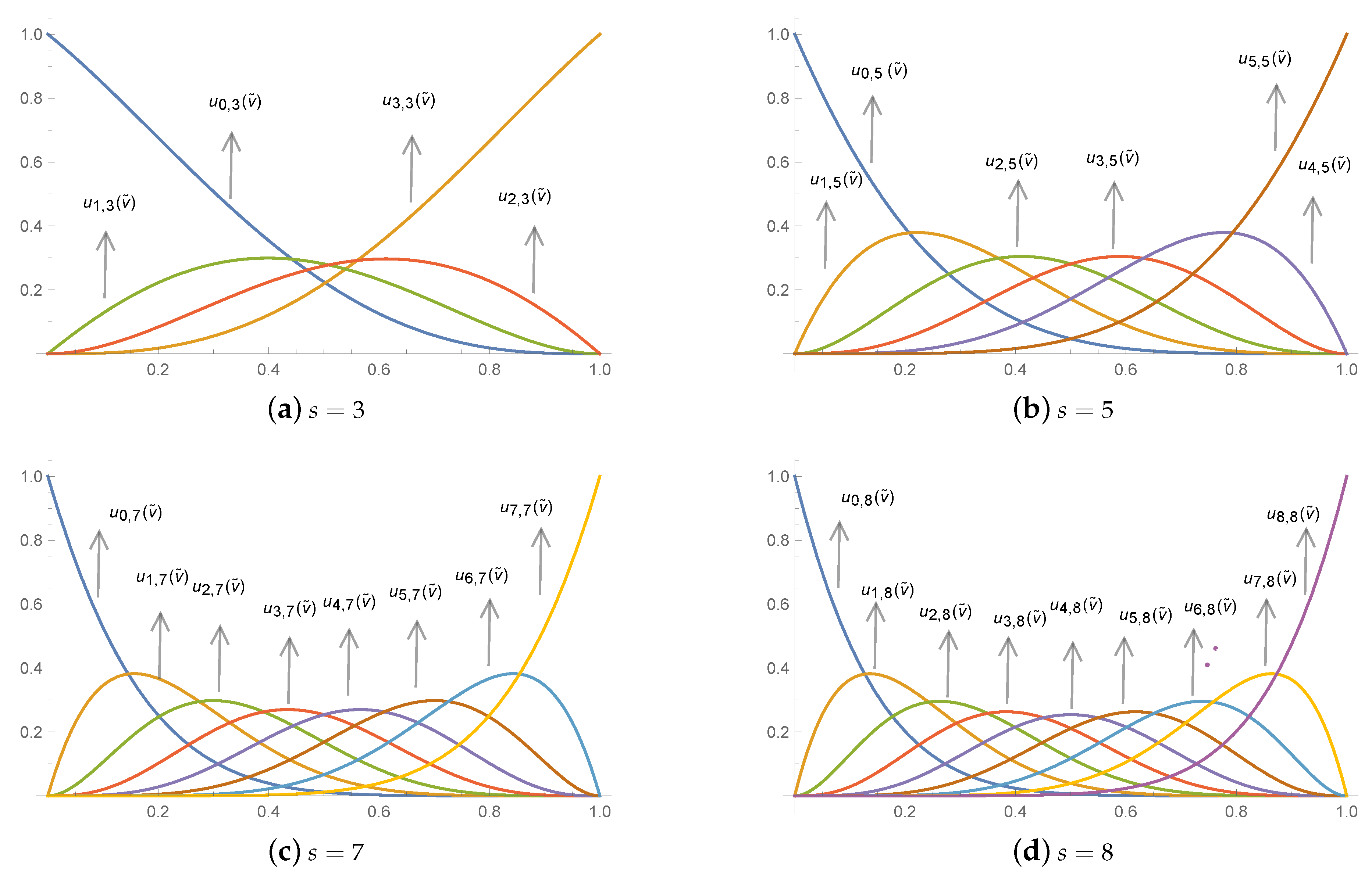
Let $\lambda ,\mu \in [0,3]$, for $\tilde{v}\in [0,1]$, then the following functions:

$$\left\{\begin{array}{c}{u}_{0,3}\left(\tilde{v}\right)={(1-\tilde{v})}^3(1+(2-\lambda )\tilde{v}),\hfill \\ u_{1,3}\left(\tilde{v}\right)=\tilde{v}{(1-\tilde{v})}^2(1+\lambda +\tilde{v}(2+\mu -2\lambda )),\hfill \\ u_{2,3}\left(\tilde{v}\right)={\tilde{v}}^2(1-\tilde{v})(3+\lambda -\mu +\tilde{v}(-2+2\mu -\lambda )),\hfill \\ u_{3,3}\left(\tilde{v}\right)={\tilde{v}}^3(3-\mu +\tilde{v}(\mu -2)).\hfill \end{array}\right.$$

(7)

are called the Bernstein-like basis functions of degree $s=3$.

Figure 1 displays the Bernstein-like basis functions graphs of degree $s=3,5,7,8$. Figure 2 shows the graph of cubic and quartic Bernstein-like basis functions with particular values of shape parameters. Thick, thin, dashed and dotted graphs correspond to $\lambda =0.5,1,1.5,2.1$ and $\mu =0.6,1.1,1.6,2.2$ respectively.

For the sake of conciseness, we will omit the independent variable and abbreviate $u_{l,s}\left(\tilde{v}\right)$, $U_{l,s}\left(\tilde{v}\right)$ to $u_{l,s}$, $U_{l,s}$, respectively. Furthermore, we shall use the notation $u_{ls}$, $U_{ls}$ for $u_{l,s}$,$U_{l,s}$, respectively, if there is no confusion, where $U_{l,s}$, $l=1,2,\dots ,s$ denotes the classical Bernstein basis function of degree s.

The CPU time(s) comparison of the proposed gBBF between existing basis functions [21,24,25] have been recorded in

Table 2. Computational comparisons of gBBF between existing Bernstein-like basis functions in terms of CPU time (s).

Degree s	Proposed gBBF	Samia et al. [21]	Sidra et al. [24]	Sidra et al. [25]
3	0.062500	0.203125	0.312500	0.15625
7	0.000000	0.015625	0.015625	0.015625
9	0.015625	0.046875	0.015625	0.046875
11	0.031250	0.156250	0.125000	0.062500
13	0.156250	0.546875	0.546875	0.328125
15	0.781250	1.937500	2.046880	1.859380

and

Table 3. Comparison of graphical outcomes of gBBF between existing Bernstein-like basis functions in terms of CPU time (s).

Degree s	Proposed gBBF	Samia et al. [21]	Sidra et al. [24]	Sidra et al. [25]
3	0.062500	0.203125	0.312500	0.15625
5	0.140625	0.265600	0.265600	0.50000
7	0.281250	0.843750	0.869375	1.04688
9	1.437500	3.347500	3.390630	3.20313
11	6.156250	14.32810	14.04690	13.1875
13	26.70130	62.15630	58.92190	49.8750
15	124.5000	269.4690	263.4380	210.578

for numerical computations and graphical display, respectively. It can be concluded that the proposed gBBFs are simpler, more straight-forward and more computationally economical than the existing basis functions.

Proposition 1.

The Bernstein-like basis functions can be expressed explicitly as:

$$\begin{array}{ccc}\hfill u_{l,s}& =& [\frac{{}^s{C}_l-2{(}^{s-3}{C}_{l-1}{-}^{s-3}{C}_{l-3})}{{}^s{C}_l}+\frac{{}^{s-2}{C}_{l-1}}{{}^s{C}_l}\lambda -\frac{{}^{s-2}{C}_{l-2}}{{}^s{C}_l}\mu -\frac{{}^{s-1}{C}_l}{{}^s{C}_l}\lambda \tilde{v}\hfill \\ & & +\frac{{}^{s-1}{C}_{l-1}}{{}^s{C}_l}\mu \tilde{v}+2\tilde{v}\frac{{(}^{s-2}{C}_l{-}^{s-2}{C}_{l-2})}{{}^s{C}_l}]{}^s{C}_l{\tilde{v}}^i{(1-\tilde{v})}^{s-l},\hfill \end{array}$$

(8)

where ${}^s{C}_l=\frac{s!}{l!(s-l)!}$ and $l=0,1,\dots ,s,s\ge 3$.

Proof. 

By induction on s. When $s=3$, it is simple to test the validity of basis functions given in Equation (7). Now, presume that the plan is worth for integer t such as $s=t$. When it is $s=t+1$, by recursive expression (6) and previous assumptions, for every $l=1,2,\dots ,t$, we obtain:

$$\begin{array}{ccc}\hfill u_{l,t+1}& =& [\frac{{}^t{C}_l-2{(}^{t-3}{C}_{l-1}{-}^{t-3}{C}_{l-3})}{{}^t{C}_l}+\frac{{}^{t-2}{C}_{l-1}}{{}^t{C}_l}\lambda -\frac{{}^{t-2}{C}_{l-2}}{{}^t{C}_l}\mu -\frac{{}^{t-1}{C}_l}{{}^t{C}_l}\lambda \tilde{v}\hfill \\ & & +\frac{{}^{t-1}{C}_{l-1}}{{}^t{C}_l}\mu \tilde{v}+2\tilde{v}\frac{{}^{t-2}{C}_l{-}^{t-2}{C}_{l-2}}{{}^t{C}_l}]{}^t{C}_l{\tilde{v}}^l{(1-\tilde{v})}^{t-i}\hfill \\ & & +[\frac{{}^t{C}_{l-1}-2{(}^{t-3}{C}_{l-2}{-}^{t-3}{C}_{l-4})}{{}^t{C}_{l-1}}+\frac{{}^{t-2}{C}_{l-2}}{{}^t{C}_{l-1}}\lambda -\frac{{}^{t-2}{C}_{l-3}}{{}^t{C}_{l-1}}\mu \hfill \\ & & -\frac{{}^{t-1}{C}_{l-1}}{{}^t{C}_{l-1}}\lambda \tilde{v}+\frac{{}^{t-1}{C}_{l-2}}{{}^t{C}_{l-1}}\mu \tilde{v}+2\tilde{v}\frac{{}^{t-2}{C}_{l-1}{-}^{t-2}{C}_{l-3}}{{}^t{C}_{l-1}}]{}^t{C}_{l-1}{\tilde{v}}^l{(1-\tilde{v})}^{t-l+1}\hfill \\ & =& [({(}^t{C}_l{+}^t{C}_{l-1})-2{(}^{t-3}{C}_{l-1}{+}^{t-3}{C}_{l-2})+2{(}^{t-3}{C}_{l-3}{+}^{t-3}{C}_{l-4}))+{\lambda }^{t-2}{C}_{l-1}\hfill \\ & & +{\lambda }^{t-2}{C}_{l-2}{)-\mu {(}^{t-2}{C}_{l-2}{+}^{t-2}{C}_{l-3})-\lambda \tilde{v}{(}^{t-1}{C}_l{+}^{t-1}{C}_{l-1})+\mu \tilde{v}(}^{t-1}{C}_{l-1}\hfill \\ & & +\mu \tilde{v}{(}^{t-1}{C}_{l-2}))+2\tilde{v}{(}^{t-2}{C}_l{+}^{t-2}{C}_{l-1})-2\tilde{v}{(}^{t-2}{C}_{l-2}{+}^{t-2}{C}_{l-3})]{\tilde{v}}^l{(1-\tilde{v})}^{t-l+1}\hfill \\ & =& [\frac{{}^{t+1}{C}_l-2{(}^{t-2}{C}_{l-1}{-}^{t-2}{C}_{l-3})}{{}^{t+1}{C}_l}+\frac{{}^{t-1}{C}_{l-1}}{{}^{t+1}{C}_l}\lambda -\frac{{}^{t-1}{C}_{l-2}}{{}^{t+1}{C}_l}\mu \hfill \\ & & -\frac{{}^t{C}_l}{{}^{t+1}{C}_l}\lambda \tilde{v}+\frac{{}^t{C}_{l-1}}{{}^{t+1}{C}_l}\mu \tilde{v}+2\tilde{v}\frac{{}^{t-1}{C}_l{-}^{t-1}{C}_{l-2}}{{}^{t+1}{C}_l}]{}^{t+1}{C}_l{\tilde{v}}^l{(1-\tilde{v})}^{t-l+1}.\hfill \end{array}$$

For $l=0$ in (6), we have:

$$\begin{array}{ccc}\hfill u_{0,t+1}& =& (1-\tilde{v})u_{0,t}\hfill \\ & =& [\frac{{}^t{C}_0-2{(}^{t-3}{C}_{-1}{-}^{t-3}{C}_{-3})}{{}^t{C}_0}+\frac{{}^{t-2}{C}_{-1}\lambda }{{}^t{C}_0}-\frac{{}^{T-2}{C}_{-2}\mu }{{}^t{C}_0}-\frac{{}^{t-1}{C}_0\lambda \tilde{v}}{{}^t{C}_0}+\frac{{}^{t-1}{C}_{-1}\mu \tilde{v}}{{}^t{C}_0}\hfill \\ & & +\frac{2\tilde{v}{(}^{t-2}{C}_0{-}^{t-2}{C}_{0-2})}{{}^t{C}_0}]{}^t{C}_0{\tilde{v}}^0{(1-\tilde{v})}^t\hfill \\ & =& [\frac{{}^{s+1}{C}_0-2{(}^{s-2}{C}_{-1}{-}^{s-2}{C}_{-3})}{{}^{s+1}{C}_0}+\frac{{}^{s-1}{C}_{-1}\lambda }{{}^{s+1}{C}_0}-\frac{{}^{s-1}{C}_{-2}\mu }{{}^{s+1}{C}_0}-\frac{{}^s{C}_0\lambda \tilde{v}}{{}^{s+1}{C}_0}+\frac{{}^s{C}_{-1}\mu \tilde{v}}{{}^{s+1}{C}_0}\hfill \\ & & +\frac{2\tilde{v}{(}^{s-1}{C}_0{-}^{s-1}{C}_{-2})}{{}^{s+1}{C}_0}]{}^{s+1}{C}_0{\tilde{v}}^0{(1-\tilde{v})}^{s+1}.\hfill \end{array}$$

The evidence for the $l=t+1$ proves the result. □

Proposition 2.

The Bernstein-like basis functions can be displayed as a linear combined effect of the classical Bernstein basis functions of degree s and $s+1$, i.e.,:

$$\begin{array}{ccc}\hfill u_{l,s}\left(\tilde{v}\right)& =& U_{l,s}\left(\tilde{v}\right)+\frac{2{(}^{s-2}{C}_l{-}^{s-2}{C}_{l-2}{+}^{s-3}{C}_{l-3}{-}^{s-3}{C}_l)}{{}^{s+1}{C}_{l+1}}{U}_{l+1,s+1}\left(\tilde{v}\right)\hfill \\ & & +\frac{2{(}^{s-3}{C}_{l-3}{-}^{s-3}{C}_{l-1})}{{}^{s+1}{C}_l}{U}_{l,s+1}\left(\tilde{v}\right)+\lambda \frac{{(}^{s-2}{C}_{l-1}{-}^{s-1}{C}_l)}{{}^{s+1}{C}_{l+1}}{U}_{l+1,s+1}\left(\tilde{v}\right)\hfill \\ & & +\lambda \frac{{}^{s-2}{C}_{l-1}}{{}^{s+1}{C}_l}{U}_{l,s+1}\left(\tilde{v}\right)+\mu \frac{{}^{s-1}{C}_{l-1}{-}^{s-2}{C}_{l-2}}{{}^{s+1}{C}_{l+1}}{U}_{l+1,s+1}\left(\tilde{v}\right)+\mu -\frac{{}^{s-2}{C}_{l-2}}{{}^{s+1}{C}_l}{U}_{l,s+1}\left(\tilde{v}\right).\hfill \end{array}$$

Proof. 

Simple algebraic manipulation of the above proposition yields:

$$\begin{array}{ccc}\hfill u_{l,s}\left(\tilde{v}\right)& =& [1+2\frac{{}^{s-3}{C}_{l-3}{-}^{s-3}{C}_{l-1}}{{}^s{C}_l}+2\tilde{v}\frac{{}^{s-2}{C}_l{-}^{s-2}{C}_{l-2}}{{}^s{C}_l}+\lambda (\frac{{}^{s-2}{C}_{l-1}}{{}^s{C}_l}-\frac{{}^{s-1}{C}_l}{{}^s{C}_l}\tilde{v})\hfill \\ & & +\mu (-\frac{{}^{s-2}{C}_{l-2}}{{}^s{C}_l}+\frac{{}^{s-1}{C}_{l-1}}{{}^s{C}_l}\tilde{v})]{}^s{C}_l{\tilde{v}}^l{(1-\tilde{v})}^{s-l}\hfill \\ & =& [1+\left(2\frac{{}^{s-2}{C}_l{-}^{s-2}{C}_{l-2}{+}^{s-3}{C}_{l-3}{-}^{s-3}{C}_{l-1}}{{}^s{C}_l}\right)\tilde{v}+2(1-\tilde{v})\frac{{}^{s-3}{C}_{l-3}{-}^{s-3}{C}_{l-1}}{{}^s{C}_l}\hfill \\ & & +\lambda \left[\left(\tilde{v}\frac{{}^{s-2}{C}_{l-1}{-}^{s-1}{C}_l}{{}^s{C}_l}\right)+\frac{{}^{s-2}{C}_{l-1}}{{}^s{C}_l}(1-\tilde{v})\right]+\mu [\left(\tilde{v}\frac{{}^{s-1}{C}_{l-1}{-}^{s-2}{C}_{l-2}}{{}^s{C}_l}\right)\hfill \\ & & -\frac{{}^{s-2}{C}_{l-2}}{{}^s{C}_l}(1-\tilde{v})\left]\right]{}^s{C}_l{\tilde{v}}^l{(1-\tilde{v})}^{s-l}\hfill \\ & =& U_{l,s}\left(\tilde{v}\right)+2\frac{{}^{s-2}{C}_l{-}^{s-2}{C}_{l-2}{+}^{s-3}{C}_{l-3}{-}^{s-3}{C}_l}{{}^{s+1}{C}_{l+1}}{U}_{l+1,s+1}\left(\tilde{v}\right)\hfill \\ & & +\frac{2{(}^{s-3}{C}_{l-3}{-}^{s-3}{C}_{l-1})}{{}^{s+1}{C}_l}{U}_{l,s+1}\left(\tilde{v}\right)+\lambda \frac{{}^{s-2}{C}_{l-1}{-}^{s-1}{C}_l}{{}^{s+1}{C}_{l+1}}{U}_{l+1,s+1}\left(\tilde{v}\right)\hfill \\ & & +\lambda \frac{{}^{s-2}{C}_{l-1}}{{}^{s+1}{C}_l}{U}_{l,s+1}\left(\tilde{v}\right)+\mu \frac{{}^{s-1}{C}_{l-1}{-}^{s-2}{C}_{l-2}}{{}^{s+1}{C}_{l+1}}{U}_{l+1,s+1}\left(\tilde{v}\right)-\mu \frac{{}^{s-2}{C}_{l-2}}{{}^{s+1}{C}_l}{U}_{l,s+1}\left(\tilde{v}\right).\hfill \end{array}$$

Therefore, the proposition persists. □

3.2. Properties of the Bernstein-like Basis Functions

In this section, some geometric properties of Bernstein-like basis functions are discussed as follows:

1.

Degeneracy: If $\lambda ,\mu =2,$ $u_{l,s}\left(\tilde{v}\right)=U_{l,s}\left(\tilde{v}\right)(l=0,1,\cdots ,s;s\ge 2)$. That is, the Bernstein-like basis functions of the degree s with the parameters $\lambda ,\mu =2$ are only the standard Bernstein basis functions of the degree s.

Proof. 

Put $\lambda ,\mu =2$ in (7) to obtain:

$$\left\{\begin{array}{c}{u}_{0,3}\left(\tilde{v}\right)={(1-\tilde{v})}^3,\hfill \\ u_{1,3}\left(\tilde{v}\right)=3\tilde{v}{(1-\tilde{v})}^2,\hfill \\ u_{2,3}\left(\tilde{v}\right)=3{\tilde{v}}^2(1-\tilde{v}),\hfill \\ u_{3,3}\left(\tilde{v}\right)={\tilde{v}}^3,\hfill \end{array}\right.$$

the classical cubic Bernstein polynomials.

For $s=4$ in Equation (8), yield the quartic Bernstein-like basis functions as follows:

Let $\lambda ,\mu \in [0,3]$, for $\tilde{v}\in [0,1]$:

$$\left\{\begin{array}{c}{u}_{0,4}\left(\tilde{v}\right)={(1-\tilde{v})}^4(1+(2-\lambda )\tilde{v}),\hfill \\ u_{1,4}\left(\tilde{v}\right)=\tilde{v}{(1-\tilde{v})}^3(2+\lambda +\tilde{v}(4+\mu -3\lambda )),\hfill \\ u_{2,4}\left(\tilde{v}\right)={\tilde{v}}^2{(1-\tilde{v})}^2(4+2\lambda -\mu +\tilde{v}(3\mu -3\lambda )),\hfill \\ u_{3,4}\left(\tilde{v}\right)={\tilde{v}}^3(1-\tilde{v})(6+\lambda -2\mu +\tilde{v}(-4+3\mu -\lambda )),\hfill \\ u_{4,4}\left(\tilde{v}\right)={\tilde{v}}^4(3-\mu +\tilde{v}(\mu -2)).\hfill \end{array}\right.$$

(9)

Put $\lambda ,\mu =2$ in (9) to obtain

$$\left\{\begin{array}{c}{u}_{0,4}\left(\tilde{v}\right)={(1-\tilde{v})}^4,\hfill \\ u_{1,4}\left(\tilde{v}\right)=4\tilde{v}{(1-\tilde{v})}^3,\hfill \\ u_{2,4}\left(\tilde{v}\right)=6{\tilde{v}}^2{(1-\tilde{v})}^2,\hfill \\ u_{3,4}\left(\tilde{v}\right)=4{\tilde{v}}^3(1-\tilde{v}),\hfill \\ u_{4,4}\left(\tilde{v}\right)={\tilde{v}}^4,\hfill \end{array}\right.$$

the classical quartic Bernstein polynomials.

This proof is also valid for higher degrees upto s. □

2.

Non-negativity: When $\lambda ,\mu \in [0,3]$, $u_{l,s}\left(\tilde{v}\right)\ge 0(l=0,1,\dots ,s;s\ge 2)$.

Proof. 

By induction for s. If $s=2$, we will rewrite the Bernstein-like basis functions as:

$$\left\{\begin{array}{c}{u}_{0,2}\left(\tilde{v}\right)=U_{0,3}\left(\tilde{v}\right)+\left(\frac{3-\lambda }{3}\right)U_{1,3}\left(\tilde{v}\right),\hfill \\ u_{1,2}\left(\tilde{v}\right)=\frac{\lambda }{3}{U}_{1,3}\left(\tilde{v}\right)+\left(\frac{\mu }{3}\right)U_{2,3}\left(\tilde{v}\right),\hfill \\ u_{2,2}\left(\tilde{v}\right)=U_{3,3}\left(\tilde{v}\right)+\left(\frac{\mu -3}{3}\right)U_{2,3}\left(\tilde{v}\right).\hfill \end{array}\right.$$

(10)

Obviously, when $\lambda ,\mu \in [0,3]$, we have $3-\lambda ,3-\mu \ge 0$, $\lambda ,\mu \ge 0$. In fact, let us recognize that the cubic Bernstein-like basis functions $U_{l,3}(l=0,1,2,3)$ are non-negative. The Bernstein-like basis functions of degree 2 are therefore non-negative.

Now, suppose that the Bernstein-like basis functions of degree t are non-negative. We obtain $s=t+1$ from Equation (6):

$$u_{l,t+1}\left(\tilde{v}\right)=(1-\tilde{v})u_{l,t}\left(\tilde{v}\right)+\tilde{v}{u}_{l-1,t}\left(\tilde{v}\right),(l=0,1,\dots ,t+1).$$

(11)

By our inductive hypothesis and the fact that $1-\tilde{v}\ge 0$, $\tilde{v}\ge 0$, we can conclude that the Bernstein-like basis functions of degree $s=t+1$ are non-negative. □

3.

Normalization: For $s\ge 2,$ ${\sum }_{l=0}^s{u}_{l,s}\left(\tilde{v}\right)=1$.

Proof. 

Through induction to s, as we obtain $s=2,$ from (10)

$$\sum _{l=0}^2{u}_{l,2}\left(\tilde{v}\right)=\sum _{i=0}^3{U}_{i,3}\left(\tilde{v}\right)=1.$$

Now, assume that the equality holds for $s=t$. Then, when $s=t+1,$ according to the recursive Formula (6) and the inductive hypothesis, we have:

$$\begin{array}{ccc}\hfill \sum _{l=0}^{t+1}{u}_{l,t+1}\left(\tilde{v}\right)& =& \sum _{l=0}^{t+1}[(1-\tilde{v})u_{l,t}\left(\tilde{v}\right)+\tilde{v}{u}_{l-1,t}\left(\tilde{v}\right)],\hfill \\ & =& (1-\tilde{v})\sum _{l=0}^t{u}_{l,t}\left(\tilde{v}\right)+\tilde{v}\sum _{l-1=0}^t{u}_{l-1,t}\left(\tilde{v}\right),\hfill \\ & =& (1-\tilde{v})\left(1\right)+\tilde{v}\left(1\right),\hfill \\ & =& 1.\hfill \end{array}$$

□

4.

Symmetry:

$$u_{l,s}(1-\tilde{v})=u_{s-i,s}\left(\tilde{v}\right),l=0,1,\dots n,\tilde{v}\in [0,1].$$

Proof. 

By induction on s, when $s=3$ from (7) and the symmetry of cubic Bernstein-like basis functions

$$u_{l,3}(1-\tilde{v})=u_{3-l,s}\left(\tilde{v}\right),l=0,1,2,3,\tilde{v}\in [0,1].$$

We assume that Bernstein-like basis functions of degree 3 are symmetrical.

Now, assume that the Bernstein-like basis functions of order t are symmetrical. Then, from the inductive hypothesis and recursive Formula (6), we have:

$$\begin{array}{ccc}\hfill u_{l,t+1}(1-\tilde{v})& =& (1-\tilde{v})u_{l-1,t}(1-\tilde{v})+\tilde{v}{u}_{l,t}(1-\tilde{v})\hfill \\ & =& (1-\tilde{v})u_{t+1-l,r}\left(\tilde{v}\right)+\tilde{v}{u}_{t+1-l-1,t}\left(\tilde{v}\right)\hfill \\ & =& (1-\tilde{v})u_{t+1-l,t}\left(\tilde{v}\right)+\tilde{v}{u}_{t-l,t}\left(\tilde{v}\right)\hfill \\ & =& u_{t+1-l,t+1}\left(\tilde{v}\right).\hfill \end{array}$$

□

5.

Property at the end points: For $l=0,1,\dots ,s,(s\ge 2)$:

$$u_{l,s}\left(0\right)=\left\{\begin{array}{c}1,l=0,\hfill \\ 0,l\ne 0.\hfill \end{array}\right.$$

(12)

$$u_{l,s}\left(1\right)=\left\{\begin{array}{c}1,l=s,\hfill \\ 0,l\ne s.\hfill \end{array}\right.$$

(13)

Proof. 

By induction on s, if $s=2,$ the expression (5) can be obtained by simple calculation. Now, assume the above condition holds for $s=t$. When $s=t+1$ from recursive Formula (6) and the inductive hypothesis, we obtain:

$$\left\{\begin{array}{c}{u}_{l,t+1}\left(0\right)=u_{l,t}\left(0\right)=1,l=0,\hfill \\ u_{l,t+1}\left(0\right)=u_{l,t}\left(0\right)=0,l\ne 0,\hfill \end{array}\right.$$

(14)

and

$$\left\{\begin{array}{c}{u}_{l,t+1}\left(1\right)=u_{l-1,t}\left(1\right)=1,l=t+1,\hfill \\ u_{l,t+1}\left(0\right)=u_{l,t}\left(0\right)=0,l\ne t+1.\hfill \end{array}\right.$$

(15)

These show that the conclusion listed in (12) and (13) also holds for $s=t+1$. □

6.

Derivative at the corner points: For $l=0,1,\dots ,s;(s\ge 3)$:

$$u_{l,s}^{\prime }\left(0\right)=\left\{\begin{array}{cc}-(s-2+\lambda ),\hfill & l=0,\hfill \\ (s-2+\lambda ),\hfill & l=1,\hfill \\ 0,\hfill & \mathrm{other},\hfill \end{array}\right.$$

(16)

and

$$u_{l,s}^{\prime }\left(1\right)=\left\{\begin{array}{cc}-(s-2+\mu ),\hfill & l=s-1,\hfill \\ (s-2+\mu ),\hfill & l=s,\hfill \\ 0,\hfill & \mathrm{other}.\hfill \end{array}\right.$$

(17)

Proof. 

By induction on s, when $s=3$, differentiating (7):

$$\left\{\begin{array}{c}{u}_{0,3}^{\prime }\left(\tilde{v}\right)={(1-\tilde{v})}^2(-1+4v(-2+\lambda )-\lambda ),\hfill \\ u_{1,3}^{\prime }\left(\tilde{v}\right)=(\tilde{v}-1)(1+\lambda +\tilde{v}(1-7\lambda +2\mu +\tilde{v}(8\lambda -4(2+\mu )))),\hfill \\ u_{2,3}^{\prime }\left(\tilde{v}\right)=\tilde{v}(2(3+\lambda -\mu )+\tilde{v}(-15-6\lambda +4\tilde{v}(2+\lambda -2\mu )+9\mu )),\hfill \\ u_{3,3}^{\prime }\left(\tilde{v}\right)={\tilde{v}}^2(9+4\tilde{v}(-2+\mu )-3\mu ).\hfill \end{array}\right.$$

(18)

It is simple to infer from the above that the findings seen in (16) and (17) are $s=3$.

Now, presume that the consequence given in (16) and (17) is $s=t$ while $s=t+1$. From recursive Formula (6), we have:

$$u_{l,t+1}\left(\tilde{v}\right)=(1-\tilde{v})u_{l,t}\left(\tilde{v}\right)+\tilde{v}{u}_{l-1,t}\left(\tilde{v}\right),l=0,1,\dots ,t+1,\tilde{v}\in [0,1].$$

We obtain the following through differentiating one time:

$$u_{i,t+1}^{\prime }\left(\tilde{v}\right)=(1-\tilde{v})u_{l,t}^{\prime }\left(\tilde{v}\right)-u_{l,t}\left(\tilde{v}\right)+\tilde{v}{u}_{l-1,t}^{\prime }\left(\tilde{v}\right)+u_{l-1,t}\left(\tilde{v}\right).$$

(19)

Taking $\tilde{v}=0$ in (19):

$$u_{i,t+1}^{\prime }\left(0\right)=u_{l,t}^{\prime }\left(0\right)-u_{l,t}\left(0\right)+u_{l-1,t}\left(0\right).$$

(20)

By induction and the findings suggested in (12) and (13), we have the following inference:

If $l=0$ in (20), then:

$$u_{0,t+1}^{\prime }\left(\tilde{v}\right)=-(t-1+\lambda ).$$

If $l=1$ in (20), then:

$$u_{1,t+1}^{\prime }\left(\tilde{v}\right)=(t+\lambda -1).$$

If $l\ne 0$ and $l\ne 1$ in (20), then:

$$u_{L,t+1}^{\prime }\left(\tilde{v}\right)=0.$$

This conclusion shows that (16) holds for $n=t+1$. Similarly, we can prove the (17) for $(s=t+1)$. □

7.

Linear Independence:${\sum }_{l=0}^s{c}_l{u}_{l,s}\left(\tilde{v}\right)=0$ iff $c_i=0,l=0,1,\dots ,s;s\ge 2$.

Proof. 

Sufficient condition is clear, and we shall show the requirement by induction as follows:

First of all, we find the linear combination to be trivial:

$$\begin{array}{ccc}\hfill \sum _{l=0}^2{c}_i{u}_{l,2}& =& 0\hfill \\ \hfill c_0{u}_{0,2}+c_1{u}_{1,2}+c_2{u}_{2,2}& =& 0.\hfill \end{array}$$

Substituting (10) into above equation, we obtain:

$$\begin{array}{ccc}\hfill & & c_0(U_{0,3}\left(\tilde{v}\right)+\left(\frac{3-\lambda }{3}\right)U_{1,3}\left(\tilde{v}\right))+c_1(\frac{\lambda }{3}{U}_{1,3}\left(\tilde{v}\right)+\left(\frac{\mu }{3}\right)U_{2,3}\left(\tilde{v}\right))\hfill \\ \hfill & & +c_2(U_{3,3}\left(\tilde{v}\right)+\left(\frac{\mu -3}{3}\right)U_{2,3}\left(\tilde{v}\right))=0\hfill \end{array}$$

$$c_0{U}_{0,3}\left(\tilde{v}\right)+U_{1,3}\left(\tilde{v}\right)(c_0\frac{3-\lambda }{3}+c_1\frac{\lambda }{3})+U_{2,3}\left(\tilde{v}\right)(c_1\frac{\mu }{3}+c_2\frac{\mu -3}{3})+c_3{U}_{3,3}\left(\tilde{v}\right)=0.$$

(21)

By comparing coefficients, we obtain:

$$\left\{\begin{array}{cc}{c}_0\hfill & =0,\hfill \\ c_0\frac{3-\lambda }{3}+c_1\frac{\lambda }{3}\hfill & =0,\hfill \\ c_1\frac{\mu }{3}+c_2\frac{\mu -3}{3}\hfill & =0,\hfill \\ c_3\hfill & =0.\hfill \end{array}\right.$$

Upon any simplification, we receive from the linear freedom of the cubic Bernstein basis function: $c_l=0,l=0,1,2$.

It ensures that the Bernstein-like basis functions of the degree 2 is linearly independent.

Assume the Bernstein-like basis functions of degree t are linearly independent. After that, we are going to prove that Bernstein-like basis functions are linearly independent of degree $t+1$.

Let us consider the linear combination:

$$\sum _{l=0}^{t+1}{a}_i{u}_{l,t+1}=0,$$

(22)

where $c_l\in R,l=0,1,\dots ,t+1$. Substituting recursive Formula (6) in the above equation and rearranging it, we obtain:

$$(1-\tilde{v})\sum _{l=0}^{t+1}{c}_i{u}_{l,t}\left(\tilde{v}\right)+\tilde{v}\sum _{l=0}^{t+1}{c}_l{u}_{l-1,t}\left(\tilde{v}\right)=0.$$

(23)

Because $\tilde{v}$ is an arbitrary value in the interval $[0,1],$ from the above equation, we obtain:

$$\sum _{l=0}^{t+1}{c}_i{u}_{l,t}\left(\tilde{v}\right)=0,$$

(24)

and

$$\sum _{l=0}^{t+1}{c}_i{u}_{l-1,t}\left(\tilde{v}\right).$$

(25)

Notice that $u_{a,b}=0$ if $a=-1$ or $a>b$. We obtain our inductive hypothesis along with (24), $c_l=0,l=0,1,\dots ,t$. Together with (25), we obtain $c_l=0,l=1,2,\dots ,t+1$. Synthesizing the above conclusion, we deduce that $c_l=0,l=0,1,\dots ,t+1$. This indicates that the Bernstein-like basis functions of degree $t+1$ are linearly independent. □

3.3. Construction and Properties of the Bézier-like Curve

Definition 4.

Given control points $V_l\in R^e(e=2,3;l=0,1,\dots ,s;s\ge 2)$, the expression:

$$P\left(\tilde{v}\right)=\sum _{l=0}^s{u}_{l,s}\left(\tilde{v}\right)V_l,\tilde{v}\in [0,1]$$

(26)

is called the Bézier-like curve of degree s, where $u_{l,s}\left(\tilde{v}\right)(l=0,1,\dots ,s)$ are the Bernstein-like basis functions.

Proposition 3.

The Bézier-like curve can be represented by linearly combining the classical Bézier curve with the degree s and $s+1$, as follows:

$$p_s\left(\tilde{v}\right)=u_s\left(\tilde{v}\right)+u_{s+1}\left(\tilde{v}\right)+\lambda {\tilde{v}}_{s+1}\left(\tilde{v}\right)+\mu {\widehat{v}}_{s+1}\left(\tilde{v}\right),$$

(27)

where,

$$u_s\left(\tilde{v}\right)=\sum _{l=0}^s{U}_{l,s}\left(\tilde{v}\right)V_l.$$

It is the Bézier curve of degree s, which has the same control points as the Bézier curve. The following expression:

$$p_s\left(\tilde{v}\right)=\sum _{l=0}^s{u}_{l,s}\left(\tilde{v}\right)V_l,$$

is the Bézier-like curve of degree s. The expression:

$$u_{s+1}\left(\tilde{v}\right)=\sum _{l=0}^{s+1}{U}_{l,s+1}\left(\tilde{v}\right)R_l,$$

is a Bézier curve of degree $s+1$, the control points of which are calculated according to the aforementioned:

$$R_l=2[\frac{{}^{s-2}{C}_{l-1}{-}^{s-2}{C}_{l-3}{+}^{s-3}{C}_{l-4}{-}^{s-3}{C}_{l-1}}{{}^{s+1}{C}_l}{V}_{l-1}+\frac{{}^{s-3}{C}_{l-3}{-}^{s-3}{C}_{l-1}}{{}^{s+1}{C}_l}{V}_l]$$

(28)

The expression:

$${\tilde{f}}_{s+1}\left(\tilde{v}\right)=\sum _{l=0}^{s+1}{U}_{l,s+1}\left(\tilde{v}\right)Q_l,$$

is a Bézier curve of degree $s+1$, the control points of which are calculated according to the aforementioned:

$$Q_l=\frac{{}^{s-2}{C}_{l-2}{-}^{s-1}{C}_{l-1}}{{}^{s+1}{C}_l}{V}_{l-1}+\frac{{}^{s-2}{C}_{l-1}}{{}^{s+1}{C}_l}{V}_l$$

(29)

and the expression:

$${\widehat{f}}_{s+1}\left(\tilde{v}\right)=\sum _{l=0}^{s+1}{U}_{l,s+1}\left(\tilde{v}\right)P_l$$

is also thre Bézier curve of degree $s+1$, the control points of which are calculated according to the aforementioned:

$$P_l=\frac{{}^{s-1}{C}_{l-2}{-}^{s-2}{C}_{l-3}}{{}^{s+1}{C}_l}{V}_{l-1}+\frac{{}^{s-2}{C}_{l-2}}{{}^{s+1}{C}_l}{V}_l.$$

(30)

Proof. 

From Proposition (2), we obtain:

$$\begin{array}{ccc}\hfill u_{l,s}\left(\tilde{v}\right)& =& [1+2\frac{{}^{s-3}{C}_{l-3}{-}^{s-3}{C}_{l-1}}{{}^s{C}_l}+2\tilde{v}\frac{{}^{s-2}{C}_l{-}^{s-2}{C}_{l-2}}{{}^s{C}_l}+\lambda (\frac{{}^{s-2}{C}_{l-1}}{{}^s{C}_l}-\frac{{}^{s-1}{C}_l}{{}^s{C}_l}\tilde{v})\hfill \\ & & +\mu (-\frac{{}^{s-2}{C}_{l-2}}{{}^s{C}_l}+\frac{{}^{s-1}{C}_{l-1}}{{}^s{C}_l}\tilde{v}){]}^s{C}_l{\tilde{v}}^l{(1-\tilde{v})}^{s-l}.\hfill \end{array}$$

(31)

Applying the definition of Bézier-like curve on (31), we obtain:

$$\begin{array}{ccc}\hfill p_s\left(\tilde{v}\right)& =& \sum _{l=0}^s{U}_{l,s}\left(\tilde{v}\right)V_l+\sum _{l=0}^{s}2\frac{{}^{s-2}{C}_l{-}^{s-2}{C}_{l-2}{+}^{s-3}{C}_{l-3}{-}^{s-3}{C}_l}{{}^{s+1}{C}_{l+1}}{U}_{l+1,s+1}\left(\tilde{v}\right)V_l\hfill \\ & & +\sum _{l=0}^{s}2\frac{{}^{s-3}{C}_{l-3}{-}^{s-3}{C}_{l-1}}{{}^{s+1}{C}_l}{U}_{l,s+1}\left(\tilde{v}\right)V_l+\sum _{l=0}^s\lambda \frac{{}^{s-2}{C}_{l-1}{-}^{s-1}{C}_l}{{}^{s+1}{C}_{l+1}}{U}_{l+1,s+1}\left(\tilde{v}\right)V_l\hfill \\ & & +\sum _{l=0}^s\lambda \left(\frac{{}^{s-2}{C}_{l-1}}{{}^{s+1}{C}_l}\right)U_{l,s+1}\left(\tilde{v}\right)V_l+\sum _{l=0}^s\mu \frac{{}^{s-1}{C}_{l-1}{-}^{s-2}{C}_{l-2}}{{}^{s+1}{C}_{l+1}}{U}_{l+1,s+1}\left(\tilde{v}\right)V_l\hfill \\ & & +\sum _{l=0}^s\mu (-\frac{{}^{s-2}{C}_{l-2}}{{}^{s+1}{C}_l})U_{l,s+1}\left(\tilde{v}\right)V_l\hfill \\ & =& \sum _{l=0}^s{U}_{l,s}\left(\tilde{v}\right)V_l+\sum _{l=1}^{s+1}2\frac{{}^{s-2}{C}_{l-1}{-}^{s-2}{C}_{l-3}{+}^{s-3}{C}_{l-4}{-}^{s-3}{C}_{l-1}}{{}^{s+1}{C}_l}{U}_{l,s+1}\left(\tilde{v}\right)V_{l-1}\hfill \\ & & +\sum _{l=0}^{s}2\frac{{}^{s-3}{C}_{l-3}{-}^{s-3}{C}_{l-1}}{{}^{s+1}{C}_l}{U}_{l,s+1}\left(\tilde{v}\right)V_l+\sum _{l=1}^{s+1}\lambda \frac{{}^{s-2}{C}_{l-2}{-}^{s-1}{C}_{l-1}}{{}^{s+1}{C}_l}{U}_{l,s+1}\left(\tilde{v}\right)V_{l-1}\hfill \\ & & +\sum _{l=0}^s\lambda \left(\frac{{}^{s-2}{C}_{l-1}}{{}^{s+1}{C}_l}\right)U_{l,s+1}\left(\tilde{v}\right)V_l+\sum _{l=1}^{s+1}\mu \frac{{}^{s-1}{C}_{l-2}{-}^{s-2}{C}_{l-3}}{{}^{s+1}{C}_l}{U}_{l,s+1}\left(\tilde{v}\right)V_{l-1}\hfill \\ & & +\sum _{l=0}^s\mu (-\frac{{}^{s-2}{C}_{l-2}}{{}^{s+1}{C}_l})U_{l,s+1}\left(\tilde{v}\right)V_l.\hfill \end{array}$$

Taking into consideration the idea that ${}^a{C}_b=0$ if $a>b$ or $b\ge 0$ or $a<0,$ after any simplification, we obtain:

$$\begin{array}{ccc}\hfill p_s\left(\tilde{v}\right)& =& \sum _{l=0}^s{U}_{l,s}\left(\tilde{v}\right)V_l+\sum _{l=0}^{s+1}2[\frac{{}^{s-2}{C}_{l-1}{-}^{s-2}{C}_{l-3}{+}^{s-3}{C}_{l-4}{-}^{s-3}{C}_{l-1}}{{}^{s+1}{C}_l}{V}_{l-1}\hfill \\ & & +\frac{{}^{s-3}{C}_{l-3}{-}^{s-3}{C}_{l-1}}{{}^{s+1}{C}_l}{V}_l]U_{l,s+1}\left(\tilde{v}\right)+\lambda \sum _{l=0}^{s+1}\frac{{}^{s-2}{C}_{l-2}{-}^{s-1}{C}_{l-1}}{{}^{s+1}{C}_l}{V}_{l-1}\hfill \\ & & +\frac{{}^{s-2}{C}_{l-1}}{{}^{s+1}{C}_l}{V}_l{U}_{l,s+1}\left(\tilde{v}\right)+\mu \sum _{l=0}^{s+1}\frac{{}^{s-1}{C}_{l-2}{-}^{s-2}{C}_{l-3}}{{}^{s+1}{C}_l}{V}_{l-1}+\frac{{}^{s-2}{C}_{l-2}}{{}^{s+1}{C}_l}{V}_l{U}_{l,s+1}\left(\tilde{v}\right)\hfill \\ & =& \sum _{l=0}^s{U}_{l,s}\left(\tilde{v}\right)V_l+\sum _{l=0}^{s+1}{U}_{l,s+1}\left(\tilde{v}\right)R_l+\lambda \sum _{l=0}^{s+1}{U}_{l,s+1}\left(\tilde{v}\right)Q_l+\mu \sum _{l=0}^{s+1}{U}_{l,s+1}\left(\tilde{v}\right)P_l,\hfill \end{array}$$

where $R_l,Q_l$ and $P_l$ are given in (28), (29) and (30), respectively. □

Along with the properties of the Bernstein-like basis functions and the concept of the classical Bézier curve, the following properties of the Bézier-like curve are easy to access:

1.

Convex hull property: The whole Bézier-like curve has to lie within the convex hull of its control polygon. This is implemented as the Bernstein-like basis functions being greater than zero and having a sum towards one.

2.

Geometric invariance: However, since $p\left(\tilde{v}\right)$ is an affine mixture of the control points, the Bézier-like curve geometry is distinct of coordinate system selection.

3.

Symmetry: Control points of the Bézier curve can be marked as $V_0,V_1,\dots ,V_s$ or $V_s,V_{s-1},\dots ,V_0$ without altering the structure of the curve. They are changed just in that they are reversed. When we do not understand the path of the curve, we have a curve:

$$\begin{gathered} P(\tilde{v};V_0,V_1,\dots ,V_s)={\sum }_{l=0}^s{u}_{l,s}\left(\tilde{v}\right)V_l={\sum }_{l=0}^s{u}_{s-l,s}(1-\tilde{v})V_l={\sum }_{l_1=0}^n{u}_{l_1,n}\left(\tilde{v}\right)V_{n-l_1} \\ =P(1-\tilde{v};V_s,V_{s-1},\dots ,V_0) \end{gathered}$$.

4.

Geometric property at the endpoints From the property and the derivative at the endpoints of the Bernstein-like basis functions, we obtain:

$P\left(0\right)=V_0$, $P\left(1\right)=V_s$, $P^{\prime }\left(0\right)=(s-2+\lambda )(V_1-V_0)$, $P^{\prime }\left(1\right)=(s-2+\mu )(V_s-V_{s-1})$

These imply that the Bézier-like curve interpolates at the endpoints and tangents at the end edges.

5.

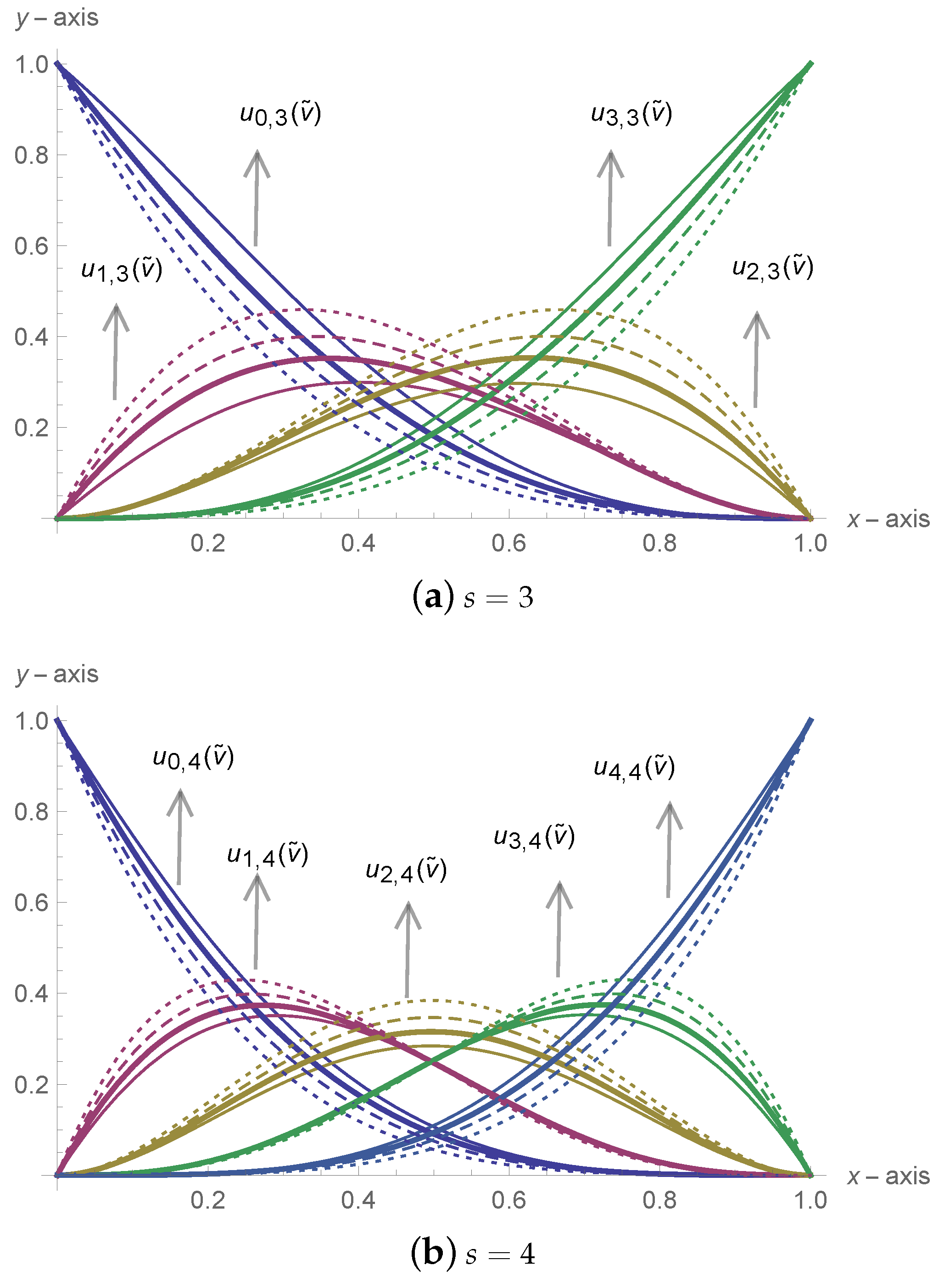
Shape adjustable property: With the control polygon, the form of the famous Bézier curve can be fully decided. Yet, this is not the case for the Bézier curve. Promising to fix the control polygon, the form of the Bézier-like curve can also be changed by adjusting the shape parameters.

Figure 3 displays four Bézier-like curve of degree 3 with similar control polygons with different shape parameters. From the figure, we can see that the Bézier-like curve introduces the control polygon by increasing the shape parameter. Besides that, since the Bézier-like curve seems to be just the classical Bézier curve when $\lambda ,\mu =2$.

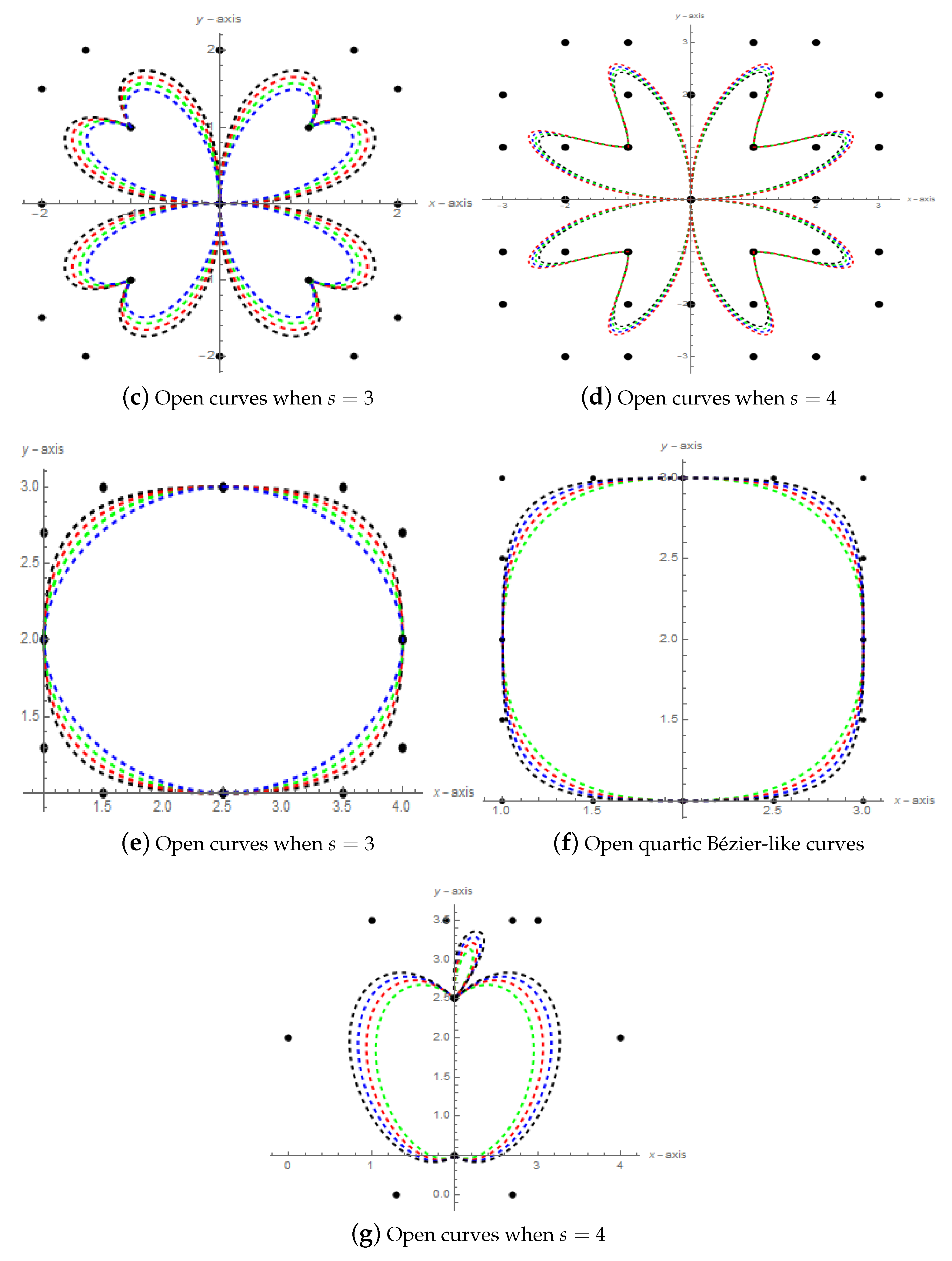
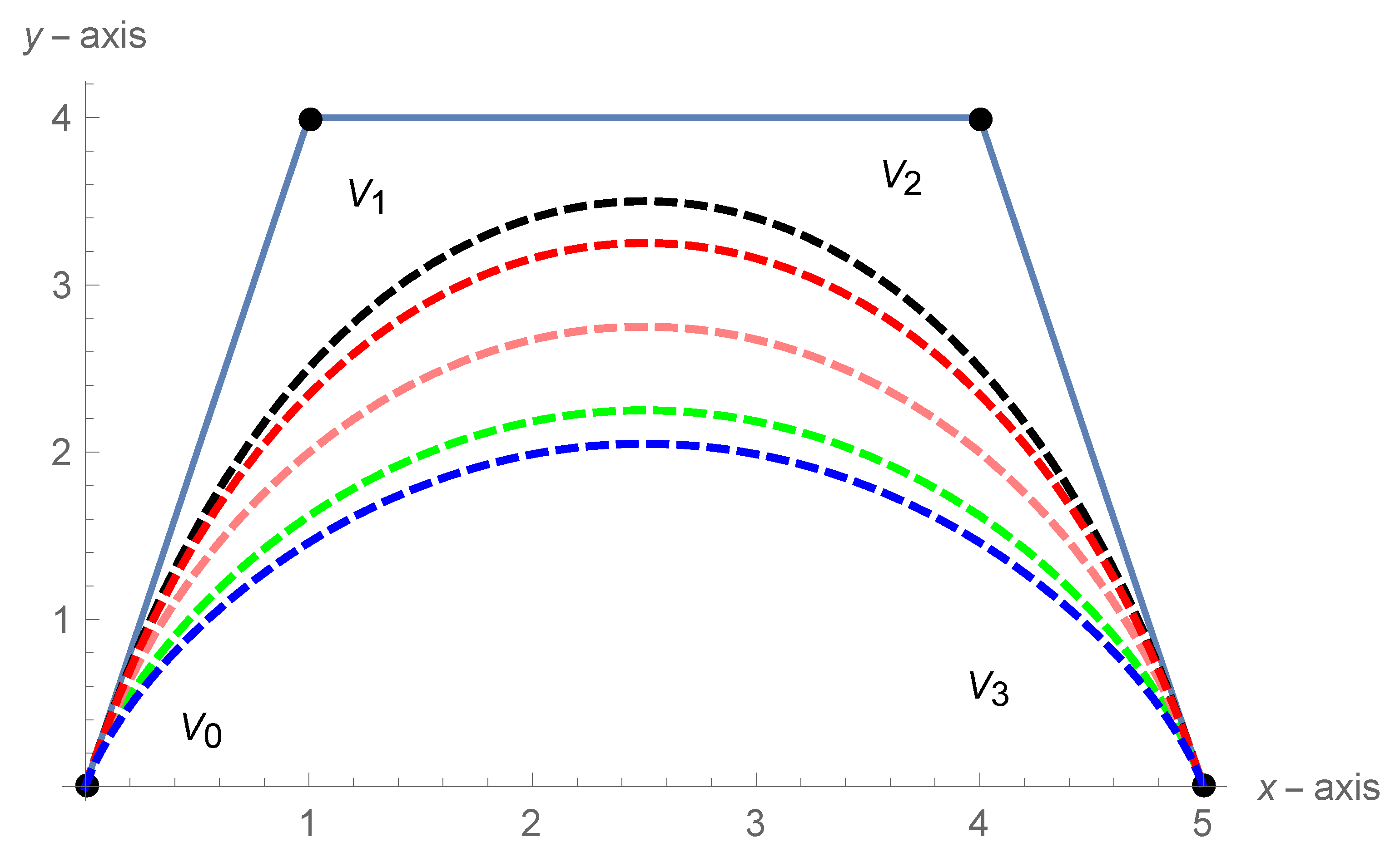
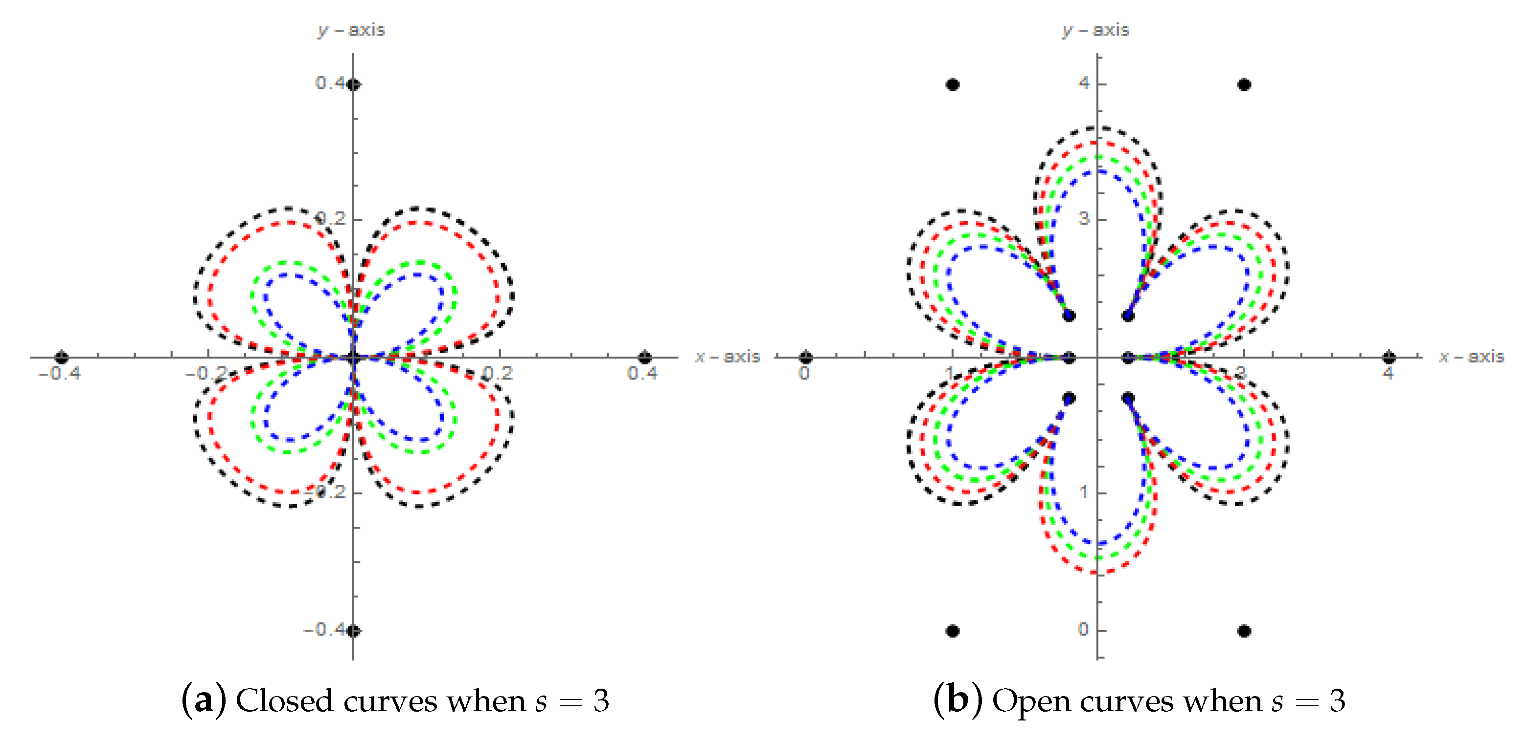
4. Open and Closed Curves

In this section, some free form open and closed curves are constructed with different value of shape parameters.

Here, we construct some free form curves by different degree of Bézier-like curves with different value of shape parameters. A curve is said to be closed curve if its first and last control points are equal otherwise it is open curve. Figure 4a shows a closed cubic Bézier-like curve with different value of shape parameters. In this figure, the blue curve is for $\lambda ,\mu =0.5,$ the green curve is for $\lambda ,\mu =1,$ the red curve is for $\lambda ,\mu =1.5$ and the black curve is for $\lambda ,\mu =2.5.$ Figure 4b,c,e show open cubic Bézier-like curves with the same shape parameters as mentioned above. Figure 4d shows an open quintic Bézier-like curve with with the same shape parameters as mentioned above. Figure 4f,g show open quartic Bézier-like curves with the same shape parameters as mentioned above. In Figure 4g, the leaf shows a closed cubic Bézier-like curve with different value of shape parameters.

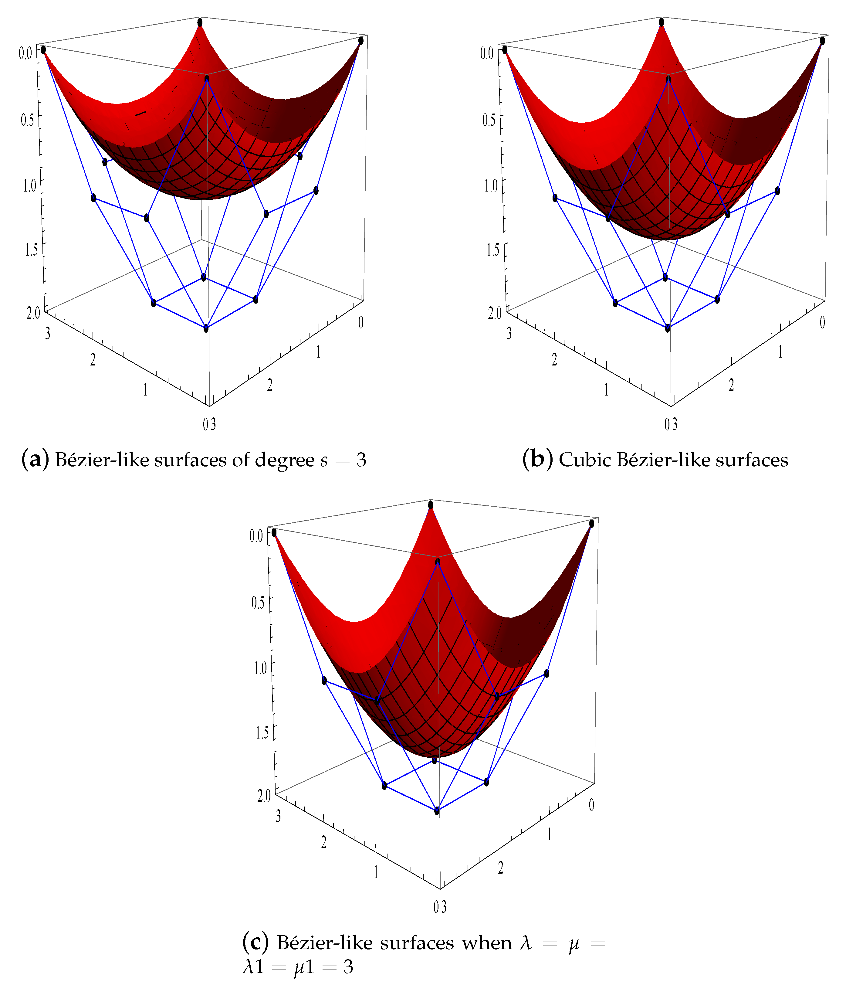
5. Development of Bézier-like Surfaces with Shape Parameters

Definition 5.

For the control point array $V_{l,l_1}\in R^3$, where $(l=0,1,2,\cdots ,s)$,$(l_1=0,1,2,\cdots ,s_1)$ and $s,s_1\ge 3,$ the tensor product Bézier-like surfaces can be defined as:

$$p(\tilde{v},\widetilde{v1};\mu ,\lambda ,\mu 1,\lambda 1)=\sum _{l=0}^s\sum _{l_1=0}^{s_1}{P}_{l,l_1}{u}_{l,s}\left(\tilde{v}\right)u_{l_1,s_1}\left(\widetilde{v1}\right)0\le \tilde{v},\widetilde{v1}\le 1,$$

(32)

with control points $V_{l,l_1},$ where $u_{l,s}\left(\tilde{v}\right)$ and $u_{l_1,s-1}\left(\widetilde{v1}\right)$ are Bernstein-like basis functions and $\lambda ,\mu$, and $\lambda 1,\mu 1$ are the shape parameters for the basis functions $u_{l,s}\left(\tilde{v}\right)$ and $u_{l_1,s_1}\left(\widetilde{v1}\right)$, respectively.

Remark 1.

The tensor product of Bézier-like surfaces has properties identical to the tensor product of the standard Bézier surfaces. By holding the control polygon unchanged, the structure of the Bézier-like surfaces may also be changed by adjusting the form parameters. This also has other properties close to the classic Bézier surface, such as the angular point interpolation nature, symmetry, form flexible property, convex hull asset, boundary property and affine invariance property.

Impact of Shape Parameters on Bézier-like Surfaces

Surfaces are simply the generalization of structures, the joint motion of two separate curves with the mesh points surfaces. However, much like curves, surfaces do display differences in their actions by changing various form parameters.

Example 1.

Assume a bi-cubic Bézier-like surface:

$$\begin{array}{cc}\hfill & p(\tilde{v},\tilde{v}1;\lambda ,\mu ,\lambda 1,\mu 1)\hfill \\ \hfill & =\sum _{l=0}^3\sum _{l_1=0}^3{Q}_{l,l_1}{u}_{l,3}\left(\tilde{v}\right)u_{l_1,3}\left(\widetilde{v1}\right)0\le \tilde{v},\widetilde{v1}\le 1\hfill \end{array}$$

(33)

Figure 5 demonstrates three Bézier-like $3\times 3$ degree surfaces with the same control points but different shape parameters. In Figure 5, the shape parameters $\lambda =0.5,1.8,3,\mu =0.6,1.9,3,\lambda 1=0.5,1.8,3$ and $\mu 1=0.6,1.9,3,$ presents the three different Bézier-like surfaces.

6. Conclusions

In this paper, the generalized Bézier-like curves along with generalized Bernstein-like basis functions with two shape parameters have been constructed. Some properties of generalized Bernstein-like basis functions and Bézier-like curves have been proved. Free form curves have been constructed by Bézier-like curves. In addition, some surfaces have been constructed by the Bézier-like curve. The effect of shape parameters on curves and surfaces have also been discussed. In contrast with other Bézier curves and surfaces techniques having multiple shape parameters, our interpretation of basis functions determined in this research is simple and extra sufficient.

References

- Farin, G.E. Curves and Surfaces for Computer-Aided Geometric Design: A Practical Code; Academic Press Inc.: Cambridge, MA, USA, 1996. [Google Scholar]
- Chen, Q.; Wang, G. A class of Bézier-like curves. Comput. Aided Geom. Des. 2003, 20, 29–39. [Google Scholar] [CrossRef]
- Han, X.; Ma, Y.; Huang, X. A novel generalization of Bézier curve and surface. J. Comput. Appl. Math. 2008, 217, 180–193. [Google Scholar] [CrossRef] [Green Version]
- Zhang, J. C-curves: An extension of cubic curves. Comput. Aided Geom. Des. 1996, 13, 199–217. [Google Scholar] [CrossRef]
- Farin, G. Triangular Bernstein Bézier patches. Comput. Aided Geom. Des. 1986, 3, 83–127. [Google Scholar] [CrossRef]
- Barnhill, R.E.; Gregory, J.A. Compatible smooth interpolation in triangles. J. Approx. Theory 1975, 15, 214–225. [Google Scholar] [CrossRef] [Green Version]
- Powell MJ, D.; Sabin, M.A. Piecewise quadratic approximations on triangles. ACM Trans. Math. Softw. 1977, 3, 316–332. [Google Scholar] [CrossRef]
- Gregory, J.A.; Charrot, P. A C1 triangular interpolation patch for computer-aided geometric design. Comput. Graph. Image Process. 1980, 13, 80–87. [Google Scholar] [CrossRef]
- Farin, G. Designing C1 surfaces consisting of triangular cubic patches. Comput.-Aided Des. 1982, 14, 253–256. [Google Scholar] [CrossRef]
- Chang, G.; Feng, Y. An improved condition for the convexity of Bernstein Bézier surfaces over triangles. Comput. Aided Geom. Des. 1984, 1, 279–283. [Google Scholar] [CrossRef]
- Rababah, A. Distances with rational triangular Bézier surfaces. Appl. Math. Comput. 2005, 160, 379–386. [Google Scholar] [CrossRef]
- Goodman, T.; Said, H.B. Properties of generalized Ball curves and surfaces. Comput.-Aided Des. 1991, 23, 554–560. [Google Scholar] [CrossRef]
- Hu, S.M.; Wang, G.J.; Sun, J.G. A type of triangular Ball-surface and its properties. J. Comput. Sci. Technol. 1998, 13, 63–72. [Google Scholar] [CrossRef]
- Zhang, C.; Cheng, F. Triangular patch modeling using combination method. Comput. Aided Geom. Des. 2002, 19, 645–662. [Google Scholar] [CrossRef]
- Chen, J.; Wang, G. Construction of triangular DP surface and its application. J. Comput. Appl. Math. 2008, 219, 312–326. [Google Scholar] [CrossRef] [Green Version]
- Juan, C.; Guozhao, W. An extension of Bernstein Bézier surface over the triangular domain. Prog. Nat. Sci. 2007, 17, 352–357. [Google Scholar] [CrossRef]
- Yang, L.; Zeng, X. Bézier curves and surfaces with shape parameters. Int. J. Comput. Math. 2009, 86, 1253–1263. [Google Scholar] [CrossRef]
- Ali, J.M. An Alternative Derivation of Said Basic Function. SainsMalaysiana 1994, 23, 16–25. [Google Scholar]
- Yan, L.; Liang, J. An extension of the Bézier model. Appl. Math. Comput. 2011, 218, 2863–2879. [Google Scholar] [CrossRef]
- Ahmad, A.; Amat, A.H.; MAli, J. A generalization of a Bézier-like curve. Educ.-J. Sci. Math. Technol. 2014, 1, 56–68. [Google Scholar]
- BiBi, S.; Abbas, M.; Misro, M.Y.; Hu, G. A Novel Approach of Hybrid Trigonometric Bezier Curve to the Modeling of SymmetricRevolutionary Curves and Symmetric Rotation Surfaces. IEEE Access 2019, 7, 165779–165792. [Google Scholar] [CrossRef]
- Qin, X.; Hu, G.; Zhang, N.; Shen, X.; Yang, Y. A novel extension to the polynomial basis functions describing Bezier curves and surfaces of degree n with multiple shape parameters. Appl. Math. Comput. 2013, 223, 1–16. [Google Scholar] [CrossRef]
- Hu, G.; Wei, G.; Wu, J. Shape Adjustable Generalized Bézier Rotation with the multiple shape parameters. Results Math. 2017, 72, 1281–1313. [Google Scholar] [CrossRef]
- Maqsood, S.; Abbas, M.; Hu, G.; Ramli, A.; Miura, K.T. A novel generalization of trigonometric Bézier curve and surface with shape parameters and its applications. Math. Probl. Eng. 2020, 2020, 4036434. [Google Scholar] [CrossRef]
- Maqsood, S.; Abbas, M.; Miura, K.T.; Majeed, A.; Hu, G.; Nazir, T. Shape-adjustable developable generalized blended trigonometric Bézier surfaces and their applications. Adv. Differ. Equ. 2021, 1, 459. [Google Scholar] [CrossRef]
- Maqsood, S.; Abbas, M.; Miura, K.T.; Majeed, A.; Iqbal, A. Geometric modeling and applications of generalized blended trigonometric Bézier curves with shape parameters. Adv. Differ. Equ. 2020, 1, 550. [Google Scholar] [CrossRef]
- Maqsood, S.; Abbas, M.; Miura, K.T.; Majeed, A.; BiBi, S.; Nazir, T. Geometric modeling of some engineering GBT-Bézier surfaces with shape parameters and their applications. Adv. Differ. Equ. 2021, 1, 490. [Google Scholar] [CrossRef]
- Chen, X.; Tan, J.; Liu, Z.; Xie, J. Approximation of functions by a new family of generalized Bernstein operators. J. Math. Anal. Appl. 2017, 450, 244–261. [Google Scholar] [CrossRef]
- Srivastava, H.M.; Ansari, K.J.; Özger, F.; Ödemis Özger, Z. A Link between Approximation Theory and Summability Methods via Four-Dimensional Infinite Matrices. Mathematics 2021, 9, 1895. [Google Scholar] [CrossRef]
- Cai, Q.B.; Aslan, R. On a New Construction of Generalized q-Bernstein Polynomials Based on Shape Parameter λ. Symmetry 2021, 13, 1919. [Google Scholar] [CrossRef]
- Hiemstra, R.R.; Hughes, T.J.; Manni, C.; Speleers, H.; Toshniwal, D. A Tchebycheffian Extension of Multidegree B-Splines: Algorithmic Computation and Properties. Siam J. Numer. Anal. 2020, 58, 1138–1163. [Google Scholar] [CrossRef]