Directional Difference Convolution and Its Application on Face Anti-Spoofing

Abstract

In practical application, facial image recognition is vulnerable to be attacked by photos, videos, etc., while some currently used artificial feature extractors in machine learning, such as activity detection, texture descriptors, and distortion detection, are insufficient due to their weak detection ability in feature extraction from unknown attack. In order to deal with the aforementioned deficiency and improve the network security, this paper proposes directional difference convolution for the deep learning in gradient image information extraction, which analyzes pixel correlation within the convolution domain and calculates pixel gradients through difference calculation. Its combination with traditional convolution can be optimized by a parameter $\theta$. Its stronger ability in gradient extraction improves the learning and predicting ability of the network, whose performance testing on CASIA-MFSD, Replay-Attack, and MSU-MFSD for face anti-spoofing task shows that our method outperforms the current related methods.

1. Introduction

The human face is one of the easily available biometric features to be commonly used in access control, mobile phone unlocking, mobile payment, and many other scenarios. Taking a community access control system as an example, a security camera scans a visitors’facial information and identifies through the face recognition algorithm to decide whether to give access permission or not. Although the face recognition could achieve high accuracy, it is still insufficient for distinguishing the authenticity. The common attack types mainly include video attack, photo attack, and mask attack, in which the video attack mainly uses mobile phones, pads, and other devices to play recorded video to the camera of the face recognition system to achieve the attack purpose. This attack type includes dynamic information such as facial micro-motions and life information. The photo attack includes photos displayed on mobile phones, pads, monitors, etc., photos printed on A4 paper or photographic paper, in which only a static image of the face without motion information is included. The mask-based attack mainly refers to the use of a complete or cropped 3D mask placed in front of the camera to attack the face recognition system [1]. Attackers use these methods to attack a face recognition system, which causes the face recognition system to make wrong judgments and give the attacker access rights, which makes the face recognition system have potential security risks in practical applications. Face anti-spoofing refers to the process of distinguishing whether the currently obtained face image is from a real face or a fake face, wherein a live face refers to a real face, while a fake face refers to a fake face disguised as a real person [2]. As the preliminary of face recognition, face anti-spoofing detection can greatly improve the system security by detecting whether it is a living face attack before recognition [3].

Recently, the research community has paid more and more attention to access safety. Many researchers have reported face anti-spoofing detection and presented many positive results [3,4,5,6], which can be divided into methods based on artificial features design [5,7,8,9,10] and methods based on deep learning [11,12,13,14,15]. The former case mainly analyzes the differences between living and non-living bodies to design the features to be extracted, such as local binary patterns (LBP) [7,8] and the histogram of oriented gradients (HOG) [9] et al., and then to use a classifier for classification. The performance of the proposed method is greatly affected by the designed features. For example, the method of extracting the texture information of an image by LBP has a small amount of calculation, but it is easily affected by the environment such as illumination, and thus, the robustness is not strong. Moreover, it is difficult to deal with an attack that has not been encountered before. Since deep neural networks have powerful feature extraction capabilities, methods based on deep learning can effectively improve feature extraction capabilities and obtain more image feature representations. The traditional convolution method focuses more on extracting the image intensity information but less on gradient information, such as fine-grained features such as noise artifacts and moiré pattern in the image. Therefore, it is necessary to modify the convolution kernel in the convolutional neural network to improve its ability to extract image gradient information. Meanwhile, other research focuses on the design of image features and network structure, which has a good performance in given tasks but poor in other tasks.

In computer vision, gradient measurement methods based on directional derivative calculation are used for image edge detection [16] to extract image features, such as Sobel operator, Robert operator, Laplacian operator, etc. [17,18,19]. In order to improve the ability of convolutional layer in gradient information extraction and further the accuracy of face detection in face anti-spoofing, this paper proposes directional difference convolution (DDC) according to the correlation across image pixels. Moreover, to balance the weights of traditional convolution in intensity information extraction and DDC in gradient information extraction, a parameter is introduced to optimize the effectiveness of face detection in face anti-spoofing. The contributions of this paper are as follows:

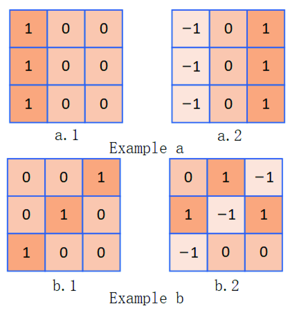
• DDC is proposed to extract the main gradient information from image through the difference operation on pixels.
• To balance the propertion of traditional convolution and DDC and further improve the overall performance, the two convolutions are weighted and optimized by a parameter. Experiments show that DDC could make up for the deficiency of traditional convolution and improve the feature extraction capability of convolution layer.

The following contents of this paper are as follows: Section 2 presents related work, including face anti-spoofing and convolution operations; Section 3 introduces the traditional convolutions, DDC, and the network structure used in face anti-spoofing detection; Section 4 introduces the datasets used in experiment, the test metrics, the parameter setting in the training process, and the experiment process; The experimental results are discussed in Section 5; Section 6 concludes the paper and imagines future work.

2. Related Work

2.1. Face Anti-Spoofing

In 2011, M$\ddot{\mathrm{aa}}\mathrm{tt}\ddot{\mathrm{a}}$ et al. [7] used LBP to encode image texture into enhanced feature histogram and support vector machine (SVM) [20] for classification. In 2013, Bharadwaj et al. [10] used motion amplification technology to amplify facial micromovements and LBP for feature extractions and classified through SVM. In 2016, Boulkenafet et al. [5] proposed a method based on the color texture analysis to detect whether the input image is a living face. In 2014, Yang et al. [11] firstly applied convolutional neural network (CNN) [12] to face anti-spoofing detection. In 2016, Li et al. [13] predicted the information of remote photoplethysmography (rPPG) by detecting pulses in images. Since there was no pulse information in photos and 3D masks, this method has significant effects on these two types of attacks but performs poorly on replay video attacks. In 2018, Liu et al. [14] designed DepthNet, which includes a CNN part and a recurrent convolutional neural network (RNN) [21] part. In the CNN part, the depth map representing facial depth information with 2D images is used as supervision information. After training, the network can predict the corresponding depth map of the image through the input RGB image. The RNN part can predict the information of rPPG through the depth map obtained from the CNN part. In 2020, Yu et al. [15] proposed central difference convolution (CDC), which achieved good results in the central difference convolution network (CDCN) based on DepthNet [14] optimized by neural architecture search (NAS) [22,23]. However, its results show that it still falls short on some attack types.

2.2. Convolution Operations

Convolutions are widely used in deep neural networks to extract features from images. In recent years, traditional convolution in networks has also been extended and modified. Yu et al. [24] proposed a new convolutional network module dedicated to dense prediction based on dilated convolution. Dai et al. [25] introduced deformable convolution into the network by adding additional offsets in order to increase the spatial sampling positions in the module. The local binary convolution proposed by Felix et al. [26] reduces the number of parameters compared to traditional convolution. Moreover, pixel-level differential convolution [27] has also been proposed for edge detection. The main focus of these convolution methods is not on the fine-grained representation of images and may not be suitable for face detection tasks. Based on the problems and shortcomings of the above methods, we further explore and propose directional difference convolution.

3. DDC and Combined Convolution

The traditional convolution is first analyzed and discussed. Then, a new convolution is introduced to make up for its deficiency. According to the advantages of the traditional convolution and the new convolution, they are combined together and balanced through a parameter. Moreover, the face anti-spoofing detection network based on combined convolution is given.

3.1. Traditional Convolution

In deep learning, the convolutional operation is commonly used to extract features to reduce the dimension of images. In traditional convolution, the domain value of given kernel size is dot multiplication and then accumulation between the weight matrix of the convolution kernel and the pixel value matrix in the same size, which is:

$$y_{tra}\left(p_0\right)=\sum _{p_n\in \Re }w\left(p_n\right)·x(p_0+p_n).$$

(1)

where $p_0$ represents the current image domain, ℜ represents the collection of elements in the current image domain, $p_n$ represents each ordered position in the image domain, $x(p_0+p_n)$ represents the value of $p_n$ in the domain of the current position $p_0$, and $w\left(p_n\right)$ is the weight value of the convolution kernel corresponding to the position $p_n$, which is shown in Figure 1, $p_n$ are $(-1,1)$, $(0,1)$, $(1,1)$, $(-1,0)$, $(0,0)$, $(1,0)$, $(-1,-1)$, $(0,-1)$, and $(1,-1)$. Since the traditional convolution mainly multiplies and accumulates the weight value of the convolution kernel and the pixel value in the image matrix of the corresponding area and then uses this summation to replace the value of the entire area, it is essentially extracting the intensity information of the image [24,26,27]. However, the traditional image filtering operator is equivalent to performing a difference operation on the pixel values in the image domain when performing operations with the image domain due to the fixed value in the operator. Therefore, traditional image filtering operators such as Sobel [17,19] can extract gradient features well, such as image edges in traditional machine vision. Therefore, due to the limitations of traditional convolution operator, there is a shortage of gradient information extraction.

3.2. Directional Difference Convolution

The pixel gradients mean image texture and may exist in any direction, which contributes much to image recognition. In order to extract more valuable information from the image, the gradient information contained in the image can be further extracted and mined. Traditional convolution updates the weight of the convolution kernel according to the gradient descent of the loss function during the operation, which may obtain part of gradient information from the image whose proportion is too little to be submerged with image noise. This paper proposes a new convolution method, which is defined as directional difference convolution. In the convolution operation, pixels in the image domain covered by the convolution kernel are replaced by pixel difference, as shown in (2) and Figure 2.

$$y_{ddc}\left(p_0\right)=\sum _{p_n\in \Re }w\left(p_n\right)·(x(p_0+p_{n+1})-x(p_0+p_n)).$$

(2)

where $(p_0+p_{n+1})$ is the next position of $(p_0+p_n)$. For example, in a domain of $3\times 3$, all positions are shown in Figure 1, where $(-1,1)$ is the first position in ℜ, and $(1,-1)$ is the last position in ℜ, and the position behind $(1,-1)$ is $(-1,1)$. The difference mode of DDC is shown in Figure 2. DDC can enhance gradient information through differential calculation in image domain. Figure 3 shows two typical examples of DDC. In Example a, a.1 is a field with size $3\times 3$, whose pixel values in the first column are all 1 and the other positions are all 0, representing a vertical line on the image. Through the directional differential operation, it can be seen in a.2 that the value of the first column in a.1 is transformed to the third column, while the value of first column becomes $-1$, indicating that the directional differential operation converts the original thin line into a thick line with a greater difference, which makes the original pixel gradient range more obvious and enables the network to learn more gradient features. Similarly, the oblique line in b.1 also becomes a wider line with greater pixel difference and more obvious gradient information as shown in b.2 after the directional differential operation. Summarily, the DDC would not only retain the image intensity information but also obtain more obvious gradient information. These gradient details could improve the learning ability of the whole network.

In Figure 4, the upper row images show its original size, while the lower row show their local magnification, respectively, which, from left to right, are the original image a of the input neural network, the feature map b after the traditional convolutional operation, the feature map c after the DDC operation, and the feature map d after the combined convolution operations. Take the eyelid part as an example: its gradient information is totally lost in the traditional convolution, while the corresponding DDC extracts this information well, which can be seen in image f and image g clearly.

3.3. Combined Convolution

The advantage of DDC in gradient information extraction can make up for the deficiency of traditional convolution in this aspect. Thus, DDC combined with traditional convolution would figure out more image details. This combination is named combined convolution, and a parameter $\theta$ is used to balance weights of traditional convolution and DDC, which is given as

$$y_{com}\left(p_0\right)=\theta ·y_{tra}\left(p_0\right)+(1-\theta )·y_{ddc}\left(p_0\right).$$

(3)

Simplify (3) to a more consistent formation to program design, which is

$$y_{com}\left(p_0\right)=(2·\theta -1)·(\sum _{p_n\in \Re }w\left(p_n\right)·x(p_0+p_n))+(1-\theta )·(\sum _{p_n\in \Re }w\left(p_n\right)·x(p_0+p_{n+1})).$$

(4)

where $p_n$ is the last position in ℜ and $p_{n+1}$ is the first position in ℜ. According to (3), the combined convolution only uses DDC at $\theta =0$, and the combined convolution only uses the traditional convolution at $\theta =1$. With the variation of $\theta$, the proportion of two convolutions in the combined convolution would also change accordingly, which changes the feature map generated by the combined convolution and therefore affects the output result of the network. In the examples shown in Figure 4, the combined convolution would not only retain the information extracted by traditional convolution but also include more gradient information extracted by DDC. The influence of $\theta$ on combined convolution is analyzed in the experiment.

3.4. The Network Structure

Liu et al. [14] reported the depth maps which represent 3D features of faces as labels to train the network and proposed the DepthNet. Then, Yu et al. [15] designed a central difference convolutional network (CDCN) based on the DepthNet, where the network consists of three block structures: Block1, Block2, and Block3, which contain three convolution layers and one maximum pooling layer, respectively. When the image of size $3\times 256\times 256$ is input into the network, Block1 structure would output the feature map of size $128\times 128\times 128$, Block2 structure would output the feature map of size $128\times 64\times 64$, and Block3 structure would output the feature map of size $128\times 32\times 32$. The three feature maps are dimensionally reduced into feature maps of size $128\times 32$ through corresponding sampling layers and spliced through splicing layers. Three convolution layers are used for dimensionality reduction layer by layer to extract high-dimensional features, and the depth map corresponding to the input image is estimated. The network structure of the original convolution kernel is replaced by the combined convolution as shown in Figure 5.

On the basis of CDCN, CDCN++ was designed by using neural network structure search technology in [15]. This structure also contains three blocks, and Block2 has four convolutional layers. When an image is input into the network, three blocks generate a feature map, respectively. Then the feature map is input into the attention layer and sampling layer and spliced through the splicing layer. Finally, two convolution layers are used to extract features and estimate the depth map corresponding to the input image. The structure of the original convolution kernel is replaced with combined convolution as shown in Figure 6, where the attention layer still uses traditional convolution.

4. Experiment

4.1. The Datasets

Due to the development of face anti-spoofing detection, researchers have reported various face anti-spoofing detection datasets. Four datasets, CASIA-MFSD [28], Replay-Attack [29], MSU-MFSD [30], and OULU-NPU [5], are used in the experiment. As shown in

Table 1. Details of each dataset used in the experiment.

Dataset	Object	Attack Type	Video
			Real	Fake	Total
CASIA-MFSD	50	Wrapped photo Cut photo Video	150	450	600
Replay-Attack	50	Printed photo Digital photo Video	200	1000	1200
MSU-MFSD	35	Printed photo HR video Mobile photo	110	330	440
Oulu-NPU	55	Printed photo Video	1980	3960	5940

, the CASIA-MFSD dataset contains 600 video clips of 50 objects, where each object has 12 video clips in four categories: Real living human face (Normal), Wrapped photo attack, Cut photo attack, and Video attack. The Replay-Attack dataset contains 1200 video clips of 50 objects, where each object can be classified into four categories: Real human face (Normal), Printed photo attack, Digital photo attack, and Playback video attack. The MSU-MFSD dataset contains 440 video clips of 35 obkects, where each object can be classified into four categories: Real living human face (Normal), Printed photo attack, HR video (high-definition playback video attack), and Mobile video (low-definition playback video attack). The OULU-NPU dataset contains 4950 video clips of 55 objects, which includes four evaluation rules Protocol 1, Protocol 2, Protocol 3, and Protocol 4., and Protocol 1 is mainly used to evaluate the generalization degree of face anti-spoofing detection method under unknown environmental conditions (such as illumination).

4.2. Test Metrics

Internal tests were carried out on CASIA-MFSD, Replay-Attack, and MSU-MFSD for proposed method in [4]. The main test metric is the area under the receiver operating characteristic (ROC) curve, known as AUC. The abscissa of ROC is the probability of judging a fake face as a real face, which is called the false positive rate (FPR), and the ordinate is the probability of judging a real face as a real face, which is called the true positive rate (TPR). The thresholds for a binary classification model may be set high or low, and each threshold setting results in different FPR and TPR. The (FPR, TPR) coordinates corresponding to each threshold of the model are drawn in the ROC space to become the ROC curve of the model. AUC measures the merits and demerits of classification methods, and the larger its value is, the more robust and correct the classification method is. Tests are performed on the OULU-NPU dataset using the test modality originally specified in the dataset, which specified four test modalities to evaluate the model’s generalization capability for different environments. The main test metric is the average classification error rate (ACER), which is the average of attack presentation classification error rate (APCER) and bona fide presentation classification error rate (BPCER) [31], as follows

$$ACER=\frac{\mathrm{APCER}+\mathrm{BPCER}}{2}.$$

(5)

APCER refers to the proportion of fake faces classified as real faces by face anti-spoofing methods, while BPCER represents the proportion of face anti-spoofing methods that classify real faces as fake faces. ROC, APCER, and BPCER need to count the number of correct and incorrect classifications according to different thresholds. When APCER is equal to BPCER on the validation dataset, the obtained threshold is used in the test dataset, and the ACER can be calculated by (5).

4.3. Experimental Process

According to the network training method in [15], the video in the dataset is decoded to extract frames to obtain images (denoted as Pic-A), and then the corresponding DepthMaps of size $32\times 32$ (denoted as DepthMap-Real) are generated through PRNet [32]. When training the network, DepthMap-Real are used as the DepthMap labels for living faces, and all zeros with a size of $32\times 32$ are used as the DepthMap labels for non-living faces (denoted as DepthMap-Fake). The network can make the output DepthMaps closer to the corresponding DepthMap labels of the input image by training; that is, if the living face image is input, the output DepthMap DepthMap-Out-Real is close to DepthMap-Real, and a DepthMap-Out-Fake DepthMap similar to DepthMap-Fake is output if a non-living face image is input. The characteristic patterns generated by the network are shown in Figure 7, in which a5 and b5 are the depth maps generated by the network. The depth map a5 corresponding to a1 contains more information than depth map b5 corresponding to b1. Then, according to (6), the sum of elements of the corresponding matrices of DepthMap-Real, DepthMap-Out-Real, and DepthMap-Fake can be calculated, respectively, $m_1$ norm $SU{M}_{DepthMap-Real}$, $SU{M}_{DepthMap-Out-Real}$, and $SU{M}_{DepthMap-Out-Fake}$.

$$SU{M}_{PIC}={\parallel PIC\parallel }_{m_1}=\sum _{i=1}^m\sum _{j=1}^n\left|pi{c}_{i,j}\right|.$$

(6)

where $PIC\in \{DepthMap-Real,DepthMap-Out-Real,DepthMap-Out-Fake\}$, $m,n$ represent the rows and columns of matrix $PIC$, respectively. According to (7), the specific value of $m1$ norm of the corresponding matrix DepthMap-Out to the $m1$ norm of the corresponding matrix DepthMap-Real is calculated, that is, the score of the network output DepthMap, where $PI{C}_{out}\in \{DepthMap-Out-Real,DepthMap-Out-Fake\}$, $PI{C}_{real}\in \{DepthMap-Real\}$. Finally, the corresponding ROC curve can be drawn through all the scores of the verification set, and the optimal threshold can be obtained to distinguish whether the network output is correct or not. According to the test criteria proposed in [31], the threshold of the test set needs a threshold obtained on the verification set.

$$score=\frac{SU{M}_{PI{C}_{out}}}{SU{M}_{PI{C}_{real}}}.$$

(7)

4.4. Experimental Methods and Hyperparameter Settings

The experimental methods are mainly divided into three aspects:

• Test the effect of various $\theta$ values;
• Cross-type testing among various types within the datasets;
• Cross-type testing between different types of datasets.

When testing the effect of various $\theta$ values, we use Protocol 1 of the OULU-NPU dataset, which defined the training set, validation set, and test set originally. We divided CASIA-MFSD, Replay-Attack, and MSU-MFSD datasets into four sub-datasets according to the types contained therein. For Cross-type testing among various types within the datasets, the type to be tested plus the real type is the test set, and the other two attack types plus the real type is the training set. When doing Cross-type testing between different types of datasets, the subtype to be tested plus the real types in that dataset are the test set, and all types of the other two datasets are the training set. The training equipment we used was Inspur AI server, whose operating system was CentOs 7.5 and the graphics card was NVIDIA TITAN V. The size of the convolution kernel used in the experiment is $3\times 3$, the initial learning rate ($lr$) is $2\times {10}^{-4}$, which is adjusted by the optimizer Adam, to $lr\times 0.5$. When testing the effect of $\theta$ with different values, the highest training round is set as 1200, and when testing the performance of combined convolution on different datasets, the highest training round is set as 600. Since the convergence rates in various tests are different, we set different hyperparameters for the three tests, as shown in

Table 2. Hyperparameters used in the experiment.

Hyperparameter	Test the Effect of Various $\mathit{\theta }$ Values	Intra Test	Inter Test
gpu number	3	3	3
initial learning rate	0.0002	0.0002	0.0002
kernel size	$3\times 3$	$3\times 3$	$3\times 3$
$\theta$	$0,0.1,\dots ,1.0$	0.6	0.6
batch size	8	8	8
step size	300	200	200
gamma	0.5	0.5	0.5
epochs	1200	600	600

. Intra test in the Table 2 represents Cross-type testing among various types within the datasets and Inter test in the Table 2 means Cross-type testing between different types of datasets.

5. Experimental Results

5.1. The Effect of $\theta$

In this section, combined convolution is evaluated using Protocol 1 of the OULU-NPU dataset. During the experiment, the CDCN and CDCN++ structures proposed in [15] are used, where the convolution kernel was replaced by combined convolution, and the values of $\theta$ are $0,0.1,0.2,\dots ,1$. Figure 8 shows the data obtained from this test, and it can be seen in Figure 8a, $\theta =0$ means that only DDC is used in the network, and ACER is 5.42%, while $\theta =1$ means that only traditional convolution is used, and the ACER is 5.73%. The ACER achieved from DDC is smaller than that achieved from traditional convolution, indicating that DDC extracts more information than traditional convolution. Moreover, ACER = 4.27% is achieved from combined convolution at $\theta =0.5$, which is less than the ACER obtained from DDC or traditional convolution merely, indicating that the features extracted by traditional convolution and DDC are effectively fused in CDCN, and the gradient information extracted by DDC makes up for the deficiency of traditional convolution. Meanwhile, it can be seen from Figure 8b that ACER is 3.96% at $\theta =0$, ACER is 6.77% at $\theta =1$, and ACER is 2.81% at $\theta =0.6$, which is better than when using traditional convolution or DDC merely. This shows that the features extracted by traditional convolution and DDC are effectively fused, and the gradient information extracted by DDC makes up for the deficiency of traditional convolution. Summarily, with the variation of $\theta$, ACER achieved from different combinations of the two convolutions has little change on CDCN except at $\theta =0.1$ and at $\theta =0.3$ but is better than that achieved from traditional convolution alone. On CDCN++, the combined convolution also achieves better results except at $\theta =0.1$ and at $\theta =0.3$, but the range of change is larger than that on CDCN, which indicates that the combined convolution needs to combine the two convolutions with a fine $\theta$ value on CDCN++. We can conclude that the combination of DDC and traditional convolution can obtain better performance than traditional convolution in most combination modes from these two sets of data. DDC makes up for the deficiency of the traditional convolution in extracting effective information in the face anti-spoofing detection task, which made a great contribution to the characteristics of the network learning.

For the case of $\theta =0.1$ and $\theta =0.3$, we input the image into the convolution layer to obtain the corresponding combined convolution feature map, shown in Figure 9 and Figure 10, where a is the original image, b is the image obtained at $\theta =0.1$, c is the image obtained at $\theta =0.3$, and d is the image obtained when $\theta$ was set to the value of minimum ACER achieved from the network. As can be seen from the figures, at $\theta =0.1$ or $\theta =0.3$, the obtained images are fuzzy and contain more noise, indicating that the results of the two convolutions in these two combinations have a great influence on each other, and the network weight cannot be optimized in the direction of the optimal gradient. In Figure 9d and Figure 10d, the edges are clear, and each edge contour in the image can be clearly distinguished, indicating that the two convolutions function together to fully extract the gradient information and suppress the noise information of the original image in this combination. Thus, the weight of the network is optimized, and the feature extraction ability of the neural network is improved, where CDCN++ is used in subsequent experiments, and $\theta$ is 0.6.

5.2. Cross-Type Testing among Various Types within the Datasets

The cross-type testing mainly evaluates the adaptability of the face anti-spoofing detection method to different sub-types in the dataset. Specifically, it tests the adaptability of the face anti-spoofing detection method to attacks that have not been encountered in the dataset. According to the test method proposed in [4], internal tests are carried out on CASIA-MFSD, Replay-Attack and MSU-MFSD datasets. To test the sub-class Video of CASIA-MFSD dataset, three sub-classes, Normal, Cut photo, and Wrapped photo, are used for training and testing on the two sub-classes Normal and Video. As shown in

Table 3. AUC(%) of combined convolution crossing type tests within different datasets.

Method	CASIA-MFSD			Replay-Attack			MSU-MFSD			Overall
	Video	Cut Photo	Wrapped Photo	Video	Digital Photo	Printed Photo	Printed Photo	HR Video	Mobile Video
OC-$SV{M}_{RBF}$+BSIF [4]	70.74	60.73	95.90	84.03	88.14	73.66	64.81	87.44	74.69	78.68 ± 11.74
$SV{M}_{RBF}$+LBP [5]	91.94	91.70	84.47	99.08	98.17	87.28	47.68	99.50	97.61	88.55 ± 16.2
NN+LBP [6]	94.16	88.39	79.85	99.75	95.17	78.86	50.57	99.93	93.54	86.69 ± 16.25
DTN [3]	90.0	97.30	97.50	99.90	99.90	99.60	81.60	99.90	97.50	95.90 ± 6.2
Wu’s fusion [33]	90.69	98.96	97.91	99.99	99.98	99.72	−	−	−	−
SAPLC [34]	90.67	92.67	90.67	96.25	97.75	87.50	−	−	−	−
CDCN [15]	98.48	99.90	99.80	100.00	99.43	99.92	70.82	100.00	99.99	96.48 ± 9.64
CDCN++ [15]	98.07	99.90	99.60	99.98	99.89	99.98	72.29	100.00	99.98	96.63 ± 9.15
OURS	100.00	100.00	100.00	99.99	99.48	99.48	87.29	100.00	100.00	98.47 ± 3.96

, combined convolution achieves the best effect on CASIA-MFSD dataset, where AUC = 100% can be achieved in all three types of attack methods. The results obtained on the Replay-Attack dataset are slightly inferior to CDCN and CDCN++, but the difference is not significant. In the Printed photo sub-class of MSU-MFSD dataset, the result of AUC is 87.29%, which is higher than the results of 81.6% obtained from DTN [3] before, indicating that combined convolution can better deal with the types of attacks in this kind of attacks that have not been encountered before. The Mobile photo sub-class also exceeded the result achieved by CDCN (99.99%). In general, the mean AUC and standard deviation of combined convolution on the three datasets tested are 98.47% and 3.96, which beats the current relevant methods.

5.3. Cross-Type Testing between Different Types of Datasets

The cross-type testing between different types of datasets mainly tests the ability of face anti-spoofing detection method to judge the attack form which has not been encountered before. According to [4], when testing the Video sub-class of CASIA-MFSD dataset, training is required using Normal, Printed photo, and Digital photo sub-classes of the Replay-Attack dataset and Normal and Printed photo subsets of the MSU-MFSD dataset. Normal and Video sub-classes of CASIA-MFSD dataset are used for testing. This method reduces the internal influence of the dataset to a minimum. Thus, the obtained test data can better reflect the objectivity of face anti-spoofing detection. As shown in

Table 4. AUC (%) of combined convolution crossing type tests between different datasets.

Method	CASIA-MFSD			Replay-Attack			MSU-MFSD			Overall
	Video	Cut Photo	Wrapped Photo	Video	Digital Photo	Printed Photo	Printed Photo	HR Video	Mobile Video
OC-$SV{M}_{RBF}$+BSIF [4]	67.59	51.01	96.33	46.54	63.24	38.88	62.06	80.56	64.06	63.36 ± 17.46
$SV{M}_{RBF}$+LBP [5]	77.41	87.14	69.48	69.64	73.31	71.85	55.39	96.02	94.88	77.24 ± 13.24
NN+LBP [6]	71.80	70.26	67.55	36.93	75.43	69.45	26.10	96.84	85.31	66.63 ± 22.11
GMM+LBP [6]	65.41	85.00	50.15	60.78	61.46	55.32	59.35	91.18	86.43	68.34 ± 15.09
OC-$SV{M}_{RBF}$+LBP [6]	64.94	85.75	55.15	84.83	72.62	57.34	60.90	68.41	75.51	69.49 ± 11.15
AE+LBP [6]	77.72	80.30	52.92	79.67	54.92	52.71	55.67	87.94	92.18	70.45 ± 16.18
CDCN [15]	85.69	67.90	69.93	88.41	92.39	96.06	72.86	99.21	99.04	85.72 ± 11.78
CDCN++ [15]	82.77	68.82	70.28	91.58	90.61	97.40	72.21	99.05	99.86	85.84 ± 11.95
OURS	86.83	75.34	73.88	78.97	91.73	96.37	79.70	98.93	98.93	86.74 ± 8.64

, the AUC achieved from combined convolution in the Video sub-class of CASIA-MFSD dataset and in the Printed photo sub-class of MSU-MFSD dataset is 86.83% and 79.70%, respectively, which are superior to the current methods. The AUC achieved from combined convolution in Wrapped photo sub-class of CASIA-MFSD dataset, Digital photo sub-class, and Printed photo sub-class of Replay-Attack dataset ranks second place in the current correlation methods, and the AUC achieved from combined convolution in HR video sub-class and Mobile sub-class of MSU-MFSD dataset ranks third place in the current correlation methods, both ranking in the forefront. At the same time, the AUC achieved from all sub-classes in the CASIA-MFSD dataset and the printed photo sub-classes in the MSU-MFSD dataset have a certain improvement over CDCN and CDCN++. Summarily, the average value of AUC achieved from combined convolution is 86.74%, and the standard deviation is 8.64, ranking first, which fully proves that combined convolution extracts more feature information from images and improves the feature extraction capability of the convolution layer.

6. Conclusions

Traditional convolution mainly extracts intensity information but gradient information from the images. To make up its deficiency in feature extraction and improve the learning ability of neural network, directional difference convolution is proposed to extract the gradient information of the image, which is based on the correlation across pixels in the image domain. Because of the emphasis of traditional convolution and directional difference convolution, they are combined, and the proportions in convolution are optimized by a parameter, which is defined as combined convolution. Experiments on public datasets show that the proposed method is effective with better feature extraction. In future studies, it is necessary to improve the usability of directional difference convolution; thereby, balance parameters can be adjusted adaptively with the training process of neural network so as to adapt to a wider range of tasks. In addition, based on the advantages of DDC in image gradient feature extraction, more industrial scenes can be tested in the future, since there are more typical gradient information, such as workpiece boundaries.

References

1. Jiang, F.; Liu, P.; Zhou, X. A Review on Face Anti-spoofing. Acta Autom. Sin. 2021, 47, 1799–1821. [Google Scholar] [CrossRef]
2. Ministry of Public Security of the People’s Republic of China. Face Recognition Applications in Security Systems—Testing Methodologies for Anti-Spoofing, GA/T 1212-2014. 2014. Available online: https://kns.cnki.net/kcms/detail/detail.aspx?dbcode=SCHF&dbname=SCHF&filename=SCHF2016110569&uniplatform=NZKPT&v=EoByl325oT1PAAFBPwr0Ypcrw3SsIcVSzcUL2R2GKgY1PvNDB1i0Vj_UcV-IFs8y (accessed on 15 December 2021).
3. Liu, Y.; Stehouwer, J.; Jourabloo, A.; Liu, X. Deep Tree Learning for Zero-Shot Face Anti-Spoofing. In Proceedings of the 2019 IEEE/CVF Conference on Computer Vision and Pattern Recognition (CVPR), Long Beach, CA, USA, 15–20 June 2019; pp. 4675–4684. [Google Scholar] [CrossRef] [Green Version]
4. Arashloo, S.R.; Kittler, J. An anomaly detection approach to face spoofing detection: A new formulation and evaluation protocol. In Proceedings of the 2017 IEEE International Joint Conference on Biometrics (IJCB), Denver, CO, USA, 1–4 October 2017; pp. 80–89. [Google Scholar] [CrossRef]
5. Boulkenafet, Z.; Komulainen, J.; Li, L.; Feng, X.; Hadid, A. OULU-NPU: A Mobile Face Presentation Attack Database with Real-World Variations. In Proceedings of the 2017 12th IEEE International Conference on Automatic Face Gesture Recognition (FG 2017), Washington, DC, USA, 30 May–3 June 2017; pp. 612–618. [Google Scholar] [CrossRef] [Green Version]
6. Xiong, F.; AbdAlmageed, W. Unknown Presentation Attack Detection with Face RGB Images. In Proceedings of the 2018 IEEE 9th International Conference on Biometrics Theory, Applications and Systems (BTAS), Redondo Beach, CA, USA, 22–25 October 2018; pp. 1–9. [Google Scholar] [CrossRef]
7. Määttä, J.; Hadid, A.; Pietikäinen, M. Face spoofing detection from single images using micro-texture analysis. In Proceedings of the 2011 International Joint Conference on Biometrics (IJCB), Washington, DC, USA, 11–13 October 2011; pp. 1–7. [Google Scholar] [CrossRef]
8. de Freitas Pereira, T.; Anjos, A.; De Martino, J.M.; Marcel, S.b. LBP-TOP Based Countermeasure against Face Spoofing Attacks. In Computer Vision-ACCV 2012 Workshops; Park, J.I., Kim, J., Eds.; Springer: Berlin/Heidelberg, Germany, 2013; pp. 121–132. [Google Scholar]
9. Yang, J.; Lei, Z.; Liao, S.; Li, S.Z. Face liveness detection with component dependent descriptor. In Proceedings of the 2013 International Conference on Biometrics (ICB), Madrid, Spain, 4–7 June 2013; pp. 1–6. [Google Scholar] [CrossRef]
10. Bharadwaj, S.; Dhamecha, T.I.; Vatsa, M.; Singh, R. Computationally Efficient Face Spoofing Detection with Motion Magnification. In Proceedings of the 2013 IEEE Conference on Computer Vision and Pattern Recognition Workshops, Portland, OR, USA, 23–28 June 2013; pp. 105–110. [Google Scholar] [CrossRef]
11. Yang, J.; Lei, Z.; Li, S.Z. Learn Convolutional Neural Network for Face Anti-Spoofing. arXiv 2014, arXiv:1408.5601. [Google Scholar]
12. LeCun, Y.; Boser, B.; Denker, J.S.; Henderson, D.; Howard, R.E.; Hubbard, W.; Jackel, L.D. Backpropagation Applied to Handwritten Zip Code Recognition. Neural Comput. 1989, 1, 541–551. [Google Scholar] [CrossRef]
13. Li, X.; Komulainen, J.; Zhao, G.; Yuen, P.C.; Pietikäinen, M. Generalized face anti-spoofing by detecting pulse from face videos. In Proceedings of the 2016 23rd International Conference on Pattern Recognition (ICPR), Cancun, Mexico, 4–8 December 2016; pp. 4244–4249. [Google Scholar] [CrossRef] [Green Version]
14. Liu, Y.; Jourabloo, A.; Liu, X. Learning Deep Models for Face Anti-Spoofing: Binary or Auxiliary Supervision. In Proceedings of the 2018 IEEE/CVF Conference on Computer Vision and Pattern Recognition, Salt Lake City, UT, USA, 18–23 June 2018; pp. 389–398. [Google Scholar] [CrossRef] [Green Version]
15. Yu, Z.; Zhao, C.; Wang, Z.; Qin, Y.; Su, Z.; Li, X.; Zhou, F.; Zhao, G. Searching Central Difference Convolutional Networks for Face Anti-Spoofing. In Proceedings of the 2020 IEEE/CVF Conference on Computer Vision and Pattern Recognition (CVPR), Seattle, WA, USA, 13–19 June 2020; pp. 5294–5304. [Google Scholar] [CrossRef]
16. Farid, H.; Simoncelli, E.P. Optimally rotation-equivariant directional derivative kernels. In Computer Analysis of Images and Patterns; Sommer, G., Daniilidis, K., Pauli, J., Eds.; Springer: Berlin/Heidelberg, Germany, 1997; pp. 207–214. [Google Scholar]
17. Sobel, I.; Feldman, G. An Isotropic 3 × 3 Image Gradient Operator. In Presentation at Stanford A.I. Project 1968. 2015. Available online: https://www.semanticscholar.org/paper/An-Isotropic-3%C3%973-image-gradient-operator-Sobel-Feldman/1ab70add6ba3b85c2ab4f5f6dc1a448e57ebeb30 (accessed on 15 December 2021).
18. Wang, X.; Li, X. Generalized Confidence Intervals for Zero-Inflated Pareto Distribution. Mathematics 2021, 9, 3272. [Google Scholar] [CrossRef]
19. Tian, R.; Sun, G.; Liu, X.; Zheng, B. Sobel Edge Detection Based on Weighted Nuclear Norm Minimization Image Denoising. Electronics 2021, 10, 655. [Google Scholar] [CrossRef]
20. Vapnik, V.N. Statistical Learning Theory; Wiley-Interscience: New York, NY, USA, 1998. [Google Scholar]
21. Zaremba, W.; Sutskever, I.; Vinyals, O. Recurrent Neural Network Regularization. arXiv 2014, arXiv:1409.2329. [Google Scholar]
22. Liu, H.; Simonyan, K.; Yang, Y. DARTS: Differentiable Architecture Search. arXiv 2019, arXiv:1806.09055. [Google Scholar]
23. Xu, Y.; Xie, L.; Zhang, X.; Chen, X.; Qi, G.J.; Tian, Q.; Xiong, H. PC-DARTS: Partial Channel Connections for Memory-Efficient Architecture Search. arXiv 2019, arXiv:1907.05737. [Google Scholar]
24. Yu, F.; Koltun, V. Multi-Scale Context Aggregation by Dilated Convolutions. arXiv 2016, arXiv:1511.07122. [Google Scholar]
25. Dai, J.; Qi, H.; Xiong, Y.; Li, Y.; Zhang, G.; Hu, H.; Wei, Y. Deformable Convolutional Networks. arXiv 2017, arXiv:1703.06211. [Google Scholar]
26. Juefei-Xu, F.; Boddeti, V.N.; Savvides, M. Local Binary Convolutional Neural Networks. In Proceedings of the 2017 IEEE Conference on Computer Vision and Pattern Recognition (CVPR), Honolulu, HI, USA, 21–26 July 2017; pp. 4284–4293. [Google Scholar] [CrossRef] [Green Version]
27. Su, Z.; Liu, W.; Yu, Z.; Hu, D.; Liao, Q.; Tian, Q.; Pietikäinen, M.; Liu, L. Pixel difference networks for efficient edge detection. In Proceedings of the IEEE/CVF International Conference on Computer Vision, Montreal, QC, Canada, 11–17 October 2021; pp. 5117–5127. [Google Scholar]
28. Zhang, Z.; Yan, J.; Liu, S.; Lei, Z.; Yi, D.; Li, S.Z. A face antispoofing database with diverse attacks. In Proceedings of the 2012 5th IAPR International Conference on Biometrics (ICB), New Delhi, India, 29 March–1 April 2012; pp. 26–31. [Google Scholar] [CrossRef]
29. Chingovska, I.; Anjos, A.; Marcel, S. On the effectiveness of local binary patterns in face anti-spoofing. In Proceedings of the 2012 BIOSIG-Proceedings of the International Conference of Biometrics Special Interest Group (BIOSIG), Darmstadt, Germany, 15–17 September 2012; pp. 1–7. [Google Scholar]
30. Wen, D.; Han, H.; Jain, A. Face Spoof Detection With Image Distortion Analysis. IEEE Trans. Inf. Forensics Secur. 2015, 10. [Google Scholar] [CrossRef]
31. International Organization for Standardization. ISO/IEC JTC 1/SC 37 Biometrics: Information Technology Biometric Presentation Attack Detection Part 1: Framework. 2016. Available online: https://www.iso.org/obp/ui/iso (accessed on 15 December 2021).
32. Feng, Y.; Wu, F.; Shao, X.; Wang, Y.; Zhou, X. Joint 3D Face Reconstruction and Dense Alignment with Position Map Regression Network. In Computer Vision–ECCV 2018; Ferrari, V., Hebert, M., Sminchisescu, C., Weiss, Y., Eds.; Springer International Publishing: Cham, Swizterland, 2018; pp. 557–574. [Google Scholar]
33. Wu, X.; Hu, W. Attention-based hot block and saliency pixel convolutional neural network method for face anti-spoofing. Comput. Sci. 2021, 48, 9. [Google Scholar]
34. Sun, W.; Song, Y.; Chen, C.; Huang, J.; Kot, A.C. Face Spoofing Detection Based on Local Ternary Label Supervision in Fully Convolutional Networks. IEEE Trans. Inf. Forensics Secur. 2020, 15, 3181–3196. [Google Scholar] [CrossRef]
Figure 1. Example of position inside .
Mathematics 10 00365 g001
Figure 2. Illustration of directional difference operation. (a) Schematic of the original image field. (b) Schematic of directional difference operation.
Mathematics 10 00365 g002
Figure 3. Examples of directional differential operation. (Example a): (a.1) Image with a vertical line. (a.2) Image of (a.1) after directional difference operation. (Example b): (b.1) Image with an oblique line. (b.2) Image of (b.1) after directional difference operation.
Mathematics 10 00365 g003
Figure 4. Feature graphs generated by two convolutions and their combination, where, (ad) are images of original size, while (eh) are their amplifications, respectively, from left to right, and are images after traditional convolution, images after DDC and images after combined convolution, respectively.
Mathematics 10 00365 g004
Figure 5. CDCN structure diagram with combined convolution.
Mathematics 10 00365 g005
Figure 6. CDCN++ structure diagram with combined convolution.
Mathematics 10 00365 g006
Figure 7. Feature graphs generated by CDCN++ networks with combined convolution, from (left) to (right) are the original real face image, feature map from Block1, feature map from Block2, feature map from Block3, and depth map from the network, respectively. (upper row): living face; (lower row): non-living face.
Mathematics 10 00365 g007
Figure 8. The effect of θ on CDCN (a) and CDCN++ (b).
Mathematics 10 00365 g008
Figure 9. The feature map corresponding to different θ on CDCN.
Mathematics 10 00365 g009
Figure 10. The feature map corresponding to different θ on CDCN++.
Mathematics 10 00365 g010